| Issue |
A&A
Volume 691, November 2024
|
|
|---|---|---|
| Article Number | A88 | |
| Number of page(s) | 9 | |
| Section | Interstellar and circumstellar matter | |
| DOI | https://doi.org/10.1051/0004-6361/202347351 | |
| Published online | 30 October 2024 | |
First map of D2H+ emission revealing the true centre of a prestellar core: Further insights into deuterium chemistry
1
LERMA & UMR8112 du CNRS, Observatoire de Paris, PSL Research University, CNRS, Sorbonne Universités,
75014
Paris,
France
2
Max-Planck-Institut für Radioastronomie,
Auf dem Hügel 69,
53121
Bonn,
Germany
★ Corresponding author; This email address is being protected from spambots. You need JavaScript enabled to view it.
Received:
3
July
2023
Accepted:
13
September
2024
Abstract
Context. IRAS 16293E is a rare case of a prestellar core being subjected to the effects of at least one outflow.
Aims. We want to disentangle the actual structure of the core from the outflow impact and evaluate the evolutionary stage of the core.
Methods. Prestellar cores being cold and depleted, the best tracers of their central regions are the two isotopologues of the trihydrogen cation that are observable from the ground: ortho-H2D+ and para-D2H+. We used the Atacama Pathfinder EXperiment (APEX) telescope to map the para-D2H+ emission in IRAS 16293E and collected James Clerk Maxwell Telescope (JCMT) archival data of ortho-H2D+. We compared their emission to that of other tracers, including dust emission, and analysed their abundance with the help of a 1D radiative transfer tool. The ratio of the abundances of ortho-H2D+ to para-D2H+ can be used to estimate the stage of the chemical evolution of the core.
Results. We have obtained the first complete map of para-D2H+ emission in a prestellar core. We compare it to a map of ortho-H2D+ and show their partial anti-correlation. This reveals a strongly evolved core with a para-D2H+/ortho-H2D+ abundance ratio towards the centre for which we obtain a conservative lower limit from 3.9 (at 12 K) to 8.3 (at 8 K), while the high extinction of the core is indicative of a central temperature below 10 K. This ratio is higher than predicted by the known chemical models found in the literature. Para-D2H+ (and indirectly ortho-H2D+) is the only species that reveals the true centre of this core, while the emission of other molecular tracers and dust are biased by the temperature structure that results from the impact of the outflow.
Conclusions. This study is an invitation to reconsider the analysis of previous observations of this source and possibly questions the validity of the deuteration chemical models or of the reaction and inelastic collisional rate coefficients of the H+3 isotopologue family. This could impact the deuteration clock predictions for all sources.
Key words: astrochemistry / radiative transfer / ISM: abundances / ISM: molecules / ISM: structure / ISM: individual objects: IRAS 16293E
The affiliation of B. Parise corresponds to her affiliation when the project was initiated.
© The Authors 2024
 Open Access article, published by EDP Sciences, under the terms of the Creative Commons Attribution License (https://creativecommons.org/licenses/by/4.0), which permits unrestricted use, distribution, and reproduction in any medium, provided the original work is properly cited.
This article is published in open access under the Subscribe to Open model. This email address is being protected from spambots. You need JavaScript enabled to view it. to support open access publication.
1 Introduction
IRAS 16293E is a well-known prestellar core (PSC) at a distance of 141 pc (Dzib et al. 2018) that is under the influence of at least one outflow coming from the multiple protostar system IRAS 16293–2422 (e.g. Wootten & Loren 1987; Castets et al. 2001; Lis et al. 2002; Stark et al. 2004). A second outflow, visible in the Spitzer InfraRed Array Camera (IRAC) data and coming from the young stellar object (YSO) WLY 2-69, was also reported by Pagani et al. (2015a). This outflow points towards the south of the PSC, close to the HE2 position (Castets et al. 2001), but whether this represents a fortuitous alignment or reveals an actual impact has not yet been established. IRAS 16293–2422 has attracted considerable attention as well, with the Sub-Millimeter Array (SMA) (Jørgensen et al. 2011) and Atacama Large Millimeter/submillimeter Array (ALMA) (programme PILS, Jørgensen et al. 2016, and follow-up papers), and the first (and still unique) detections of para-H2D+ and ortho-D2H+ in absorption in front of the Class 0 objects (Bruenken et al. 2014; Harju et al. 2017). IRAS 16293E has also gained new attention with the advent of ALMA observations combined with the Caltech Submillimeter Observatory (CSO) maps (Lis et al. 2016) after the detection of ND3 (Roueff et al. 2005), which confirm that most deuterated species such as N2D+ or DCO+ peak at the outflow–PSC interface, with the exception of ND2H and ND3, the emission of which peak about 10″ east of the DCO+ emission peak. In a preliminary study we showed that Herschel continuum observations of the source with the Photodetector Array Camera and Spectrometer (PACS) and Spectral and Photometric Imaging Receiver (SPIRE) instruments reveal the temperature gradient induced by the outflow, while ortho-H2D+ emission traces the cold part of the core, away from the working surface, and approximately coincidental with the core seen in absorption in Spitzer/IRAC mid-infrared images (Pagani et al. 2015a). The recent study by Kahle et al. (2023) of a large set of observations performed with the Atacama Pathfinder Experiment (APEX) telescope towards both the YSOs and the PSC improves the census of molecular abundances and better differentiates the various parts of this complex region, which confirms our understanding of its structure.
It has been shown that the deuterium chemistry evolves in a rather monotonic way during the PSC formation phase, and measuring the abundance of deuterated species could help to measure the time the cloud took to contract to the PSC core under scrutiny (Flower et al. 2006; Pagani et al. 2009; Pagani et al. 2013). Though it is easier to measure the deuteration of species such as NH3, HCO+, or N2H+, it has been advocated that measuring directly the abundance of the deuteration vector, namely the ![Mathematical equation: $\[\mathrm{H}_3^{+}\]$](/articles/aa/full_html/2024/11/aa47351-23/aa47351-23-eq2.png) isotopologues, would be a more precise way to characterize the evolution of the deuteration (Parise et al. 2011a,b; Harju et al. 2017). However, single point measurements are often ambiguous, provide only line-of-sight averaged values, often decreasing the contrast between species. Only maps of the species allow us to fully understand the physics and chemistry of the PSCs.
isotopologues, would be a more precise way to characterize the evolution of the deuteration (Parise et al. 2011a,b; Harju et al. 2017). However, single point measurements are often ambiguous, provide only line-of-sight averaged values, often decreasing the contrast between species. Only maps of the species allow us to fully understand the physics and chemistry of the PSCs.
In this paper, we present the first map of para-D2H+, towards the prestellar core IRAS 16293E, and compare it with archival data of ortho-H2D+, dust emission, and N2H+. Section 2 presents the observations. In Sect. 3, we analyse the emission of both deuterated isotopologues of ![Mathematical equation: $\[\mathrm{H}_3^{+}\]$](/articles/aa/full_html/2024/11/aa47351-23/aa47351-23-eq3.png) , and compare them to dust absorption and emission, and to N2H+ emission. We present a 1D modified Monte Carlo model in Sect. 4 to quantify the abundance of both isotopologues, and we discuss the various results in Sect. 5. Our conclusions are given in Sect. 6.
, and compare them to dust absorption and emission, and to N2H+ emission. We present a 1D modified Monte Carlo model in Sect. 4 to quantify the abundance of both isotopologues, and we discuss the various results in Sect. 5. Our conclusions are given in Sect. 6.
2 Observations
We observed para-D2H+ (![Mathematical equation: $\[\mathrm{J}_{K_a K_c}\]$](/articles/aa/full_html/2024/11/aa47351-23/aa47351-23-eq4.png) : 110−101) at 691.6604434 GHz (Jusko et al. 2017) with the Swedish-ESO PI Instrument for APEX (SEPIA660) receiver on the APEX 12 m telescope equipped with fast Fourier transform (FFT) backends, each with 65 536 channels of 61 kHz width. The observations were performed in several runs on ESO time (3 May 2021, 28–29 June 2021, project E-0105.C-0251A) and Max-Planck-Institute (MPI) time (24–26 March 2022, 1 April 2022, 4 April 2022, project M-0109.F-9501C-2022). We also included observations with the 7 pixel Carbon Heterodyne Array of the MPIfR (CHAMP+) camera taken on 7 September 2010 (one pointing, project M-085.F-0016-2010). The weather was exceptionally good (precipitable water vapour, PWV = 0.2–0.3 mm) during most of the SEPIA660 observations, and very good (PWV ≈ 0.5 mm) for the CHAMP+ observations. Apart from the seven positions observed with CHAMP+ and the two positions observed with SEPIA660 in May 2021, which were observed in position switching mode, all observations were done in the on-the-fly (OTF) mode to cover a 50″ × 50″ region (June 2021) extended to 50″ × 72″ in 2022 as the preliminary results indicated an unexpected emission to the south. The various reference positions are summarized in Table A.1. The total observing time is about 25 hours. The angular resolution is ~9″. The pointing was checked every hour, mainly on the nearby object RAFGL1922. The stability of the pointing is better than 3″. We used the Continuum and Line Analysis Single-dish Software (CLASS1) to subtract first-order baselines computed on the velocity range −24 to +31 km s−1, and smoothed the data (spatially, using XY_MAP) to 14″ and (spectrally) to 244 kHz (≈ 0.1 km s−1) to improve the sensitivity. The peak signal-to-noise ratio (S/N) is 7 in brightness temperature and 12 in integrated intensity (in the range 2.81–4.18 km s−1). The rms noise level in integrated intensity is 6.7 mK km s−1 (
: 110−101) at 691.6604434 GHz (Jusko et al. 2017) with the Swedish-ESO PI Instrument for APEX (SEPIA660) receiver on the APEX 12 m telescope equipped with fast Fourier transform (FFT) backends, each with 65 536 channels of 61 kHz width. The observations were performed in several runs on ESO time (3 May 2021, 28–29 June 2021, project E-0105.C-0251A) and Max-Planck-Institute (MPI) time (24–26 March 2022, 1 April 2022, 4 April 2022, project M-0109.F-9501C-2022). We also included observations with the 7 pixel Carbon Heterodyne Array of the MPIfR (CHAMP+) camera taken on 7 September 2010 (one pointing, project M-085.F-0016-2010). The weather was exceptionally good (precipitable water vapour, PWV = 0.2–0.3 mm) during most of the SEPIA660 observations, and very good (PWV ≈ 0.5 mm) for the CHAMP+ observations. Apart from the seven positions observed with CHAMP+ and the two positions observed with SEPIA660 in May 2021, which were observed in position switching mode, all observations were done in the on-the-fly (OTF) mode to cover a 50″ × 50″ region (June 2021) extended to 50″ × 72″ in 2022 as the preliminary results indicated an unexpected emission to the south. The various reference positions are summarized in Table A.1. The total observing time is about 25 hours. The angular resolution is ~9″. The pointing was checked every hour, mainly on the nearby object RAFGL1922. The stability of the pointing is better than 3″. We used the Continuum and Line Analysis Single-dish Software (CLASS1) to subtract first-order baselines computed on the velocity range −24 to +31 km s−1, and smoothed the data (spatially, using XY_MAP) to 14″ and (spectrally) to 244 kHz (≈ 0.1 km s−1) to improve the sensitivity. The peak signal-to-noise ratio (S/N) is 7 in brightness temperature and 12 in integrated intensity (in the range 2.81–4.18 km s−1). The rms noise level in integrated intensity is 6.7 mK km s−1 (![Mathematical equation: $\[\mathrm{T}_a^*\]$](/articles/aa/full_html/2024/11/aa47351-23/aa47351-23-eq5.png) scale) towards the centre of the map, and reaches ≈ 11 mK km s−1 at the edges. We assumed a main beam efficiency of ηMB ≈ 0.48 ± 0.048 for CHAMP+ observations2 and ηMB ≈ 0.46 ± 0.046 for SEPIA660 observations (Perez-Beaupuits, priv. comm.), which were applied to each set before merging them.
scale) towards the centre of the map, and reaches ≈ 11 mK km s−1 at the edges. We assumed a main beam efficiency of ηMB ≈ 0.48 ± 0.048 for CHAMP+ observations2 and ηMB ≈ 0.46 ± 0.046 for SEPIA660 observations (Perez-Beaupuits, priv. comm.), which were applied to each set before merging them.
We retrieved two sets of unpublished ortho-H2D+ (![Mathematical equation: $\[\mathrm{J}_{K_a K_c}\]$](/articles/aa/full_html/2024/11/aa47351-23/aa47351-23-eq6.png) : 110−111) observations at 372.421340 GHz (Jusko et al. 2017) from the James Clerk Maxwell 15 m Telescope (JCMT) archive3, from projects M07AU29 (2007) and M09AU01 (2009). They were obtained with the 16 pixel Heterodyne Array Receiver Program (HARP) receiver with the Auto Correlation Spectral Imaging System (ACSIS) backend (61 kHz sampling). The atmospheric opacity at 225 GHz ranged from 0.052 to 0.034 (M07) and from 0.04 to 0.02 (M09). The M07 data consists of a 600 s single pointing of 15 pixels (one corner detector was dead) towards the core centre. The M09 data (14 effective pixels) cover 232″×113″, one square jiggle map centred on the core (1200s integration) with an adjacent jiggle map to the east (300s integration). The M09 central map was presented in our conference poster (Pagani et al. 2015a). The original angular resolution of 13.2″ was smoothed to 14″ (after third-order baseline subtraction on a baseline extending from −21 to +28 km s−1, resampling, and smoothing with CLASS/XY_MAP). The frequency sampling was Hanning-smoothed to 122 kHz (≈0.1 km s−1). We assumed a main beam efficiency of ηMB ≈ 0.64. The peak S/N is 11 in brightness temperature and 19 in integrated intensity (in the range 2.92–4.28 km s−1). The average integrated intensity rms noise is 23 mK km s−1 for the central map, twice as high as for the eastern map of which we only used the edge to reach the emission limit of the core. The same observing run also provided us with N2H+ (J:4–3) observations at 372.6734633 GHz (Cazzoli et al. 2012), representative of many of the species observed towards the PSC (Lis et al. 2016; Kahle et al. 2023). The D2H+ and the H2D+ data sets are both resampled on a 7″ basis.
: 110−111) observations at 372.421340 GHz (Jusko et al. 2017) from the James Clerk Maxwell 15 m Telescope (JCMT) archive3, from projects M07AU29 (2007) and M09AU01 (2009). They were obtained with the 16 pixel Heterodyne Array Receiver Program (HARP) receiver with the Auto Correlation Spectral Imaging System (ACSIS) backend (61 kHz sampling). The atmospheric opacity at 225 GHz ranged from 0.052 to 0.034 (M07) and from 0.04 to 0.02 (M09). The M07 data consists of a 600 s single pointing of 15 pixels (one corner detector was dead) towards the core centre. The M09 data (14 effective pixels) cover 232″×113″, one square jiggle map centred on the core (1200s integration) with an adjacent jiggle map to the east (300s integration). The M09 central map was presented in our conference poster (Pagani et al. 2015a). The original angular resolution of 13.2″ was smoothed to 14″ (after third-order baseline subtraction on a baseline extending from −21 to +28 km s−1, resampling, and smoothing with CLASS/XY_MAP). The frequency sampling was Hanning-smoothed to 122 kHz (≈0.1 km s−1). We assumed a main beam efficiency of ηMB ≈ 0.64. The peak S/N is 11 in brightness temperature and 19 in integrated intensity (in the range 2.92–4.28 km s−1). The average integrated intensity rms noise is 23 mK km s−1 for the central map, twice as high as for the eastern map of which we only used the edge to reach the emission limit of the core. The same observing run also provided us with N2H+ (J:4–3) observations at 372.6734633 GHz (Cazzoli et al. 2012), representative of many of the species observed towards the PSC (Lis et al. 2016; Kahle et al. 2023). The D2H+ and the H2D+ data sets are both resampled on a 7″ basis.
We also used the JCMT Submillimeter Common-User Bolometer Array (SCUBA)-II 850 μm continuum observations obtained and published by Pattle et al. (2015). We refer to that paper for a detailed description of the observations. We retrieved Spitzer/IRAC data from the archive5. To the best of our knowledge, the PSC image from these observations has never been published, apart from our conference poster (Pagani et al. 2015a).
3 Analysis
Figure 1 shows the map of para-D2H+ (left panel). This is the first time that a map of para-D2H+ has been presented. The doubly deuterated ion follows precisely the IRAC-1 absorption image seen at 3.6 μm (central panel). Since D2H+ is expected to peak in the central coldest part of clouds, and since the total absence of stars at 3.6 μm reveals high extinction (typically AV ≥100 mag), these two maps trace the centre of the IRAS 16293E PSC, while the dust emission map peak (red cross), which is very sensitive to the temperature increase due to the outflow collision with the PSC edge, is displaced towards the impact point. Therefore, the dust emission map does not reveal the true cold centre of the PSC. In the right panel, the upper part of the IRAC-4 image of the PSC also seen in absorption is partially hidden (reduced contrast) by polycyclic aromatic hydrocarbon (PAH) emission in relation with another outflow mostly seen in the IRAC images. In the same panel, N2H+ (J:4–3) contours (in orange) also point towards the impact point, known as the DCO+ peak (e.g. Lis et al. 2016).
The left panel of Fig. 2 shows the ortho-H2D+ emission superimposed on the IRAC-1 image. It is again clearly shifted to the east compared to the dust emission peak and N2H+ (J:4–3) line emission peak (marked by the red cross) as we already reported in Pagani et al. (2015a) and has been confirmed by Kahle et al. (2023). It is remarkable that both dust and N2H+ emissions peak at the same place, probably revealing the exact position of the outflow impact on the PSC. On the other hand, as for para-D2H+ emission, dust absorption as seen by IRAC images is correlated with ortho-H2D+ emission. Dust in absorption is not sensitive to temperature effects, and this explains the decorrelation between dust absorption and emission. The dust absorption reveals the highest extinction part of the PSC, and as expected this coincides with the emission peak of ortho-H2D+ and para-D2H+. Another noticeable feature is the horseshoe shape of the ortho-H2D+ emission surrounding the PSC centre (the topmost grey-filled contour in Fig. 2, left side). This ortho-H2D+ horseshoe shape clearly surrounds the emission peak of para-D2H+, as shown in the right panel of Fig. 2. This indicates that the ortho-H2D+ emission is weaker towards the centre of the PSC. Since it is only the top contour of ortho-H2D+ emission that shows this feature, it means that only the inner part of the PSC shows a diminished emission, and therefore a diminished ortho-H2D+ abundance, compared to the outer layers. The intensity difference between the ortho-H2D+ peak emission at a right ascension offset of +7″ from the centre and the central position is 66 mK km s−1, with a respective statistical noise of 29 and 21 mK km s−1. The difference is 2.3σ, but if the ortho-H2D+ abundance had been constant, the emission would have increased towards the centre, as for para-D2H+, instead of decreasing. Therefore, the difference with respect to a situation where the abundance is constant is much higher than 2.3σ and statistically significant. In Sect. 4, we model the case of a constant ortho-H2D+ abundance to quantify the expected difference.
The pointed observations of ortho-H2D+ and para-D2H+ that were previously reported by Vastel et al. (2004) towards the position marked by a black cross in Figs. 1 and 2 are found to be inconsistent with our more sensitive mapping observations towards the same position. For para-D2H+, they reported a peak temperature of 0.34 K (±0.077 K ?)6 and a linewidth of 0.29 ±0.07 km s−1, to be compared with our 83 ±17 mK and a linewidth of 0.48 ±0.07 km s−1; for ortho-H2D+, they report a peak temperature of 1.31 K (±0.22 K ?)6 and a linewidth of 0.36 ±0.04 km s−1, to be compared with our 0.31 ±0.03 K and a linewidth of 0.61 ±0.04 km s−1. For a gas temperature in the range 16–25 K from earlier studies (Loinard et al. 2001; Castets et al. 2001; Lis et al. 2002; Stark et al. 2004; Lis et al. 2016) that applies to the DCO+ emission peak region, the thermal linewidth alone is expected to be between 0.38 and 0.48 km s−1 for para-D2H+ and between 0.43 and 0.54 km s−1 for ortho-H2D+, which are both inconsistent with the small linewidths reported by Vastel et al. (2004).
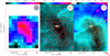 |
Fig. 1 Continuum and line emission images of IRAS 16293E. Left: colour map of para-D2H+ integrated intensity emission with white contours (colour scale and white contours from 0.01 to 0.07 by 0.01 K km s−1 plus a contour at 0.075 K km s−1; contour spacing of 0.01 K km s−1 = 1.5σ) Centre: IRAC-1 image at 3.6 μm. White contours trace para-D2H+ as in the left panel. The red contours trace the SCUBA-II 850 μm emission (20–160 by 20 [≈10σ] MJy sr−1). Right: IRAC-4 image at 8.0 μm. The white contours trace para-D2H+ as in the left panel. The orange contours trace the N2H+ (J:4–3) integrated intensity (0.3 to 2.3 by 0.4 [= 12σ] K km s−1). The yellow cross marks the centre of the D2H+ emission (αJ2000: 16h32m30.51s, δJ2000: −24°28′53.7″, see also Fig. 2). The red cross marks the peak position of the dust and N2H+ (J:4–3) emissions. The black cross (left panel) marks the position of the observation of D2H+ and H2D+ by Vastel et al. (2004). The yellow arrow traces the direction of the outflow from the IRAS 16293–2422 protostellar system and the red arrow the outflow from WLY 2-69. The grey and white disks represent the JCMT and APEX beams after smoothing to 14″. |
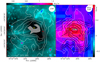 |
Fig. 2 Trihydrogen isotopologue maps with IRAC-1 image. Left: IRAC-1 image at 3.6 μm. The white contours trace ortho-H2D+. The filled grey contour marks the strongest emission (contours from 0.10–0.34 by 0.06 [=2.6σ] K km s−1). Right: para-D2H+ and ortho-H2D+ maps. Same map of para-D2H+ (black contours) as in Fig. 1, but superimposed on the ortho-H2D+ map (colour scale, plus white contours as in left panel). The yellow, black, and red crosses are as in Fig. 1. The D2H+, H2D+, and N2H+ spectra along the cut traced by the dashed line are displayed in Fig. 3. |
4 Radiative transfer modelling of para-D2H+ and ortho-H2D+
Modelling the abundance of both ![Mathematical equation: $\[\mathrm{H}_3^{+}\]$](/articles/aa/full_html/2024/11/aa47351-23/aa47351-23-eq7.png) isotopologues is needed to quantify our findings. The shape of the PSC is not symmetrical, but still relatively simple. There is however no easy way to derive its density and temperature structures, due to the complexity of its environment. Star counts or reddening measurements are impossible towards the centre of the core due to the lack of stars even in the sensitive Spitzer data (Fig. 1). The 8 μm continuum absorption measurements (Bacmann et al. 2000; Lefèvre et al. 2016) are hampered by the superposition of nebulosity emission from the IRAS 16293–2422A/B outflows and possibly some PAH emission. All emissions, whether dust or molecular, are strongly biased by the temperature gradient induced by the outflow impact on the PSC, and the density profile is also possibly perturbed on that side, away from a simple Plummer-like profile (Whitworth & Ward-Thompson 2001). To disentangle density, temperature, and abundances for molecules, or dust properties for continuum emission, a thorough analysis in 3D of the core must be performed. This is beyond the scope of the present paper and will be addressed in the future. Here we present a model combining three partially different one-dimensional (1D) spherical models.
isotopologues is needed to quantify our findings. The shape of the PSC is not symmetrical, but still relatively simple. There is however no easy way to derive its density and temperature structures, due to the complexity of its environment. Star counts or reddening measurements are impossible towards the centre of the core due to the lack of stars even in the sensitive Spitzer data (Fig. 1). The 8 μm continuum absorption measurements (Bacmann et al. 2000; Lefèvre et al. 2016) are hampered by the superposition of nebulosity emission from the IRAS 16293–2422A/B outflows and possibly some PAH emission. All emissions, whether dust or molecular, are strongly biased by the temperature gradient induced by the outflow impact on the PSC, and the density profile is also possibly perturbed on that side, away from a simple Plummer-like profile (Whitworth & Ward-Thompson 2001). To disentangle density, temperature, and abundances for molecules, or dust properties for continuum emission, a thorough analysis in 3D of the core must be performed. This is beyond the scope of the present paper and will be addressed in the future. Here we present a model combining three partially different one-dimensional (1D) spherical models.
The first step is to build 1D gas density and temperature structures of the PSC. The only tracer from the edge to the centre of the PSC is dust, especially in emission around 300 GHz, but its properties are not accurately known, and since the temperature and density profiles cannot be easily retrieved from the dust emission alone (Pagani et al. 2015b), we have constructed the core structure from the following considerations:
Except for the south-western extension, the emission of both para-D2H+ and ortho-H2D+ is relatively round and symmetrical. We consider that the bulk of the original core, before the outflow impacts its western side, is still present and close enough to a spherical object.
-
The eastern part of the core is unperturbed, and its H2 density can be described with a Plummer-like profile (Tafalla et al. 2002):
![Mathematical equation: $\[\mathrm{n}\left(\mathrm{H}_2\right)(\mathrm{r})=\frac{1.5 \times 10^6}{1+\left(\frac{\mathrm{r}}{3 \times 10^{16}}\right)^{2.5}} \mathrm{~cm}^{-3}.\]$](/articles/aa/full_html/2024/11/aa47351-23/aa47351-23-eq8.png) (1)
(1)The peak column density is 1.3 × 1023 cm−2, which is a visual extinction of AV ≈ 140 mag, compatible with the total absence of stars seen through the core, even in the Spitzer mid-infrared maps. It is also consistent with the dust emission at 850 μm towards the same spot (which is a weak constraint given the large uncertainty on the dust emissivity; Demyk et al. 2017a,b).
We also apply this profile to the west side. Using a different density profile would locally change the abundance profile of the ions, but would not impact the results for the central region of the core on first approximation.
In the centre of cold cores, temperatures are usually in the 8–12 K range (Caselli et al. 2008). We thus consider central temperatures of 8, 10, and 12 K and impose a temperature of 12 K in the external layers on the eastern side (the exact value has no impact in the 11–16 K range).
The N2H+ (J:4–3) emission peaks about 20″ west of the PSC centre in a place that is warmed by the outflow impact. Earlier studies proposed temperatures between 16 and 25 K (Loinard et al. 2001; Castets et al. 2001; Lis et al. 2002; Stark et al. 2004; Lis et al. 2016), and we display the results for the median value of 20 K, but also checked the 16 and 25 K cases.
The para-D2H+ spectra from −14″ to −28″ (and possibly −35″) in Fig. 3 are slightly stronger than their symmetrical ones eastward, and since the position of the peak of N2H+ emission is in the middle of this range, we set the temperature increase at −20″.
We divided the sphere into three parts. For each part, we ran a 1D spherical model, but we extracted the emission from the fraction of the sphere corresponding to that part only. We stitched the three extracted portions together and convolved the output to 14″. This is graphically explained in Appendix B. The spherical model is discretized into 20 layers of 1.14 × 1016 cm thickness. This corresponds to 5.4″ thickness per layer for a distance of 141 pc. The total size is 216″, which completely covers the core.
Though the warm part could be different in its density profile due to the possible compression from the outflow, if any (the outflow could be grazing the PSC and have only a limited compression effect), it is not possible to assess the actual profile at this stage until we have built a 3D model to explore that possibility. However, the warm part is far enough from the horseshoe-shaped central region and has no influence on the modelling of the cloud centre, as our tests have shown. Similarly, the impact of the temperature between 16 and 25 K was found to be negligible.
The modelled density, temperature, and isotopologue abundance profiles are displayed in Fig. 4. We adjusted the abundance, non-thermal linewidth, and radial velocity to fit the widths and strengths of the ortho-H2D+ and para-D2H+ lines (see synthetic spectra in Fig. 3). The linewidths show some inconsistencies, as revealed by Gaussian fits to the observed spectra (for more details, see Appendix C). This pseudo-1D modelling was performed with a 1D Monte Carlo code adapted from the Bernes (1979) radiative transfer programme. For the non-local thermodynamic equilibrium (non-LTE) modelling of the two ions, we used the inelastic collisional rate coefficients from Hugo et al. (2009). The abundances of both ions relative to H2 are displayed in the central panel of Fig. 4, while their ratio is displayed in the bottom panel.
The modelled lines are displayed in Fig. 3, and the same fit is traced in terms of integrated intensity in Fig. 5, where the centre of the ortho-H2D+ horseshoe shape is clearly visible. In Fig. 5, the observed intensities (solid lines, with their individual error bars) are reproduced within 1σ by the model (dashed line, same colour). Because the density keeps increasing towards the centre, the ortho-H2D+ intensity drop needs a strong abundance decrease to explain the decorrelation between the two (unlike para-D2H+, the intensity of which keeps increasing). Since the para-D2H+ abundance is found to be almost constant in the centre of the cloud (between 1.15 and 1.7 × 10⁻¹⁰, see below), we tested the case of a constant abundance for ortho-H2D+. The predicted intensity is shown in Fig. 5 with a dashed orange line. Towards the central position, the difference reaches 7σ and a uniform abundance of ortho-H2D+ is clearly excluded.
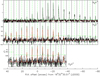 |
Fig. 3 N2H+ (J:4–3), ortho-H2D+ ( |
![Mathematical equation: $\[\mathrm{J}_{K_a K_c}\]$](/articles/aa/full_html/2024/11/aa47351-23/aa47351-23-eq9.png)
![Mathematical equation: $\[\mathrm{J}_{K_a K_c}\]$](/articles/aa/full_html/2024/11/aa47351-23/aa47351-23-eq10.png)
5 Discussion
The H2D+/D2H+ contrast reported in Sect. 3 is expected from the chemical evolution of the deuteration of the ![Mathematical equation: $\[\mathrm{H}_3^{+}\]$](/articles/aa/full_html/2024/11/aa47351-23/aa47351-23-eq11.png) ion (Roberts et al. 2003; Walmsley et al. 2004), which indicates that
ion (Roberts et al. 2003; Walmsley et al. 2004), which indicates that ![Mathematical equation: $\[\mathrm{H}_3^{+}\]$](/articles/aa/full_html/2024/11/aa47351-23/aa47351-23-eq12.png) can be converted to H2D+, itself converted to D2H+, and finally to
can be converted to H2D+, itself converted to D2H+, and finally to ![Mathematical equation: $\[\mathrm{D}_3^{+}\]$](/articles/aa/full_html/2024/11/aa47351-23/aa47351-23-eq13.png) , this last being potentially the most abundant ion at the end of the chemical evolution. The effect is greatest at the peak density because the higher the density, the faster the chemical reactions, other parameters being equal. This is the first time that we have directly witnessed the intermediate step of this transformation (
, this last being potentially the most abundant ion at the end of the chemical evolution. The effect is greatest at the peak density because the higher the density, the faster the chemical reactions, other parameters being equal. This is the first time that we have directly witnessed the intermediate step of this transformation (![Mathematical equation: $\[\mathrm{H}_3^{+}\]$](/articles/aa/full_html/2024/11/aa47351-23/aa47351-23-eq14.png) and
and ![Mathematical equation: $\[\mathrm{D}_3^{+}\]$](/articles/aa/full_html/2024/11/aa47351-23/aa47351-23-eq15.png) are not observable in dense clouds). This confirms that the original centre of the PSC is not coincident with the peak emission of species such as N2H+, N2D+, and DCO+, but 22″ apart, which differs from what is usually found in other objects (e.g. Tafalla et al. 2002; Pagani et al. 2007). This must result from the temperature enhancement produced by the molecular outflow hitting the PSC. This heating possibly explains the similar extent of H2D+ and D2H+ towards the working surface of the PSC, in the south-west direction. It may also explain the small secondary peak of para-D2H+ as a result of the temperature increase compensating the drop of abundance, although further work is needed to reach a firm conclusion.
are not observable in dense clouds). This confirms that the original centre of the PSC is not coincident with the peak emission of species such as N2H+, N2D+, and DCO+, but 22″ apart, which differs from what is usually found in other objects (e.g. Tafalla et al. 2002; Pagani et al. 2007). This must result from the temperature enhancement produced by the molecular outflow hitting the PSC. This heating possibly explains the similar extent of H2D+ and D2H+ towards the working surface of the PSC, in the south-west direction. It may also explain the small secondary peak of para-D2H+ as a result of the temperature increase compensating the drop of abundance, although further work is needed to reach a firm conclusion.
The column densities of both species derived from the modelling in Sect. 4 are nearly equal towards the centre, N(ortho-H2D+) peaks at 2.1 − 4.8 × 1013 cm−2 (at 12–8 K), and N(para-D2H+) at 0.94 − 4.2 × 1013 cm−2. The maximum para-D2H+/ortho-H2D+ column density ratio is ![Mathematical equation: $\[1.9_{-1.2}^{+2.1}\]$](/articles/aa/full_html/2024/11/aa47351-23/aa47351-23-eq16.png) , (at 10 K, ranging from 1.1 at 12K to 3.1 at 8 K)7. However, the derived abundance profiles yield a stronger contrast in the inner shells, as demonstrated in Fig. 5. For the two innermost shells (total radius of 10.8″), the abundance of ortho-H2D+ can be set to zero, while the line-of-sight emerging intensity computed by the model is still too high (but less than 1σ away from the observations). Since we asymptotically reach a difference of +0.8σ for the central position by decreasing the abundance by almost two orders of magnitude, we selected the abundance that provides exactly 1σ difference as the reference and computed the upper limit of this abundance by setting the error to 2σ. There is no lower limit since we cannot make the model weaker than the observations for this central spectrum because the large ortho-H2D+ abundance needed to reproduce the intensity of the line towards the walls of the horseshoe cavity is also sufficient to reproduce the intensity of the line for the two sightlines across the horseshoe hole, the same walls probably that are in front of and in back of the cavity, the observer having no privileged point of view (a situation similar to the case of L1506C, Pagani et al. 2010). In the centre of the cavity we find a very high para-D2H+/ortho-H2D+ abundance ratio of ~20. To check whether this ratio could be compatible with known models when taking into account the uncertainties of the line modelling, we computed a conservative lowest value of the uncertainty range of this ratio. We estimated an upper limit to the abundance of ortho-H2D+ at 2σ above the observations and found abundances of 1.8×10⁻¹¹ at 12 K, 3.05 × 10⁻¹¹ at 10 K, and 4.0 × 10⁻¹¹ at 8 K. We also computed a lower abundance for para-D2H+ by departing from the best fit abundance by −1σ (X[para-D2H+] = 6.95 × 10⁻¹¹, 1.3 × 10⁻¹⁰, and 3.3 × 10⁻¹⁰ at 12, 10, and 8 K respectively). The para-D2H+/ortho-H2D+ ratio lowest limit ranges from 3.9 to 8.3 (at 12–8 K).
, (at 10 K, ranging from 1.1 at 12K to 3.1 at 8 K)7. However, the derived abundance profiles yield a stronger contrast in the inner shells, as demonstrated in Fig. 5. For the two innermost shells (total radius of 10.8″), the abundance of ortho-H2D+ can be set to zero, while the line-of-sight emerging intensity computed by the model is still too high (but less than 1σ away from the observations). Since we asymptotically reach a difference of +0.8σ for the central position by decreasing the abundance by almost two orders of magnitude, we selected the abundance that provides exactly 1σ difference as the reference and computed the upper limit of this abundance by setting the error to 2σ. There is no lower limit since we cannot make the model weaker than the observations for this central spectrum because the large ortho-H2D+ abundance needed to reproduce the intensity of the line towards the walls of the horseshoe cavity is also sufficient to reproduce the intensity of the line for the two sightlines across the horseshoe hole, the same walls probably that are in front of and in back of the cavity, the observer having no privileged point of view (a situation similar to the case of L1506C, Pagani et al. 2010). In the centre of the cavity we find a very high para-D2H+/ortho-H2D+ abundance ratio of ~20. To check whether this ratio could be compatible with known models when taking into account the uncertainties of the line modelling, we computed a conservative lowest value of the uncertainty range of this ratio. We estimated an upper limit to the abundance of ortho-H2D+ at 2σ above the observations and found abundances of 1.8×10⁻¹¹ at 12 K, 3.05 × 10⁻¹¹ at 10 K, and 4.0 × 10⁻¹¹ at 8 K. We also computed a lower abundance for para-D2H+ by departing from the best fit abundance by −1σ (X[para-D2H+] = 6.95 × 10⁻¹¹, 1.3 × 10⁻¹⁰, and 3.3 × 10⁻¹⁰ at 12, 10, and 8 K respectively). The para-D2H+/ortho-H2D+ ratio lowest limit ranges from 3.9 to 8.3 (at 12–8 K).
This para-D2H+/ortho-H2D+ abundance ratio is high and is beyond all predictions made by various models, whether 0D (Pagani et al. 2009; Parise et al. 2011a,b), 1D (Pagani et al. 2013), or 3D (Bovino et al. 2019, 2021), which reach values of around 1–2 in the densest parts of the cores for a temperature of 10 K. Parise et al. (2011a,b) also found a ratio that was too high when analysing the H-MM1 prestellar core in the LDN 1688 star-forming region with a low temperature (7 K), but could reconcile the model and observations at 12 K. Here the 12 K value is possibly marginally consistent with the Bovino models if we interpolate by eye between their 10 and 15 K cases (Bovino et al. 2021, their Fig. B.2). However, clouds with Av ≥ 100 mag should be very cold in their centre, below 10 K following the models of Zucconi et al. (2001) and observations of Crapsi et al. (2007) and Pagani et al. (2007). These observations coupled to the present simple 1D modelling, if confirmed by a more accurate 3D modelling, either suggest that current chemical models are not yet close enough to reality to trace correctly the deuteration evolution of the tri-hydrogen ion in the cold medium or that the reaction rate coefficients or inelastic collisional rate coefficients of the ![Mathematical equation: $\[\mathrm{H}_3^{+}\]$](/articles/aa/full_html/2024/11/aa47351-23/aa47351-23-eq17.png) family with H2 and HD from Hugo et al. (2009), which were computed semi-classically, are not accurate enough and need to be improved. We found that increasing the collision rate coefficients of para-D2H+ with H2 by a factor of 6 or increasing the ortho-H2D+ + HD → para-D2H+ + para-H2 reaction rate coefficient by a factor of 3 would change the para-D2H+/ortho-H2D+ ratio by a factor of 2. Other similar changes can also be considered.
family with H2 and HD from Hugo et al. (2009), which were computed semi-classically, are not accurate enough and need to be improved. We found that increasing the collision rate coefficients of para-D2H+ with H2 by a factor of 6 or increasing the ortho-H2D+ + HD → para-D2H+ + para-H2 reaction rate coefficient by a factor of 3 would change the para-D2H+/ortho-H2D+ ratio by a factor of 2. Other similar changes can also be considered.
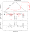 |
Fig. 4 Pseudo-1D model profiles of the core. Upper box: n(H2) Plummer-like profile in black. In red, temperature profile treated separately for the east (left) and the west (right) parts of the core, with three different minimum temperatures (10 K in plain line, 8 and 12 K in dashed lines). Middle box: ortho-H2D+ (black) and para-D2H+ (red) abundance profiles relative to H2 and computed separately for each side for the 10 K model, error bars are 1σ deviation from best model. Arrows mark upper limits. In particular, for ortho-H2D+ in the centre of the core, the dotted line represents the abundance to stay just below 1σ difference with the observations, and the upper error bar represents a difference of 2σ with the observations. Lower box: para-D2H+/ortho-H2D+ ratio for the 10 K model. Error bars are computed by taking the opposite error bars of both species when available, otherwise lower or upper limits are indicated by arrows. The long dashed and dash-dotted lines mark a ratio of 1 and 2, respectively, 2 being the upper limit of the models of Bovino et al. (2021) at 10 K. |
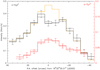 |
Fig. 5 Observed intensities along the horizontal cut (solid lines with error bars, corresponding to the spectra from Fig. 3) and corresponding model intensities (dashed lines). For ortho-H2D+ we present an additional model (orange dashed line) for which the abundance is kept constant across the core. Para-D2H+ observations and model (in red) have their own intensity axis (also in red) on the right side of the plot. |
6 Conclusions
We present in this article the first map of para-D2H+ in the interstellar medium, obtained with the APEX telescope towards the prestellar core IRAS 16293E. The main conclusions of this work are the following:
Maps of para-D2H+, and to a lesser degree of ortho-H2D+, reveal the position of the core centre before it was compressed and heated by at least one outflow coming from nearby YSOs. The new reference position for the core centre is αJ2000: 16h32m30.51s, δJ2000: −24°28′53.7″;
We derived peak column densities of ~1–3 × 1013 cm−2 for both ions (at 10 K).
We derived a conservative lower limit of the para-D2H+/ortho-H2D+ abundance ratio in the centre of the PSC in the range 3.9–8.3 at 12–8 K, while the core extinction (AV ≥ 100 mag) is indicative of a central temperature below 10 K. This ratio is higher than the values that published chemical models predict for temperatures below or around 10 K;
Temperature effects induced by the outflow impact at the hotspot make the line emission of most species bright. Therefore, an analysis limited to the hotspot could miss the real peak abundance of species, in particular ND3 and other deuterated species, the emission of which peaks away from the ortho-H2D+ and para-D2H+ abundance peaks.
To confirm the present model, a thorough modelling of the core to disentangle the density and temperature variations induced by the outflow impact needs to take into account all available information (line emissions with several transitions per species, dust emission, and absorption lower limit) in a 3D model, though the main difficulty of this model will be to constrain the line-of-sight distribution of all parameters.
The high para-D2H+/ortho-H2D+ ratio measured in IRAS 16293E could suggest, if confirmed, that the inelastic collisions or reaction rate coefficients of the ![Mathematical equation: $\[\mathrm{H}_3^{+}\]$](/articles/aa/full_html/2024/11/aa47351-23/aa47351-23-eq18.png) isotopologues need to be revised or that the chemical models need to be refined in order to improve our understanding of the deuteration process in starforming regions. This might have an impact on the chemical clock of deuteration used to study many star-forming regions.
isotopologues need to be revised or that the chemical models need to be refined in order to improve our understanding of the deuteration process in starforming regions. This might have an impact on the chemical clock of deuteration used to study many star-forming regions.
Acknowledgements
Based on observations with the Atacama Pathfinder Experiment (APEX) telescope. At the time of the first observations presented in this paper, APEX was a collaboration between the Max Planck Institute for Radio Astronomy, the European Southern Observatory, and the Onsala Space Observatory. This research has made use of NASA’s Astrophysics Data System Abstract Service. It has also made use of observations from Spitzer Space Telescope and from the NASA/IPAC Infrared Science Archive, which are operated by the Jet Propulsion Laboratory (JPL) and the California Institute of Technology under contract with NASA. This research makes a large use of the CDS (Strasbourg, France) services, especially Aladin (Bonnarel et al. 2000), Simbad and Vizier (Ochsenbein et al. 2000). We are indebted to C. de Breuck for the observations in the ESO time and to all the observers at APEX. We thank P.F. Goldsmith for useful comments and M. Tafalla for his helpful advices and editorial work.
Appendix A Reference positions for the APEX para-D2H+ observations
Different reference positions were used for the various projects with APEX towards IRAS 16293E. We list them in Table A.1
Reference positions for the APEX observations.
Appendix B Model building
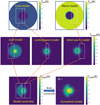 |
Fig. B.1 Steps to build an asymmetrical model from 1D spherical models. Based on a single density profile (eq. 1), we compute two models with different temperature profiles in the outer parts (either 12 or 20 K, top row, see Fig. 4). We apply two different abundance profiles (central row) for each ion for the east and west parts, the west part is computed for both temperature profiles. We extract the parts corresponding to each region of interest (sampled with a 1″ resolution) and we assemble them in a cube (RA, Dec, Frequency, bottom row left). Finally, we convolve the cube with a 14″ half-power beamwidth Gaussian beam to compare to the observations (bottom row right). We extract the spectra along the dash-dot line and compare them to the observations (see Fig. 3). |
The model is based on a single density profile (eq. 1) and we computed the emission on a 1″ step basis (model diameter of 216″) for various temperature and abundance profiles.
For positive offsets (east side) we used the pristine model and extracted the emission from the half sphere towards the east.
For offsets between 0 and −15″, we used the same model but on the west side with a different abundance profile except in the central shell which is forcibly common to both sides, being unresolved, (the centre being common to the east and west sides, we technically use only the west side and therefore the east stops at 5″, and the west goes from −15 to +5″)
For the external heated part, selected beyond −15″ from the centre, we used a 1D model with warm outer layers beyond a radius of 20″ in the western part.
For the ortho-H2D+ case shown in Fig. B.1, the strong dissymmetry is due to the fact that the emission is extended to the east and not as much to the west. The ortho-H2D+ abundance profiles (Fig. 4, central panel) reflect this difference by decreasing beyond −30″ on the western side, while it keeps increasing beyond +30″ on the eastern side. One should note that the warm layers beyond −20″ contribute to positions closer to the cloud centre, because being a 1D onion model, they are present on the line of sight of these closer positions in front and behind. The line of sight crosses a cold layer inserted between two hot layers. This could be justified by the outflow interacting with the surface of the PSC rather than ploughing its way to the centre, since the ortho-H2D+ and para-D2H+ lines do not seem to be kinematically perturbed in this warmer region. This problem will be examined in detail in a future work. The model is not representative of the emission towards the north or the south of the PSC.
Appendix C Linewidth and Gaussian fits of the D2H+ APEX and H2D+ JCMT spectra
The lines of both ions are optically thin (peak opacity of 0.6 and 0.7 for para-D2H+ and ortho-H2D+, resp.), and in first approximation consistent with a Gaussian shape. We have therefore adjusted a Gaussian to each of the spectra. These Gaussian fits are displayed in Fig. C.1. To adjust the Monte Carlo model, we modified the isotopologue abundance profile across the core to minimize the integrated intensity difference between the observations and the modelled line. Since the lines are optically thin, the exact shape of the line has little impact on its integrated intensity but of course, we take care that the linewidth be compatible with the observations. However, from the Gaussian fit, we found that the linewidth of the two isotopologues are not equal. At the edges, this is probably a noise limitation (e.g. the 21″ para-D2H+ spectrum), but in the centre, the para-D2H+ spectra at offsets 0, −7″, and −14″ are clearly larger than the ortho-H2D+ ones, for example for the 0 position:
δV(para-D2H+) = 0.658 ±0.074 km s−1
δV(ortho-H2D+) = 0.524 ±0.037 km s−1
H2D+ being lighter than D2H+, one would expect the former to display lines slightly wider than the latter for similar thermal turbulence or macroscopic movements. The reverse could indicate that the core inside the horseshoe, depleted in H2D+ (see Sect. 3), has a signature of collapse of its own traced by D2H+ alone, but we did not manage to reproduce this difference with our model. The volume is probably too small to dominate the linewidth formation without perturbing the H2D+ linewidth too. The other possibility is that this difference be mostly due to noise (1.8 σ difference) and we settled the model linewidth to be intermediate between these two values, making the D2H+ modelled line slightly stronger than the Gaussian fit but narrower, and conversely for H2D+.
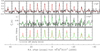 |
Fig. C.1 JCMT spectra of ortho-H2D+ JKK′:110−111 (top row, velocity axis from 1 to 6 km s−1), and APEX spectra of para-D2H+ JKK′:110−101 (middle row, velocity axis from 1 to 6 km s−1) across the cloud (the position of the cut is indicated in Fig. 2). Gaussian fits are overlaid in red and green, respectively. The same Gaussian fits with same colour code are reproduced in the bottom row, after normalization to the peak temperature for the +7″ spectrum, for a better comparison of the ratio variation and linewidth differences between the two isotopologues. |
References
- Bacmann, A., André, P., Puget, J.-L., et al. 2000, A&A, 361, 555 [Google Scholar]
- Bernes, C. 1979, A&A, 73, 67 [NASA ADS] [Google Scholar]
- Bonnarel, F., Fernique, P., Bienaymé, O., et al. 2000, A&AS, 143, 33 [NASA ADS] [CrossRef] [EDP Sciences] [Google Scholar]
- Bovino, S., Ferrada-Chamorro, S., Lupi, A., et al. 2019, ApJ, 887, 0 [Google Scholar]
- Bovino, S., Lupi, A., Giannetti, A., et al. 2021, A&A, 654, A34 [NASA ADS] [CrossRef] [EDP Sciences] [Google Scholar]
- Bruenken, S., Sipilä, O., Chambers, E. T., et al. 2014, Nature, 516, 219 [NASA ADS] [CrossRef] [Google Scholar]
- Caselli, P., Vastel, C., Ceccarelli, C., et al. 2008, A&A, 492, 703 [NASA ADS] [CrossRef] [EDP Sciences] [Google Scholar]
- Castets, A., Ceccarelli, C., Loinard, L., Caux, E., & Lefloch, B. 2001, A&A, 375, 40 [NASA ADS] [CrossRef] [EDP Sciences] [Google Scholar]
- Cazzoli, G., Cludi, L., Buffa, G., & Puzzarini, C. 2012, ApJS, 203, 11 [NASA ADS] [CrossRef] [Google Scholar]
- Crapsi, A., Caselli, P., Walmsley, M. C., & Tafalla, M. 2007, A&A, 470, 221 [NASA ADS] [CrossRef] [EDP Sciences] [Google Scholar]
- Demyk, K., Meny, C., Leroux, H., et al. 2017a, A&A, 606, A50 [NASA ADS] [CrossRef] [EDP Sciences] [Google Scholar]
- Demyk, K., Meny, C., Lu, X. H., et al. 2017b, A&A, 600, A123 [NASA ADS] [CrossRef] [EDP Sciences] [Google Scholar]
- Dzib, S. A., Ortiz-León, G. N., Hernández-Gómez, A., et al. 2018, A&A, 614, A20 [NASA ADS] [CrossRef] [EDP Sciences] [Google Scholar]
- Flower, D., Pineau Des Forêts, G., & Walmsley, C. M. 2006, A&A, 449, 621 [NASA ADS] [CrossRef] [EDP Sciences] [Google Scholar]
- Harju, J., Sipilä, O., Brünken, S., et al. 2017, ApJ, 840, 63 [NASA ADS] [CrossRef] [Google Scholar]
- Hugo, E., Asvany, O., & Schlemmer, S. 2009, JCP, 130, 164302 [Google Scholar]
- Jusko, P., Töpfer, M., Müller, H. S., et al. 2017, J. Mol. Spectrosc., 332, 33 [NASA ADS] [CrossRef] [Google Scholar]
- Jørgensen, J. K., Bourke, T. L., Nguyen Luong, Q., & Takakuwa, S. 2011, A&A, 534, 100 [Google Scholar]
- Jørgensen, J. K., van der Wiel, M., Coutens, A., et al. 2016, A&A, 595, A117 [NASA ADS] [CrossRef] [EDP Sciences] [Google Scholar]
- Kahle, K. A., Hernández-Gómez, A., Wyrowski, F., & Menten, K. M. 2023, A&A, 673, A143 [NASA ADS] [CrossRef] [EDP Sciences] [Google Scholar]
- Lefèvre, C., Pagani, L., Min, M., Poteet, C., & Whittet, D. C. B. 2016, A&A, 585, L4 [NASA ADS] [CrossRef] [EDP Sciences] [Google Scholar]
- Lis, D. C., Gerin, M., Phillips, T. G., & Motte, F. 2002, ApJ, 569, 322 [NASA ADS] [CrossRef] [Google Scholar]
- Lis, D. C., Wootten, H. A., Gerin, M., et al. 2016, ApJ, 827, 1 [NASA ADS] [CrossRef] [Google Scholar]
- Loinard, L., Castets, A., Ceccarelli, C., Caux, E., & Tielens, A. G. G. M. 2001, ApJ, 552, L163 [NASA ADS] [CrossRef] [Google Scholar]
- Ochsenbein, F. and Bauer, P. & Marcout, J. 2000, A&AS, 143, 23 [NASA ADS] [CrossRef] [EDP Sciences] [Google Scholar]
- Pagani, L., Bacmann, A., Cabrit, S., & Vastel, C. 2007, A&A, 467, 179 [NASA ADS] [CrossRef] [EDP Sciences] [Google Scholar]
- Pagani, L., Vastel, C., Hugo, E., et al. 2009, A&A, 494, 623 [NASA ADS] [CrossRef] [EDP Sciences] [Google Scholar]
- Pagani, L., Ristorcelli, I., Boudet, N., et al. 2010, A&A, 512, A3 [NASA ADS] [CrossRef] [EDP Sciences] [Google Scholar]
- Pagani, L., Lesaffre, P., Jorfi, M., et al. 2013, A&A, 551, 38 [Google Scholar]
- Pagani, L., Lefèvre, C., Belloche, A., et al. 2015a, EAS Publ. Ser., 75, 201 [CrossRef] [EDP Sciences] [Google Scholar]
- Pagani, L., Lefèvre, C., Juvela, M., Pelkonen, V. M., & Schuller, F. 2015b, A&A, 574, L5 [NASA ADS] [CrossRef] [EDP Sciences] [Google Scholar]
- Parise, B., Belloche, A., Du, F., Güsten, R., & Menten, K. M. 2011a, A&A, 526, A31 [NASA ADS] [CrossRef] [EDP Sciences] [Google Scholar]
- Parise, B., Belloche, A., Du, F., Güsten, R., & Menten, K. M. 2011b, A&A, 528, C2 [NASA ADS] [CrossRef] [EDP Sciences] [Google Scholar]
- Pattle, K., Ward-Thompson, D., Kirk, J. M., et al. 2015, MNRAS, 450, 1094 [NASA ADS] [CrossRef] [Google Scholar]
- Roberts, H., Herbst, E., & Millar, T. J. 2003, ApJ, 591, L41 [CrossRef] [Google Scholar]
- Roueff, E., Lis, D. C., van der Tak, F. F. S., Gerin, M., & Goldsmith, P. F. 2005, A&A, 438, 585 [NASA ADS] [CrossRef] [EDP Sciences] [Google Scholar]
- Stark, R., van der Tak, F. F. S., Sandell, G., et al. 2004, ApJ, 608, 341 [NASA ADS] [CrossRef] [Google Scholar]
- Tafalla, M., Myers, P. C., Caselli, P., Walmsley, C. M., & Comito, C. 2002, ApJ, 569, 815 [Google Scholar]
- Vastel, C., Phillips, T. G., & Yoshida, H. 2004, ApJ, 606, L127 [Google Scholar]
- Walmsley, C. M., Flower, D. R., & Pineau des Forêts, G. 2004, A&A, 418, 1035 [NASA ADS] [CrossRef] [EDP Sciences] [Google Scholar]
- Whitworth, A. P., & Ward-Thompson, D. 2001, ApJ, 547, 317 [Google Scholar]
- Wootten, A., & Loren, R. B. 1987, ApJ, 317, 220 [NASA ADS] [CrossRef] [Google Scholar]
- Zucconi, A., Walmsley, C. M., & Galli, D. 2001, A&A, 376, 650 [NASA ADS] [CrossRef] [EDP Sciences] [Google Scholar]
https://sha.ipac.caltech.edu/applications/Spitzer/SHA/, aorkeys: 3651840, 5756160, 18324736, and 47121664.
In their paper, no numerical value of the rms error is provided. This value is an educated guess from their Fig. 3.
The peak column densities are not coincidental.
All Tables
All Figures
|
Fig. 1 Continuum and line emission images of IRAS 16293E. Left: colour map of para-D2H+ integrated intensity emission with white contours (colour scale and white contours from 0.01 to 0.07 by 0.01 K km s−1 plus a contour at 0.075 K km s−1; contour spacing of 0.01 K km s−1 = 1.5σ) Centre: IRAC-1 image at 3.6 μm. White contours trace para-D2H+ as in the left panel. The red contours trace the SCUBA-II 850 μm emission (20–160 by 20 [≈10σ] MJy sr−1). Right: IRAC-4 image at 8.0 μm. The white contours trace para-D2H+ as in the left panel. The orange contours trace the N2H+ (J:4–3) integrated intensity (0.3 to 2.3 by 0.4 [= 12σ] K km s−1). The yellow cross marks the centre of the D2H+ emission (αJ2000: 16h32m30.51s, δJ2000: −24°28′53.7″, see also Fig. 2). The red cross marks the peak position of the dust and N2H+ (J:4–3) emissions. The black cross (left panel) marks the position of the observation of D2H+ and H2D+ by Vastel et al. (2004). The yellow arrow traces the direction of the outflow from the IRAS 16293–2422 protostellar system and the red arrow the outflow from WLY 2-69. The grey and white disks represent the JCMT and APEX beams after smoothing to 14″. |
| In the text | |
|
Fig. 2 Trihydrogen isotopologue maps with IRAC-1 image. Left: IRAC-1 image at 3.6 μm. The white contours trace ortho-H2D+. The filled grey contour marks the strongest emission (contours from 0.10–0.34 by 0.06 [=2.6σ] K km s−1). Right: para-D2H+ and ortho-H2D+ maps. Same map of para-D2H+ (black contours) as in Fig. 1, but superimposed on the ortho-H2D+ map (colour scale, plus white contours as in left panel). The yellow, black, and red crosses are as in Fig. 1. The D2H+, H2D+, and N2H+ spectra along the cut traced by the dashed line are displayed in Fig. 3. |
| In the text | |
|
Fig. 3 N2H+ (J:4–3), ortho-H2D+ ( |
| In the text | |
|
Fig. 4 Pseudo-1D model profiles of the core. Upper box: n(H2) Plummer-like profile in black. In red, temperature profile treated separately for the east (left) and the west (right) parts of the core, with three different minimum temperatures (10 K in plain line, 8 and 12 K in dashed lines). Middle box: ortho-H2D+ (black) and para-D2H+ (red) abundance profiles relative to H2 and computed separately for each side for the 10 K model, error bars are 1σ deviation from best model. Arrows mark upper limits. In particular, for ortho-H2D+ in the centre of the core, the dotted line represents the abundance to stay just below 1σ difference with the observations, and the upper error bar represents a difference of 2σ with the observations. Lower box: para-D2H+/ortho-H2D+ ratio for the 10 K model. Error bars are computed by taking the opposite error bars of both species when available, otherwise lower or upper limits are indicated by arrows. The long dashed and dash-dotted lines mark a ratio of 1 and 2, respectively, 2 being the upper limit of the models of Bovino et al. (2021) at 10 K. |
| In the text | |
|
Fig. 5 Observed intensities along the horizontal cut (solid lines with error bars, corresponding to the spectra from Fig. 3) and corresponding model intensities (dashed lines). For ortho-H2D+ we present an additional model (orange dashed line) for which the abundance is kept constant across the core. Para-D2H+ observations and model (in red) have their own intensity axis (also in red) on the right side of the plot. |
| In the text | |
|
Fig. B.1 Steps to build an asymmetrical model from 1D spherical models. Based on a single density profile (eq. 1), we compute two models with different temperature profiles in the outer parts (either 12 or 20 K, top row, see Fig. 4). We apply two different abundance profiles (central row) for each ion for the east and west parts, the west part is computed for both temperature profiles. We extract the parts corresponding to each region of interest (sampled with a 1″ resolution) and we assemble them in a cube (RA, Dec, Frequency, bottom row left). Finally, we convolve the cube with a 14″ half-power beamwidth Gaussian beam to compare to the observations (bottom row right). We extract the spectra along the dash-dot line and compare them to the observations (see Fig. 3). |
| In the text | |
|
Fig. C.1 JCMT spectra of ortho-H2D+ JKK′:110−111 (top row, velocity axis from 1 to 6 km s−1), and APEX spectra of para-D2H+ JKK′:110−101 (middle row, velocity axis from 1 to 6 km s−1) across the cloud (the position of the cut is indicated in Fig. 2). Gaussian fits are overlaid in red and green, respectively. The same Gaussian fits with same colour code are reproduced in the bottom row, after normalization to the peak temperature for the +7″ spectrum, for a better comparison of the ratio variation and linewidth differences between the two isotopologues. |
| In the text | |
Current usage metrics show cumulative count of Article Views (full-text article views including HTML views, PDF and ePub downloads, according to the available data) and Abstracts Views on Vision4Press platform.
Data correspond to usage on the plateform after 2015. The current usage metrics is available 48-96 hours after online publication and is updated daily on week days.
Initial download of the metrics may take a while.