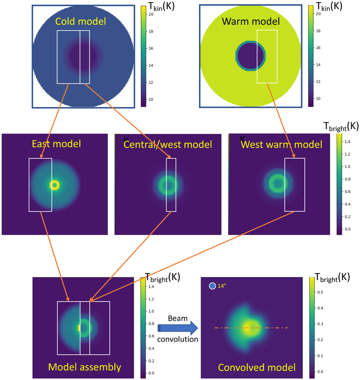
Fig. B.1
Download original image
Steps to build an asymmetrical model from 1D spherical models. Based on a single density profile (eq. 1), we compute two models with different temperature profiles in the outer parts (either 12 or 20 K, top row, see Fig. 4). We apply two different abundance profiles (central row) for each ion for the east and west parts, the west part is computed for both temperature profiles. We extract the parts corresponding to each region of interest (sampled with a 1″ resolution) and we assemble them in a cube (RA, Dec, Frequency, bottom row left). Finally, we convolve the cube with a 14″ half-power beamwidth Gaussian beam to compare to the observations (bottom row right). We extract the spectra along the dash-dot line and compare them to the observations (see Fig. 3).
Current usage metrics show cumulative count of Article Views (full-text article views including HTML views, PDF and ePub downloads, according to the available data) and Abstracts Views on Vision4Press platform.
Data correspond to usage on the plateform after 2015. The current usage metrics is available 48-96 hours after online publication and is updated daily on week days.
Initial download of the metrics may take a while.