| Issue |
A&A
Volume 690, October 2024
|
|
|---|---|---|
| Article Number | A42 | |
| Number of page(s) | 13 | |
| Section | Galactic structure, stellar clusters and populations | |
| DOI | https://doi.org/10.1051/0004-6361/202451595 | |
| Published online | 26 September 2024 | |
Optical observations of the Galactic supernova remnant HB9 and H II region G159.2+3.3
1
Purple Mountain Observatory, Chinese Academy of Sciences,
10 Yuanhua Road,
Nanjing
210023,
PR China
2
Department of Astronomy, Xiamen University,
422 Siming South Road,
Xiamen
361005,
PR China
3
School of Astronomy and Space Science, Nanjing University,
Nanjing,
Jiangsu
210093,
PR China
4
Key Laboratory of Modern Astronomy and Astrophysics, Nanjing University, Ministry of Education,
Nanjing
210093,
PR China
5
Key Laboratory of Radio Astronomy, Chinese Academy of Sciences,
Nanjing
210023,
PR China
Received:
22
July
2024
Accepted:
7
August
2024
Abstract
Context. We present multi-wavelength observations of the Galactic supernova remnant (SNR) HB9 and the H II region G159.2+3.3 apparently projected nearby, in order to study their properties and potential physical connections.
Aims. Confirming the physical connections between SNRs and H II regions is crucial to understanding their origin and interactions with the environment. Optical emission lines are powerful tools with which to measure the physical, chemical, and dynamical properties of the ionised gas, so could further help us to confirm such physical connections.
Methods. We present new optical narrow-band images of G159.2+3.3, as well as long-slit medium-resolution optical spectroscopy of both G159.2+3.3 and the SNR HB9 projected nearby. We compared these new data to archival multi-wavelength data to study the properties of the multi-phase interstellar medium in and around these two objects.
Results. HB9 is bright in γ-rays, but the γ-ray morphology is centrally filled and most of it is not clearly associated with the surrounding molecular clouds. There is a weak apparent connection of HB9 to the infrared bright enclosing shell of G159.2+3.3 in the γ-ray. The diffuse Balmer line has an almost identical morphology to the radio emission in G159.2+3.3, indicating they are both thermal in origin. Using medium-band high-resolution optical spectra from selected regions of the southeast (SE) shell of HB9 and G159.2+3.3, we found the radial velocity dispersion of HB9 along the slit to be significantly higher than the full width at half maximum of the lines. In contrast, these two values are both smaller and comparable to each other in G159.2+3.3. This indicates that the gas in HB9 may have additional global motion triggered by the SNR shock. The [N II] λ6583 Å/Hα line ratio of both objects can be interpreted with photo-ionisation by hot stars or low-velocity shocks, except for the post-shock region in the SE shell of HB9, where the elevated [N II]/Hα line ratio suggests a contribution from shock ionisation. The measured electron density from the [S II] 6716/6730 line ratio is significantly lower in the brighter G159.2+3.3 compared to the SE shell of HB9.
Conclusions. Our density estimate suggests that G159.2+3.3, although appearing brighter and more compact, is likely located at a much larger distance than HB9, so the two objects have no physical connections, unless the shock compressed gas in HB9 has a significantly lower filling factor.
Key words: ISM: bubbles / cosmic rays / H II regions / ISM: lines and bands / ISM: supernova remnants / ISM: individual objects: G159.2+3.3
Corresponding author; This email address is being protected from spambots. You need JavaScript enabled to view it.
© The Authors 2024
 Open Access article, published by EDP Sciences, under the terms of the Creative Commons Attribution License (https://creativecommons.org/licenses/by/4.0), which permits unrestricted use, distribution, and reproduction in any medium, provided the original work is properly cited.
This article is published in open access under the Subscribe to Open model. This email address is being protected from spambots. You need JavaScript enabled to view it. to support open access publication.
1 Introduction
Young stars form in giant molecular clouds, ionising the surrounding gas and forming H II regions, then become supernovae (SNe) after death and produce supernova remnants (SNRs). Multi-wavelength observations of H II regions and SNRs help us understand the star formation (SF) and feedback processes. More than 8000 H II regions have been discovered in the Milky Way (MW), most of them identified in the infrared (IR) due to the strong extinction in the optical band (e.g. Anderson et al. 2014). On the other hand, only about 300 Galactic SNRs have been identified, most commonly in the radio band (e.g. Green 2019, 2022). Only a small fraction of these SNRs have had their birth environment, and their physical connection to the surrounding H II regions, studied in detail (e.g. Chen et al. 2008; Zhou et al. 2018, 2023).
H II regions and SNRs are less commonly observed with large optical telescopes (e.g. van den Bergh et al. 1973; van den Bergh 1978), partially due to their distribution close to the Galactic plane and the resulting high extinction, and also because many of these sources have very large angular sizes. Optical observations, however, provide important information on the ionisation, heating, and dynamics of the ionised gas, which are key probes of the SF and feedback processes. Moreover, many of the H II regions and SNRs are sufficiently bright and large to be effectively observed with small telescopes using narrow-band imaging or spectroscopy (e.g. Parker et al. 1979; Fesen et al. 2024).
HB9 (G160.9+2.6) is a large Galactic SNR (angular size in Hα ≳ 2°), with a small (angular size in Hα ≲ 10′) H II region G159.2+3.3 apparently projected nearby. The Hα image of these two objects was first published by van den Bergh et al. (1973). HB9 appears as thin bright filaments in Hα, forming a semicircular shell that is bright in the southern half, with some more diffuse and fainter filaments forming an enclosed heart-like morphology in the northern side, while G159.2+3.3 appears brighter and more compact, and is located −2° north of the southern edge of HB9’s shell. D’Odorico & Sabbadin (1977) presented optical spectroscopy observations of the bright western edge of HB9, which reveal the average emission line ratios of Hα/[N II]≈ 1.33, [S II]λ6716/6730≈ 1.33, and Hα/[S II]≈ 1.72. Using the line ratio of the [S II] doublet, D’Odorico & Sabbadin (1977) obtained an electron density of ne = 690 cm–3, assuming a temperature of T ~ 104 K.
In the radio band, HB9 appears as multiple bright filaments forming a generally round shape (Leahy & Tian 2007; Gao et al. 2011). The average spectral index of the whole SNR is α ~ 0.5, and α is larger in the interior than on the bright shell, which can be explained by a lower interior magnetic field compared to that near the SNR shock. H I observations indicate a kinematic distance of 0.8 ± 0.4 kpc for the SNR (Leahy & Tian 2007), consistent with that derived from optical extinction (d = 0.54 kpc; Zhao et al. 2020). There is a radio pulsar, PSR B0458+46, located just ~23′ from the centre of HB9, but the latest radio absorption line observation indicates a lower limit of the distance to the pulsar (2.7 kpc), which is significantly greater than the distance to the SNR, suggesting it is a background source (Jing et al. 2023). The lack of a relation between the SNR and the pulsar also explains their significantly different ages (-6000 yr for the SNR, while the spindown age of the pulsar is -1.8 × 10⁶ yr; Leahy & Tian 2007). Compared to HB9, G159.2+3.3 is much more compact and even brighter in radio, with a morphology resembling the Hα image.
HB9 is also detected in X-rays and γ-rays. With ROSAT observations, Leahy & Aschenbach (1995) found a centrally brightened soft X-ray morphology possibly enclosed by the Hα and radio shells, showing no strong temperature variation across the SNR. The X-ray emission is generally brighter towards the southern Hα bright shells. These characteristics have been confirmed with deeper Suzaku observations, which further show recombining plasma inside the bright western shell (Sezer et al. 2019; however, see later analysis showing the non-necessity of the recombining plasma; Saito et al. 2020). Hard X-ray emission above 1.5 keV was detected towards HB9 (Yamauchi & Koyama 1993), but it can be described by a thermal plasma model (Sezer et al. 2019; Saito et al. 2020). Spatially resolved 1–300 GeV γ-ray emission was also detected with the Fermi data at a few positions towards HB9, with the strongest features apparently from the SNR interior and associated with the southern shell (Araya 2014; Sezer et al. 2019; Oka & Ishizaki 2022). G159.2+3.3 is not detected in X-ray or γ-ray in the literature.
We herein present new optical spectroscopic observations of HB9 and the neighbouring H II region G159.2+3.3, as well as new optical narrow-band images of the latter (Figs. 1, 2). The major goal is to confirm if there is a physical connection between HB9 and G159.2+3.3 or any other surrounding H II regions associated with the latter. The paper is organised as follows. In Sect. 2, we introduce our optical observations and data reductions. We further compare our new optical images to the multi-wavelength images, and discuss the scientific implications in Sect. 3. The main results and conclusions are summarised in Sect. 4. Errors are quoted at 1σ confidence level in the remaining part of the paper, unless specifically noted.
2 New optical observations and data reduction
2.1 Narrow-band images
We took narrow-band images of G159.2+3.3 with the McGraw-Hill 1.3m telescope at the Michigan-Dartmouth-MIT (MDM) observatory (Fig. 2). We used the 1024 × 1024 Templeton CCD mounted on the F7.5 focus, resulting in a field of view (FoV) of 8.49′ and a pixel size of 0.5″. The FoV almost covers the entire H II region bright in Hα. We used the OSU656nb3, OSU486.1/3, and OSU5007 filters in the 2.5-inch OSU interference filter set covering the Hα, Hβ, and [O III] λ5007Å lines. The full width at 50% peak transmission of these three filters is 40, 27, and 29 Å, respectively, with detailed information, including the transmission curve, available on the MDM website1. The data used in this paper were taken before the moonrise, with exposures of 5 × 600 s (on 2024.03.21), 5 × 600 s (on 2024.03.19), and 3 × 600 s (on 2024.03.18) for Hα, Hβ, and [OIII], respectively, depending on the weather and the calibration observations.
We used the Astropy affiliated package ccdproc (v1.3.0.post1; Craig et al. 2017) to reduce the MDM optical images. We used 40 columns of the overscan area to subtract the bias with the tool subtract_overscan. We then trimmed the overscan region using the tool trim_image. We used the instrument flats taken with a built-in continuous lamp to correct for vignetting. The instrument flats for different filters were processed using the same bias-subtraction and overscantrimming procedure, then re-normalised and stacked using the tool combine. Each science exposure was flat-corrected using the tool flat_correct, realigned, and combined together by calculating the median using combine to reject cosmic rays (CRs) and hot pixels. Since different science exposures taken on the same night are often quite close to each other on the sky, the prominent bright column of hot pixels is often not removed. We then combined the reduced images in different bands to produce the colour images in Figs. 2b–d.
2.2 Medium-band spectroscopy
We took medium-band optical spectra of a few selected regions from G159.2+3.3 and HB9 with the Boller & Chivens CCD Spectrograph (CCDS) mounted on the MDM 1.3m telescope. CCDS is a conventional optical grating spectrograph operating in -3200-9500 Å. There are six diffraction gratings available on CCDS. We chose the highest-resolution 1800 grooves/mm grating, which has a wavelength coverage of -330 Å on the 1200 × 800 CCD, a dispersion of 0.275 Å pixel–1 (0.75″ pixel–1 in the spatial direction), and a resolution of -0.3 Å at -4700 Å with a fixed 1″ slit on the 1.3 m telescope. We chose a centre wavelength of λcen ≈ 6603 Å, so the spectra cover approximately 6437-6756 Å. This band includes a few important emission lines, such as Hα λ6563 Å, [N II] λλ6548, 6583 Å, and [S II] λλ6716, 6730 Å.
For HB9, we placed the approximately 10'-long slit on the southeast (SE) outer shell, on a bright filament probably tracing the SNR’s forward shock (Fig. 1). This area was close to a γ-ray enhancement revealed by an earlier Fermi Large Area Telescope (Fermi-LAT) observation (Sezer et al. 2019), but with the latest Fermi data, it was identified as a point source and removed (Oka & Ishizaki 2022; Fig. 1a). We took two 3 × 1200 s exposures in two nights (March 29 and March 30 2024), both with the slit located on a bright star for an accurate target acquisition. The star is ~1' north of the Ha filament (Fig. 1d).
For G159.2+3.3, we placed the slit on an IR-bright star (RA, Dec = 04:58:30.3, +47:58:33), in order to better locate the slit and the spectra extracted along it (Fig. 2). The IR emission from this star was detected with the Midcourse Space Experiment (MSX; Deharveng et al. 2005). The slit length is slightly longer than the FoV of our narrow-band images taken with the MDM 1.3m and Templeton, and covers the eastern edge of the H II region, including the optical and radio faint but IR bright outer shell. This IR bright star is resolved into two comparably bright point sources with a separation of ≈3.5″ on the optical image, with some clearly extended [O III] emission detected surrounding them (Fig. 2c). We then placed the slit on these two point sources in different observations. One of the two observations (3 × 600 s on March 30 2024; the other has 3 × 1200 s on 27 March 2024) was taken during the last half hour of evening twilight, so the sky background may be slightly brighter (not quite significant, as is shown in Sect. 3.1).
We reduced the CCDS long-slit spectroscopy data with IRAF v2.17 (the Image Reduction and Analysis Facility) (Tody 1986, 1993). We first subtracted the bias with the overscan in the unilluminated columns of 1204–1231 with the IRAF task linebias. We then created the instrument flat with the built-in flat lamp. The CRs were initially cleaned with the IRAF task cosmicrays, and further removed by calculating the median value of three exposures. We chose the MDM 1.3m built-in Xenon arc lamp for wavelength calibration, as it has a few bright lines in the medium wavelength range of interest. We identified these lines using the IRAF task identify and reidentify, then calculated the transformation function using fitcoords and applied it to the raw spectral image using transform. We performed initial background subtraction using the IRAF task background. We next aligned different spectral images using the bright stars falling in the slit, then combined them together. We also made variance images as the measurement error. We applied extinction corrections for different airmasses using the IRAF task extinction. When performing aperture extraction, we first extracted a spectrum only from one bright star using apall. This spectrum was used for a careful background fitting and subtraction, as well as tracing the curvature of the 2D spectrum across the dispersion direction. We then extracted a few spectra in the spatial direction, each with an extent of 20 pixels (15"). Since most of these spectra were extracted from extended sources with no significant structures in the spatial direction, we adopted the same background and aperture trace models as for the bright star, which was located close to the centre of the slit. The extracted source spectra were then flux calibrated using the spectra of the standard star Feige 34, taken with exactly the same setting. We finally applied the heliocentric velocity correction by calculating it using the IRAF task rvcorrect, then used dopcor to actually shift the spectra. The reduced 2D spectra of HB9 and G159.2+3.3 are presented in Figs. 3 and 4, respectively.
We fitted the spectra extracted from individual regions using the curve fitting code LMFIT (Newville et al. 2024). We adopted a linear continuum plus five Gaussian models representing Hα λ6562.819 Å, [NII] λλ6548.05, 6583.45 Å, and [S II] λλ6716.440, 6730.816 Å, assuming that they have the same centroid velocity. The full width at half maximum (FWHM) of lines from different elements (H, N, and S) are not linked and could be slightly different. The fitting results, as well as some example spectra, are presented in the appendix (Tables A.1 and A.2; Fig. A.1).
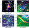 |
Fig. 1 Multi-wavelength images of the SNR HB9, the H II region G159.2+3.3, and the surrounding area. (a) False colour Fermi-LAT 1–300 GeV TS map centred on the SNR HB9. The white contours are the PMO 13.7 m 12CO (J=1–0) image from the MWISP–CO line survey, integrated in the velocity range of –13.0 – +6.5 km s–1. The γ-ray and CO enhancement in the upper part of the image is apparently associated with another SNR, G156.2+5.7. The 3.25° × 3.25° white box in the centre is the FoV of the images shown in panel b. (b) The red colour is the 4.85 GHz radio continuum image from the Green Bank 6-cm (GB6) survey (Gregory et al. 1996). The green colour is the DSS2 red-band image that covers the Hα line. The blue colour is the ROSAT/PSPC broad-band (0.1–2.4 keV) image obtained from the ROSAT All Sky Survey (RASS; Voges et al. 1999). The contours outline the Fermi-LAT image in panel a. The 0.93° × 0.93° white box in the lower left is the FoV of panel c, with the vertical bar overlaid on the bright SE filament marking the location of the MDM 1.3 m/CCDS slit. (c) Zoom-in of panel b, with the slit location plotted as a white bar, which is the same as the white bar in panel b. The 3.92° × 3.92° black box is the FoV of panel d. (d) Zoom-in PanSTARRS r-band image close to the centre of the slit. The double lines illustrate the width of the slit. |
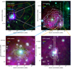 |
Fig. 2 Multi-wavelength images of the H II region G159.2+3.3. (a) NVSS 1.4 GHz (green and white contours) and WISE 12 µm (red)/22 µm (blue) images. The orange contours are the Fermi -LAT image presented in Fig. 1a. The 8.7′ × 8.7′ white box is the FoV of our MDM 1.3m optical images presented in panel b, while the vertical bar marks the approximate location of the CCDS slit. (b) Smoothed MDM 1.3m narrow-band images: Hα (red), [O III] λ5007 Å (green), Hβ (blue). The contours show the same NVSS image as in panel a. The two vertical lines are the locations of the slits used in the two CCDS spectroscopy observations, falling on two close (separated by ≈3.5″) bright stars, respectively. The smaller orange (1.52′× 1.52′) and bigger blue (2.71′ × 2.71′) boxes are the FoVs of panels c and d, which show two areas with possibly extended [OIII] emission (highlighted with white contours in these two panels). |
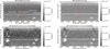 |
Fig. 3 2D spectra of the SE shell of HB9 extracted from the slit shown in Fig. 1. The left and right panels show the spectra taken on March 29 and March 30 2024, respectively. The y axis is the distance in arcmin from the bright star used for slit acquisition (appearing as a bright horizontal line), while the x axis is the wavelength in Å. The colour bar shows the intensity in units of ergs s–1cm–2 Å–1. Prominent emission lines are denoted. The vertical red lines in the upper panels show the wavelength range of the Hα and [N II] λ6583 Å lines, which is further zoomed in on in the lower panels. |
2.3 Archival multi-wavelength data used for comparison
In addition to the optical images described in Sect. 2.1, we also plot a few multi-wavelength images in Figs. 1 and 2 for comparison. We constructed the 1–300 GeV γ-ray image using more than 15 years (from August 04 2008 to March 28 2024) of the Fermi-LAT (Ajello et al. 2021) P8R3 data. We adopted the Galactic diffuse emission template, the isotropic diffuse spectral model and the Fourth Fermi-LAT source catalogue (4FGL; Abdollahi et al. 2020) to calculate the test statistics (TS) map with a pixel size of 0.05° in a 10° × 10° area around HB9.
We adapted the 12CO (J=1–0) data from the original one published in Zhou et al. (2023), which were obtained from the Milky Way Image Scroll Painting (MWISP)–CO line survey project2 using the Purple Mountain Observatory Delingha 13.7m millimetre wavelength telescope. The half-power beam width was ~51", and the data were meshed with a grid spacing of 30". The typical rms noise level of the integrated intensity in the 1.5 km s-1 velocity interval is ~0.25 K km s–1. We integrated in a broad velocity range of [-13.0, +6.5] km s-1 and present the full range 12CO (J=1–0) image as contours in Fig. 1a. We also obtained the ROSAT X-ray (0.1–2.4 keV) image, the Green Bank 6-cm (GB6) 4.85 GHz image, and the WISE IR (12, 22 µm) images from the SkyView Virtual Observatory (McGlynn et al. 1998), and plot them for comparison in Figs. 1 and 2.
3 Discussion
3.1 Comparison of multi-wavelength images
We compare the multi-wavelength morphology of HB9 and the surrounding area in Fig. 1a. This SNR is bright in γ-ray, but the γ-ray morphology is not clearly associated with the surrounding molecular clouds (Fig. 1a; Zhou et al. 2023). Instead, some other weaker γ-ray features in the surrounding area, such as the SNR G156.2+5.7 to the north (e.g. Gerardy & Fesen 2007), and a chain of γ-ray knots to the south, are apparently associated with some molecular gas features. The only molecular cloud apparently associated with the SNR HB9’s γ-ray emission is towards the SE shell, where the filament-like molecular cloud appears in a velocity range of [–5.5, –2.5] km s–1.
As is shown in Fig. 1b, the SNR HB9 is clearly detected in radio continuum at 4.85 GHz, appearing as an almost complete round shell with a typical diameter of ~20. The southern half of the shell has generally coherent optical counterparts, while the northern half does not. The SE part of the shell has two layers; both have specifically coherent optical/radio structures. The X-ray emission is relatively hard with little contribution at <0.4 keV, indicating strong extinction towards the SNR (NH ~ 4 × 1021 cm–2; Sezer et al. 2019). The bulk of the X-ray emission is enclosed within the inner SE shell, while there is no significant X-ray emission along the outer shell. Spectral analysis with the Suzaku data in Sezer et al. (2019) indicates that the western part of the X-ray emission is well described by a model that has collisional ionisation equilibrium (CIE) and recombining plasma components, while the eastern part is best reproduced by a CIE plus a non-equilibrium ionisation (NEI) model. The γ-ray morphology revealed by the latest Fermi-LAT data in this paper and Oka & Ishizaki (2022) is different from that constructed with the ~10 yr Fermi-LAT data in Sezer et al. (2019). The γ- ray brightest features are still the SNR interior approximately at the centre with no bright multi-wavelength counterparts, as well as the SE inner shell probably coherent with the inner optical and radio shells. However, unlike the images presented in Sezer et al. (2019), the SNR interior appears significantly brighter, and the source outside the SE outer shell has now been identified as a point source (4FGL J0506.6+4545) and removed. Another newly revealed interesting γ-ray feature is the weak enhancement slightly offset to the west of the H II region G159.2+3.3 (Figs. 1b, 2a). This feature, if real, may be physically connected to the dusty shell and the dense molecular cloud enclosing the H II region (see below). It may be a signature of the physical connection between these two objects; however, this needs to be further examined.
In Fig. 2, we present multi-wavelength images of the H II region G159.2+3.3 from both our new MDM narrow-band observations and the archival data. It is clear that the IR emission forms a shell enclosing the interior that is bright in both Balmer lines (Hα, Hβ) and the NVSS 1.4 GHz radio emission. A diffuse [O III] λ5007 Å line is almost non-detectable within the H II region, except for probably around two bright stars used for target acquisition and a point source at the centre (Figs. 2c,d). This multi-wavelength morphology is typical of H II regions (e.g. Anderson et al. 2011, 2014), which strongly indicates that both the Balmer lines and radio emission are thermal; the latter is produced in either a radio recombination line or the thermal Bremsstrahlung radiation (e.g. Terzian 1965; Anderson et al. 2011; Makai et al. 2017). On the other hand, forbidden lines and non-thermal radio emissions often elevated in shock are quite weak. The IR emission from the shell should be mainly produced by the dust heated by the ultraviolet (UV) photons from young stars, with the 12 µm emission dominated by polycyclic aromatic hydrocarbon molecules, while the 22 µm emission dominated by small dust grains (e.g. Anderson et al. 2014). We do not see any significant X-ray emission from G159.2+3.3, consistent with the above scenario that the emission of the H II region is dominated by the radiation-heated thermal emission with little contributions from shock heating.
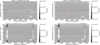 |
Fig. 4 Similar to Fig. 3, but for G159.2+3.3 extracted from the slits shown in Fig. 2. The slits used in the two nights (March 27 and March 30 2024) fall on two neighbouring stars ≈3.5" from each other. We do not see a significant difference between the spectra taken in these two nights, even though the spectra of March 30 2024 were taken during the evening twilight with a shorter exposure (Sect. 2.2). |
3.2 Radial velocity and gas dynamics
Measuring the radial velocity of a gas cloud provides a reliable method to estimate its distance, based on the MW kinematic model. Leahy & Tian (2007) found an H I 21-cm line emission enhancement spatially associated with only the boundary of HB9 in a local standard-of-rest (LSR) velocity range of VLSR = –3 to –9 km s–1, suggesting that the SNR is at a distance of d = 0.8 ± 0.4 kpc. In the MWISP CO survey, Zhou et al. (2023) identified only one broad CO line component towards HB9 at VLSR = -21.6 km s–1, which, however, shows no good spatial correlation with the remnant. Instead, they found better spatial correlation of the molecular gas with HB9 at VLSR ~ −2.5 km s−1. Furthermore, we also see some CO filaments in the velocity range of [−5.5, −2.5] km s−1 outside the SE shell of HB9, as is discussed in Sect. 3.1 and shown in Fig. la. The VLSR = −21.6 km s−1 component results in a distance of d = 2.1 ± 0.4 kpc, inconsistent with the estimate from optical extinction (Zhao et al. 2020). On the other hand, the VLSR ~ −2.5 km s−1 component indicates a distance of d = 0.5 ± 0.2 kpc, consistent with other estimates (Leahy & Tian 2007; Zhao et al. 2020), so could be associated with the SNR.
In the optical band, Lozinskaya (1981) found a mean radial velocity of VLSR = −18 ± 10 km s−1 of numerous filaments of either side of the expanding envelope of HB9, indicating a distance of d = 2 ± 0.8 kpc. No spectra and images are presented in Lozinskaya (1981), so it is difficult to justify where the velocities are measured. D’Odorico & Sabbadin (1977) presented measurements of the emission line ratios of HB9, but the spectral resolution is only Δλ ≈ 8 Å, insufficient to accurately measure the radial velocity.
With our medium-resolution MDM 1.3m/CCDS spectra, we measured the radial velocity at a few different locations of both HB9 (Table A.1) and G159.2+3.3 (Table A.2). The velocity profiles of the two objects along the slits (with the slit location marked in Figs. 1 and 2) are presented in Figs. 5d and 6d. The median radial velocity of the southern shell of HB9 is VLSR ≈ +1.9 km s−1, and spreads in a broad range of VLSR ~ [−30 to 50] km s−1 (see Tables A.l and A.2 for the measured values of individual regions). We can see that the largest velocity dispersion appears at a distance of approximately − 1′ to − 2′ (Fig. 5d), which is more clearly shown in the 2D spectra appearing as the distorted line shape (Fig. 3). In this area, the slit happens to be located on another bright star and penetrates some diffuse filaments (Fig. 1d). The large velocity dispersion of ΔVLSR ~ 80 km s−1 may indicate the heating or broadening of the gas by the SNR shock. In this case, the large range of measured VLSR is not inconsistent with any of the above radial velocity measurements.
The two observations of G159.2+3.3 show a clear systematic shift in the radial velocity of ~7.5 km s−1 (Fig. 6d). Since we reduced the data in an identical way and do not see a similar shift between the two observations of HB9 (Fig. 5d), we think the shift in G159.2+3.3 is likely real, caused by the relative motion of the gas falling into the two neighbouring slits (Fig. 2d). Compared to HB9, the velocity dispersion of G159.2+3.3 is significantly smaller, typically in the range of VLSR ~ [+2.5 − +20] km s−1, with a median value of approximately 11.7 km s−1. The VLSR of the two objects are thus overlapping each other. We therefore cannot rule out the possibility that HB9 and G159.2+3.3 are located at the same distance solely based on the radial velocity criterion.
The FWHMs of the lines in HB9 (median value of ~51.5 km s−1; Fig. 5e) are systematically higher than those in G159.2+3.3 (median value of ~36.3 km s−1; Fig. 6e). The additional broadening of the lines could be explained as the shock heating or broadening. While the FWHM of the lines in G159.2+3.3 is comparable to or slightly higher than the radial velocity dispersion along the slits (ΔVLSR ≲ 20 km s−1), the FWHM of HB9 is typically significantly lower than the velocity dispersion (ΔVLSR ~ 80 km s−1). This indicates that there is no significant global gas motion in the H II region G159.2+3.3, while such a global motion could be significant in an SNR-shocked region in HB9. We emphasise that our long slit is larger than the angular size of G159.2+3.3, so the measured velocity dispersion is largely representative of the whole H II region.
However, the slit just covers a small part of the SE shell of HB9, so the measured velocity dispersion is just a lower limit of the entire SNR, but should be representative of an SNR-shocked region.
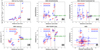 |
Fig. 5 Spatial distribution of parameters along the slit of HB9. Panels a-e are the Hα flux, the [N II]λ6583 Å/Hα flux ratio, the [S II]16716/6730 Å flux ratio, the centroid velocity, and the FWHM of the Hα line. Panel f is the [S II]16716/6730 Å-[N II]16583 Å/Hα line ratio diagram. The blue and red colours denote the data taken on the two nights, respectively. The distance in arcmin in panels a–e is measured from the bright target acquisition star, with north as negative and south as positive (Figs. 1, 3). In some panels, we also calculated the median value of the parameters (with significant outliers rejected) and denote them with a dotted green line. |
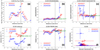 |
Fig. 6 Similar to Fig. 5 but for G159.2+3.3. Note that the slits used to extract the spectra in the two nights are slightly offset, located on two close but different acquisition stars (Fig. 6). |
3.3 Line ratio and physical properties of ionised gas
Physical parameters of the ionised gas could be measured with ratios of some emission lines (e.g. Haffner et al. 1999; Madsen et al. 2006; Osterbrock & Ferland 2006). For example, the electron density, ne, of the ionised gas could be measured with the ratio of two neighbouring density sensitive lines from the same ion, such as [S II] 6716/6730, [O II] 3729/3726, [Cl III] 5517/5537, [Ar IV] 4711/4740, C III] 1906/1909, and [N 1] 5202/5199, which is not affected by the reddening, the ionisation state, or the metal abundance (e.g. Copetti & Writzl 2002). The most commonly used ones are the strong [S II] and [O II] doublets, which are in general consistent with each other but which still show some small systematic offsets (e.g. Stanghellini & Kaler 1989; Copetti & Writzl 2002). The [S II] doublet is sensitive in a gas density range of ne ~ 101–5 cm−3, corresponding to a [S II] 6716/6730 line ratio of ~ 1.45−0.45 (Fig. 7). Using the [S II] doublet, D’Odorico & Sabbadin (1977) obtained an average 6716/6730 line ratio of 1.33 and an electron density of ne ≈ 690 cm−3 towards the western shell of HB9 (Sect. 1).
Our medium-band CCDS spectra simultaneously cover a few emission lines, including the [S II] doublet (Sect. 2.2; Figs. 3, 4, A.l). After rejecting the spectra from a few regions with poor signal-to-noise and/or background subtraction so nonphysical line ratios, we obtained a median [S II] 6716/6730 line ratio of ≈1.35 for the SE shell of HB9 (Fig. 5c; Table A.1) and ≈1.40 for G159.2+3.3 (Fig. 6c; Table A.2). The latter is quite close to the upper limit expected from the Te ~ 104 K gas (Fig. 7). In order to estimate ne, we plot the [S II] 6716/6730 line ratio as a function of both ne and Te in Fig. 8, using the PyNeb code3 (Luridiana et al. 2015). For ionised gas at Te > 103 K, at a line ratio of ℛ6716/6730 ≈ 1.35 for the SE shell of HB9, the electron density is ne ~ 102 cm−3 and insensitive to the temperature. This is roughly consistent with estimates from previous works in other parts of the SNR (D’Odorico & Sabbadin 1977). However, for G159.2+3.3, the [S II] 6716/6730 line ratio of ℛ6716/6730 ≈ 1.40 is quite close to the physical upper limit, and depends on both ne and Te. Assuming a typical ionised gas temperature of Te ~ 104 K, we can obtain ne ~ 50 cm−3. At any temperature, the derived ne should be significantly lower than that in HB9.
The lower ne of G159.2+3.3 than that of HB9, although estimated with large uncertainties, helps us to constrain the relative distance of the two objects. The flux density of an emission line (e.g. Hα; see the measured values in Tables A.1 and A.2) in a thermally emitting nebula can be described as
 (1)
(1)
where L is the luminosity of the object, d is the distance, θ is the angular size, V is the physical volume, and f is the volume filling factor. As is shown in both the images (Fig. 1b) and the Hα flux profiles (Figs. 5a, 6a), G159.2+3.3 has a significantly higher Hα flux density than HB9, but ne of G159.2+3.3 is indeed lower. For features with comparable angular sizes, G159.2+3.3 should have either a larger distance, d, or a significantly larger filling factor, f, than HB9. A larger distance to G159.2+3.3 (which should be about one order of magnitude larger to compensate for the lower ne, if all the measurements are accurate) seems to be consistent with its small angular size, although we cannot rule out the possibility of a small SF region being located at the same distance as the SNR (~0.9 – 1.8 pc, assuming the distance of HB9 is d ~ 0.5 – 1 kpc; Sect. 3.2). The same distance of G159.2+3.3 and HB9 is also not inconsistent with the radial velocity measurements (Sect. 3.2) and the γ-ray morphology (Sect. 3.1). On the other hand, if the SNR shock could significantly compress the ambient gas, as is expected, we may expect a significantly higher f in G159.2+3.3 than in the SE shell of HB9. This is an alternative explanation of the higher surface brightness but lower ne of G159.2+3.3, but requires a fine tuning of f. Without any further evidence of the physical interaction between them, we prefer the conclusion that the two objects are not physically connected to each other.
The forbidden-to-Balmer line ratio is often a good indicator of the excitation and ionisation mechanisms. Based on our CCDS spectra, we also present the [N II]/Hα line ratio of the two objects in Figs. 5b and 6b. As the [N II] 6548/6583 line ratio is almost a constant (≈ 1/3), we herein only discuss the flux ratio between the stronger [N II] λ6583 Å line and the Hα line. According to the ‘Baldwin, Phillips, & Terlevich’ (BPT) diagram (Baldwin et al. 1981), the median [N II] λ6583 Å/Hα line ratio of both the SE shell of HB9 (~0.48) and G159.2+3.3 (~0.27) could be classified as ‘H II regions’, indicating that the ionisa-tion sources are mainly hot stars, or in some cases also possibly low-velocity shocks in SNRs (e.g. Domček et al. 2023). However, at least in a few regions at a distance of ~ − 0.5′ − 0′ from the slit acquisition star (distance = 0) in HB9, we found some significantly elevated [N II] λ6583 Å/Hα line ratios up to ≳1, indicating additional ionisation sources. This sharp increase in the [N II] λ6583 Å/Hα line ratio is apparently associated with the post-shock area behind the bright SE shell (Fig. 1d), so the elevated line ratio could be direct evidence of shock ionisation or excitation of the ambient gas, if the nitrogen abundance is not significantly elevated.
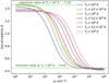 |
Fig. 7 Dependence of the [S II] 6716/6730 Å line ratio on the electron number density, ne. Different curves are the model predictions at different temperatures computed using PyNeb (Luridiana et al. 2015). The two dotted lines mark the approximate upper and lower physical limits on the [S II] 6716/6730 Å line ratio at Te ~ 104 K. |
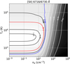 |
Fig. 8 Dependence of the [S II] 6716/6730 Å line ratio on the electron number density, ne, and temperature, Te. The grey-scale image and contours are the model predictions computed using PyNeb (Luridiana et al. 2015), with the corresponding line ratios denoted beside each contour. The blue (1.35) and red (1.40) contours are the median values measured in HB9 (Fig. 5c) and G159.2+3.3 (Fig. 6c), respectively. For high-density gas with ne ≳ 102 cm−3, the [S II] 6716/6730 Å line ratio is highly density dependant so a good density tracer. On the other hand, at ne ≲ 102 cm−3, [S II] 6716/6730 Å is less sensitive to density, but more affected by temperature. |
4 Summary
In this paper, we have presented optical observations of the Galactic SNR HB9 and the H II region G159.2+3.3 projected close to it. The new Hα, Hβ, and [O III] narrow-band images of G159.2+3.3 were taken with the MDM 1.3m telescope and the Templeton CCD. We also took medium-band medium-resolution spectra of a few selected regions in the SE shell of HB9 and G159.2+3.3 with the MDM 1.3m telescope and the CCDS spectrograph. Some prominent emission lines, such as Hα λ6563 Å, [N II] λλ6548, 6583 Å, and [S II] λλ6716, 6730 Å, are detected in many regions. We have measured the flux, centroid velocity, and ratios of the lines, and studied their spatial variation along the slits.
The main results of this paper are summarised below:
We compared the optical narrow-band images to some multi-wavelength images, including our reproduced Fermi-LAT image of more than 15 yr at 1–300 GeV, the 12CO (J=1−0) image from the MWISP–CO line survey, the ROSAT X-ray images, the WISE IR images, the radio images at 1.4 GHz from NVSS, and at 4.85 GHz from GB6. For HB9, we found that the Hα filaments are in general spatially correlated with the radio image, indicating that they are both produced by the SNR shock. The X-ray emission, however, is centrally filled and enclosed by the Hα and radio shells. This SNR is also bright in γ-rays, but the γ-ray morphology is not clearly associated with the surrounding molecular clouds, except probably for some molecular filaments in the velocity range of [−5.5, −2.5] km s−1 close to the SE shell.
Based on our new narrow-band images of the H II region G159.2+3.3, we found that the diffuse Balmer line emission has an almost identical morphology to the radio emission, both of them being enclosed by an IR bright shell, while the forbidden lines are quite weak. This multi-wavelength morphology is typical for Galactic H II regions, which indicates that the Balmer line and radio emissions in the interior are thermal in origin, while the IR bright shell consists of dust heated by the UV photons from young stars.
Based on our high-resolution spectra, we found that the radial velocity of the SE shell of HB9 sits in the range of VLSR ~ [−30−50] km s−1, consistent with previous measurements in other bands. This velocity dispersion over a small spatial scale indicates possible SNR shock heating of the gas. The velocity dispersion of G159.2+3.3 is significantly smaller, in the range of VLSR ~ [2.5–20] km s−1. The FWHM of the lines in G159.2+3.3 is slightly higher than the radial velocity dispersion, ΔVLSR, while the FWHM of HB9 is significantly smaller than ΔVLSR. This indicates additional global motion in HB9 caused by the SNR shock.
We further calculated the electron density, ne, from the [S II] 6716/6730 line ratio. We found a median ne of ~ 102 cm−3 for the SE shell of HB9 and a smaller median ne of ~50 cm−3 for the brighter G159.2+3.3. This could be explained by the distance of G159.2+3.3 indeed being larger than that of HB9 so that the two objects are not physically connected to each other, although we cannot rule out an alternative explanation that keeps the two objects physically connected but requires the filling factor of the shock compressed gas in the SNR to be significantly lower.
The [N II] λ6583 Å/Hα line ratio of both G159.2+3.3 and most areas of the SE shell of HB9 covered by our spectral analysis can be interpreted with photo-ionisation by hot stars or low-velocity shocks, such as in typical H II regions. However, in the post-shock region in the SE shell of HB9, we found an elevated [N II]/Hα line ratio, which indicates possible contributions from shock ionisation.
In conclusion, a physical connection between the SNR HB9 and the compact H II region G159.2+3.3 would require the filling factor of the ionised gas generated by shock compression in the SE shell of HB9 to be significantly lower than unity. We cannot rule out this possibility, so the physical connection between the two objects remains plausible but unclear based on the current data.
Acknowledgements
This research made use of IRAF, a general purpose software system for the reduction and analysis of astronomical data (Tody 1986, 1993); ccdproc, an Astropy affiliated package for image reduction (Craig et al. 2017); PyNeb, a lineage of tools dedicated to the analysis of emission lines (Luridiana et al. 2015). The authors acknowledge Eric Galayda at the MDM observatory for the help in setting up the MDM imaging and spectroscopy observations. J.T.L acknowledges the financial support from the National Science Foundation of China (NSFC) through the grants 12273111 and 12321003, and also the science research grants from the China Manned Space Project. Z.Q.X acknowledges the financial support from the Strategic Priority Research Programme of the Chinese Academy of Sciences No. XDB0550400 and the NSFC through the grant 12003069. Y.C acknowledges the financial support from the NSFC through the grants 12173018, 12121003, & 12393852. P.Z acknowledges the financial support from the NSFC through the grant 12273010. This research made use of the data from the Milky Way Imaging Scroll Painting (MWISP) project, which is a multi-line survey in 12CO/13CO/C18O along the northern galactic plane with PMO-13.7m telescope. We are grateful to all the members of the MWISP working group, particularly the staff members at PMO-13.7m telescope, for their long-term support. MWISP was sponsored by National Key R&D Programme of China with grants 2023YFA1608000 & 2017YFA0402701 and by CAS Key Research Programme of Frontier Sciences with grant QYZDJ-SSW-SLH047.
Appendix A Example spectra and spectral analysis results
The appendix shows two example spectra extracted from the SE shell of HB9 (Fig. A.1a) and the H II region G159.2+3.3 (Fig. A.1b), respectively. We also summarise spectral analysis results of different regions along the slits of the two objects in Tables A.1 and A.2. In the tables, we only list results of the regions with significant emission line features detected.
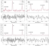 |
Fig. A.1 Example spectra (red solid lines) of (a, b) HB9 extracted on 2024.03.29 at the position of the acquisition star (d = 0, No.= 25; Fig. 1) and (c, d) G159.2+3.3 extracted on 2024.03.27 at d = −2.25′ from the acquisition star (No.= 15; Fig. 2). The grey solid curve is the best-fit to the spectra with Gaussian models plus a linear continuum. The lower panels show the spectral fit residuals defined as (model - data)/error. The slight difference in the residual continuum level in the upper and lower panels is caused by the imperfect local background modelling and subtraction, which however, does not affect the modelling of the emission lines. |
Spectral Analysis Results for HB9
Spectral Analysis Results for G159.2+3.3
References
- Abdollahi, S., Acero, F., Ackermann, M., et al. 2020, ApJS, 247, 33 [Google Scholar]
- Ajello, M., Atwood, W. B., Axelsson, M., et al. 2021, ApJS, 256, 12 [NASA ADS] [CrossRef] [Google Scholar]
- Anderson, L. D., Bania, T. M., Balser, D. S., & Rood, R. T. 2011, ApJS, 194, 32 [NASA ADS] [CrossRef] [Google Scholar]
- Anderson, L. D., Bania, T. M., Balser, D. S., et al. 2014, ApJS, 212, 1 [Google Scholar]
- Araya, M. 2014, MNRAS, 444, 860 [CrossRef] [Google Scholar]
- Baldwin, J. A., Phillips, M. M., & Terlevich, R. 1981, PASP, 93, 5 [Google Scholar]
- Chen, Y., Seward, F. D., Sun, M., & Li, J.-t. 2008, ApJ, 676, 1040 [NASA ADS] [CrossRef] [Google Scholar]
- Copetti, M. V. F., & Writzl, B. C. 2002, A&A, 382, 282 [NASA ADS] [CrossRef] [EDP Sciences] [Google Scholar]
- Craig, M., Crawford, S., Seifert, M., et al. 2017, https://doi.org/10.5281/zenodo.1069648 [Google Scholar]
- Deharveng, L., Zavagno, A., & Caplan, J. 2005, A&A, 433, 565 [NASA ADS] [CrossRef] [EDP Sciences] [Google Scholar]
- D’Odorico, S., & Sabbadin, F. 1977, A&AS, 28, 439 [Google Scholar]
- Domček, V., Hernández Santisteban, J. V., Chiotellis, A., et al. 2023, MNRAS, 526, 1112 [CrossRef] [Google Scholar]
- Fesen, R. A., Drechsler, M., Strottner, X., et al. 2024, arXiv e-prints [arXiv:2403.00317] [Google Scholar]
- Gao, X. Y., Han, J. L., Reich, W., et al. 2011, A&A, 529, A159 [NASA ADS] [CrossRef] [EDP Sciences] [Google Scholar]
- Gerardy, C. L., & Fesen, R. A. 2007, MNRAS, 376, 929 [NASA ADS] [CrossRef] [Google Scholar]
- Green, D. A. 2019, J. Astrophys. Astron., 40, 36 [Google Scholar]
- Green, D. A. 2022, Cavendish Laboratory, Cambridge, United Kingdom (available at http://www.mrao.cam.ac.uk/surveys/snrs/) [Google Scholar]
- Gregory, P. C., Scott, W. K., Douglas, K., & Condon, J. J. 1996, ApJS, 103, 427 [NASA ADS] [CrossRef] [Google Scholar]
- Haffner, L. M., Reynolds, R. J., & Tufte, S. L. 1999, ApJ, 523, 223 [CrossRef] [Google Scholar]
- Jing, W. C., Han, J. L., Hong, T., et al. 2023, MNRAS, 523, 4949 [NASA ADS] [CrossRef] [Google Scholar]
- Leahy, D. A., & Aschenbach, B. 1995, A&A, 293, 853 [NASA ADS] [Google Scholar]
- Leahy, D. A., & Tian, W. W. 2007, A&A, 461, 1013 [NASA ADS] [CrossRef] [EDP Sciences] [Google Scholar]
- Lozinskaya, T. A. 1981, Sov. Astron. Lett., 7, 17 [NASA ADS] [Google Scholar]
- Luridiana, V., Morisset, C., & Shaw, R. A. 2015, A&A, 573, A42 [NASA ADS] [CrossRef] [EDP Sciences] [Google Scholar]
- Madsen, G. J., Reynolds, R. J., & Haffner, L. M. 2006, ApJ, 652, 401 [CrossRef] [Google Scholar]
- Makai, Z., Anderson, L. D., Mascoop, J. L., & Johnstone, B. 2017, ApJ, 846, 64 [Google Scholar]
- McGlynn, T., Scollick, K., & White, N. 1998, IAU Symp., 179, 465 [NASA ADS] [Google Scholar]
- Newville, M., Otten, R., Nelson, A., et al. 2024, lmfit/lmfit-py: 1.3.1 [Google Scholar]
- Oka, T., & Ishizaki, W. 2022, PASJ, 74, 625 [CrossRef] [Google Scholar]
- Osterbrock, D. E., & Ferland, G. J. 2006, Astrophysics of Gaseous Nebulae and Active Galactic Nuclei (USA: University Science Books) [Google Scholar]
- Parker, R. A. R., Gull, T. R., & Kirshner, R. P. 1979, An Emission-line Survey of the Milky Way (NASA-Washington: Scientific and Technical Inform), 434 [Google Scholar]
- Saito, M., Yamauchi, S., Nobukawa, K. K., Bamba, A., & Pannuti, T. G. 2020, PASJ, 72, 65 [NASA ADS] [CrossRef] [Google Scholar]
- Sezer, A., Ergin, T., Yamazaki, R., Sano, H., & Fukui, Y. 2019, MNRAS, 489, 4300 [NASA ADS] [CrossRef] [Google Scholar]
- Stanghellini, L., & Kaler, J. B. 1989, ApJ, 343, 811 [NASA ADS] [CrossRef] [Google Scholar]
- Terzian, Y. 1965, ApJ, 142, 135 [NASA ADS] [CrossRef] [Google Scholar]
- Tody, D. 1986, SPIE Conf. Ser., 627, 733 [Google Scholar]
- Tody, D. 1993, ASP Conf. Ser., 52, 173 [NASA ADS] [Google Scholar]
- van den Bergh, S. 1978, ApJS, 38, 119 [NASA ADS] [CrossRef] [Google Scholar]
- van den Bergh, S., Marscher, A. P., & Terzian, Y. 1973, ApJS, 26, 19 [NASA ADS] [CrossRef] [Google Scholar]
- Voges, W., Aschenbach, B., Boller, T., et al. 1999, A&A, 349, 389 [NASA ADS] [Google Scholar]
- Yamauchi, S., & Koyama, K. 1993, PASJ, 45, 545 [NASA ADS] [Google Scholar]
- Zhao, H., Jiang, B., Li, J., et al. 2020, ApJ, 891, 137 [CrossRef] [Google Scholar]
- Zhou, P., Li, J.-T., Zhang, Z.-Y., et al. 2018, ApJ, 865, 6 [NASA ADS] [CrossRef] [Google Scholar]
- Zhou, X., Su, Y., Yang, J., et al. 2023, ApJS, 268, 61 [NASA ADS] [CrossRef] [Google Scholar]
All Tables
All Figures
|
Fig. 1 Multi-wavelength images of the SNR HB9, the H II region G159.2+3.3, and the surrounding area. (a) False colour Fermi-LAT 1–300 GeV TS map centred on the SNR HB9. The white contours are the PMO 13.7 m 12CO (J=1–0) image from the MWISP–CO line survey, integrated in the velocity range of –13.0 – +6.5 km s–1. The γ-ray and CO enhancement in the upper part of the image is apparently associated with another SNR, G156.2+5.7. The 3.25° × 3.25° white box in the centre is the FoV of the images shown in panel b. (b) The red colour is the 4.85 GHz radio continuum image from the Green Bank 6-cm (GB6) survey (Gregory et al. 1996). The green colour is the DSS2 red-band image that covers the Hα line. The blue colour is the ROSAT/PSPC broad-band (0.1–2.4 keV) image obtained from the ROSAT All Sky Survey (RASS; Voges et al. 1999). The contours outline the Fermi-LAT image in panel a. The 0.93° × 0.93° white box in the lower left is the FoV of panel c, with the vertical bar overlaid on the bright SE filament marking the location of the MDM 1.3 m/CCDS slit. (c) Zoom-in of panel b, with the slit location plotted as a white bar, which is the same as the white bar in panel b. The 3.92° × 3.92° black box is the FoV of panel d. (d) Zoom-in PanSTARRS r-band image close to the centre of the slit. The double lines illustrate the width of the slit. |
| In the text | |
|
Fig. 2 Multi-wavelength images of the H II region G159.2+3.3. (a) NVSS 1.4 GHz (green and white contours) and WISE 12 µm (red)/22 µm (blue) images. The orange contours are the Fermi -LAT image presented in Fig. 1a. The 8.7′ × 8.7′ white box is the FoV of our MDM 1.3m optical images presented in panel b, while the vertical bar marks the approximate location of the CCDS slit. (b) Smoothed MDM 1.3m narrow-band images: Hα (red), [O III] λ5007 Å (green), Hβ (blue). The contours show the same NVSS image as in panel a. The two vertical lines are the locations of the slits used in the two CCDS spectroscopy observations, falling on two close (separated by ≈3.5″) bright stars, respectively. The smaller orange (1.52′× 1.52′) and bigger blue (2.71′ × 2.71′) boxes are the FoVs of panels c and d, which show two areas with possibly extended [OIII] emission (highlighted with white contours in these two panels). |
| In the text | |
|
Fig. 3 2D spectra of the SE shell of HB9 extracted from the slit shown in Fig. 1. The left and right panels show the spectra taken on March 29 and March 30 2024, respectively. The y axis is the distance in arcmin from the bright star used for slit acquisition (appearing as a bright horizontal line), while the x axis is the wavelength in Å. The colour bar shows the intensity in units of ergs s–1cm–2 Å–1. Prominent emission lines are denoted. The vertical red lines in the upper panels show the wavelength range of the Hα and [N II] λ6583 Å lines, which is further zoomed in on in the lower panels. |
| In the text | |
|
Fig. 4 Similar to Fig. 3, but for G159.2+3.3 extracted from the slits shown in Fig. 2. The slits used in the two nights (March 27 and March 30 2024) fall on two neighbouring stars ≈3.5" from each other. We do not see a significant difference between the spectra taken in these two nights, even though the spectra of March 30 2024 were taken during the evening twilight with a shorter exposure (Sect. 2.2). |
| In the text | |
|
Fig. 5 Spatial distribution of parameters along the slit of HB9. Panels a-e are the Hα flux, the [N II]λ6583 Å/Hα flux ratio, the [S II]16716/6730 Å flux ratio, the centroid velocity, and the FWHM of the Hα line. Panel f is the [S II]16716/6730 Å-[N II]16583 Å/Hα line ratio diagram. The blue and red colours denote the data taken on the two nights, respectively. The distance in arcmin in panels a–e is measured from the bright target acquisition star, with north as negative and south as positive (Figs. 1, 3). In some panels, we also calculated the median value of the parameters (with significant outliers rejected) and denote them with a dotted green line. |
| In the text | |
|
Fig. 6 Similar to Fig. 5 but for G159.2+3.3. Note that the slits used to extract the spectra in the two nights are slightly offset, located on two close but different acquisition stars (Fig. 6). |
| In the text | |
|
Fig. 7 Dependence of the [S II] 6716/6730 Å line ratio on the electron number density, ne. Different curves are the model predictions at different temperatures computed using PyNeb (Luridiana et al. 2015). The two dotted lines mark the approximate upper and lower physical limits on the [S II] 6716/6730 Å line ratio at Te ~ 104 K. |
| In the text | |
|
Fig. 8 Dependence of the [S II] 6716/6730 Å line ratio on the electron number density, ne, and temperature, Te. The grey-scale image and contours are the model predictions computed using PyNeb (Luridiana et al. 2015), with the corresponding line ratios denoted beside each contour. The blue (1.35) and red (1.40) contours are the median values measured in HB9 (Fig. 5c) and G159.2+3.3 (Fig. 6c), respectively. For high-density gas with ne ≳ 102 cm−3, the [S II] 6716/6730 Å line ratio is highly density dependant so a good density tracer. On the other hand, at ne ≲ 102 cm−3, [S II] 6716/6730 Å is less sensitive to density, but more affected by temperature. |
| In the text | |
|
Fig. A.1 Example spectra (red solid lines) of (a, b) HB9 extracted on 2024.03.29 at the position of the acquisition star (d = 0, No.= 25; Fig. 1) and (c, d) G159.2+3.3 extracted on 2024.03.27 at d = −2.25′ from the acquisition star (No.= 15; Fig. 2). The grey solid curve is the best-fit to the spectra with Gaussian models plus a linear continuum. The lower panels show the spectral fit residuals defined as (model - data)/error. The slight difference in the residual continuum level in the upper and lower panels is caused by the imperfect local background modelling and subtraction, which however, does not affect the modelling of the emission lines. |
| In the text | |
Current usage metrics show cumulative count of Article Views (full-text article views including HTML views, PDF and ePub downloads, according to the available data) and Abstracts Views on Vision4Press platform.
Data correspond to usage on the plateform after 2015. The current usage metrics is available 48-96 hours after online publication and is updated daily on week days.
Initial download of the metrics may take a while.