| Issue |
A&A
Volume 690, October 2024
|
|
|---|---|---|
| Article Number | A297 | |
| Number of page(s) | 16 | |
| Section | Interstellar and circumstellar matter | |
| DOI | https://doi.org/10.1051/0004-6361/202450410 | |
| Published online | 15 October 2024 | |
Constraints on the primordial misalignment of star-disk systems
1
Niels Bohr Institute, University of Copenhagen,
Øster Voldgade 5,
1350
Copenhagen,
Denmark
2
Max-Planck Institute for Extraterrestrial Physics,
Gießenbachstraße 1,
85748
Garching,
Germany
3
University of Rochester, Department of Physics and Astronomy,
206 Bausch and Lomb Hall 270171,
Rochester,
NY
14627-0171,
USA
★ Corresponding author; This email address is being protected from spambots. You need JavaScript enabled to view it.
Received:
16
April
2024
Accepted:
25
July
2024
Abstract
A consensus prevails with regard to star-disk systems accreting most of their mass and angular momentum during the collapse of a prestellar core. However, recent results have indicated that stars experience post-collapse or late infall, during which the star and its disk are refreshed with material from the protostellar environment through accretion streamers. Apart from adding mass to the star-disk system, infall potentially supplies a substantial amount of angular momentum, as the infalling material is initially not bound to the collapsing prestellar core. We investigate the orientation of infall on star-disk systems by analyzing the properties of accreting tracer particles in three-dimensional magnetohydrodynamical (3D MHD) simulations of a molecular cloud that is (4 pc)3 in volume. In contrast to the traditional picture, where the rotational axis is inherited from the collapse of a coherent pre-stellar core, the orientation of star-disk systems changes substantially throughout the accretion process, thereby extending the possibility of primordial misalignment as the source of large obliquities. In agreement with previous results that show larger contributions of late infall for increasing stellar masses, a misaligned infall is more likely to lead to a prolonged change in orientation for stars of higher final mass. On average, brown dwarfs and very low mass stars are more likely to form and accrete all of their mass as part of a multiple system, while stars with final masses above a few 0.1 M⊙ are more likely to accrete part of their mass as single stars. Finally, we find an overall trend among our sample: the post-collapse accretion phase is more anisotropic than the early collapse phase. This result is consistent with a scenario of Bondi-Hoyle-Littletlon accretion during the post-collapse phase, while the initial collapse is less anisotropic – despite the fact that material is funneled through accretion channels.
Key words: protoplanetary disks / binaries: general / circumstellar matter / stars: formation / stars: low-mass / stars: protostars
© The Authors 2024
 Open Access article, published by EDP Sciences, under the terms of the Creative Commons Attribution License (https://creativecommons.org/licenses/by/4.0), which permits unrestricted use, distribution, and reproduction in any medium, provided the original work is properly cited.
This article is published in open access under the Subscribe to Open model. This email address is being protected from spambots. You need JavaScript enabled to view it. to support open access publication.
1 Introduction
Stars form from the gravitational collapse of dense gas in giant molecular clouds (GMCs). Traditionally, the key properties of a star (e.g., its mass and angular momentum) are understood as the outcome of the spherical collapse of an accumulation of gravitationally bound gas (the prestellar core) on the order of mass-dependent free-fall times (Larson 1969; Shu 1977; Terebey et al. 1984):
![Mathematical equation: $\[t_{\mathrm{ff}}=\sqrt{\frac{\pi^2 R^3}{8 G M}},\]$](/articles/aa/full_html/2024/10/aa50410-24/aa50410-24-eq1.png) (1)
(1)
where R is the radius of the collapsing core, G is the gravitational constant, and M is the mass of the core. The protostar forms together with a disk as a result of angular momentum conservation and gains most of its mass at the beginning of the collapse sequence, while the main accretion phase only lasts for up to a few 100 kyr (Zhao et al. 2020). Initially, the star-disk system is deeply embedded in its envelope; the remnant material of the collapsing prestellar core. Over time, the remaining material mildly rains from the envelope onto the star-disk system and the star-disk system becomes less embedded. The spectral energy distributions of a protostar can be used to determine how embedded the protostar is, and it is hence used as a tracer of the evolutionary stage of protostars (Lada & Wilking 1984; Lada 1987; Andre et al. 1993).
Our general understanding of star formation has been revised since (see recent reviews in Pineda et al. 2023; Kuffmeier 2024), from a scenario where the properties of a star and its disk are solely inherited from a collapsing prestellar core to one of chaotic star formation (Bate et al. 2010), where the properties of star-disk systems can be significantly altered by external effects after the initial collapse phase. In clustered regions, massive stars can modify the properties of disks around low-mass stars via external photoevaporation, leading to the shrinking of the disk and to disk dispersal (see Winter & Haworth 2022, and references therein). In addition, observations of filamentary structures associated with protostars, so-called streamers, strongly suggest interactions with the protostellar environment beyond the initial collapse phase (Pineda et al. 2019, 2023; Yen et al. 2019; Alves et al. 2020; Ginski et al. 2021; Huang et al. 2021; Garufi et al. 2021; Valdivia-Mena et al. 2022, 2023, 2024; Gupta et al. 2023; Cacciapuoti et al. 2024; Zurlo et al. 2024). One possible explanation for some of these structures are interactions with other stars, so called stellar fly-bys that affect the disk and its properties (see Cuello et al. 2023, and references therein). Another explanation is the possibility of encountering material from the Giant Molecular Cloud environment that was gravitationally not bound to the prestellar core (Pelkonen et al. 2021). In this way, the star-disk system can be fed with substantial amounts of fresh material after the initial collapse phase. This latter scenario is referred to as “post-collapse infall” or “late infall”(Kuffmeier et al. 2023).
Interestingly, several works showed that the relative amount and frequency of post-collapse infall increases with increasing final mass of the star (Smith et al. 2011; Padoan et al. 2020; Kuffmeier et al. 2023). This implies that stars can accrete a substantial amount of mass after their initial collapse phase, which can explain the absence of massive cores in recent observational surveys (Sanhueza et al. 2019; Morii et al. 2023; Cheng et al. 2024). As first shown by Pelkonen et al. (2021), even solar-mass stars accrete on average almost 50% of their mass during this second phase. Some stars accrete almost all of their mass during the initial collapse phase and experience only negligible post-collapse infall, but others gain most of their mass during the post-collapse phase. This agrees with the notion that star formation is a heterogeneous process (Kuffmeier et al. 2017; Bate 2018; Lebreuilly et al. 2023).
Infall events can lead to a significant increase in the protostellar accretion rate, possibly explaining luminosity bursts (Padoan et al. 2014; Jensen & Haugbølle 2018; Kuffmeier et al. 2018), apparent rejuvenation of protostars when they become more embedded again during infall events (Kuffmeier et al. 2023), and even to the formation of second-generation disks (Thies et al. 2011; Kuffmeier et al. 2020) that are likely misaligned with respect to the primordial disks (Bate 2018; Kuffmeier et al. 2021). Intriguingly, misalignment between the inner and outer disk is also the best explanation for the observation of shadows in protoplanetary disks (Marino et al. 2015), as observed for, for instance, GG Tau (Itoh et al. 2014; Keppler et al. 2020), HD 142527 (Casassus et al. 2015; Avenhaus et al. 2017), HD 135344B (Stolker et al. 2016), LkCa15 (Thalmann et al. 2016), HD 100453 (Benisty et al. 2017), HD 143006 (Benisty et al. 2018), MWC 758 (Boehler et al. 2018), RXJ1604.3-2130 (Pinilla et al. 2018; Stadler et al. 2023), DoAr 44 (Casassus et al. 2018), GW Orionis (Kraus et al. 2020), HD 139614 (Muro-Arena et al. 2020), HD 34700 (Uyama et al. 2020), and SU Aur (Ginski et al. 2021; Labdon et al. 2023) as well as in a large fraction of the DESTINYS survey of disks observed in scattered light with SPHERE (Garufi et al. 2022, 2024).
On the one hand, not all misaligned disks are necessarily the direct outcome of infall considering that misalignment can be induced by stellar or planetary perturbers located within (e.g., Nealon et al. 2018, 2020; Zhu 2019) or outside a disk (e.g., Smallwood et al. 2024), too. On the other hand, infall may have impacted the configuration of star-disk systems without any signs of disk shadows, too. Infalling gas (and dust) can exert a torque on the disk, thereby induce disk warps and lead to the formation of disks with an orientation axis differing from the stellar rotation axis (stellar spin) (e.g. Takaishi et al. 2020). Unless other effects lead to alignment at later stages, planets forming in such tilted disks inherit an orbital rotation axis that is misaligned with respect to the stellar spin. This so-called primordial misalignment is one possible origin for the mismatch between stellar spin and orbital rotation axis of planets (Albrecht et al. 2022) derived for some exoplanets by measuring the Rossiter-McLaughlin effect (Holt 1893; Rossiter 1924; McLaughlin 1924).
In this paper, we study the role of infall in determining and modifying the angular momentum vector of the star-disk systems (star-disk spin) and the implications for the orientation and alignment of the disk, as well as the connection to the binarity or multiplicity of the stars (Offner et al. 2023). We structure the paper in the conventional way presenting our: introduction (Sect. 1), methods (Sec. 2), results (Sec. 3), discussion (Sec. 4), and conclusion (Sec. 5).
2 Methods
2.1 Recap of the 3D MHD simulation
The analysis presented in this paper is based on the simulation data used in Kuffmeier et al. (2023); Jensen et al. (2023) and Jørgensen et al. (2022). The simulation design and conceptual setup was presented in depth in Haugbølle et al. (2018). We briefly recap the major features of the model and refer the reader to the aforementioned papers for more details.
The 3D simulations were carried out with the ideal magnetohydrodynamical (MHD) version of the adaptive mesh refinement (AMR) code RAMSES. The simulations have a minimum level of refinement of lref = 9 with respect to the total length of the box, which leads to a root grid of (29)3 = 5123 cells, such that even the least resolved cells do not exceed ≈ 1600 au. The maximum level of refinement with respect to the total length of the box is 15, which implies a resolution of ![Mathematical equation: $\[l_{\text {box }} / 2^{l_{\text {ref }}}=(4 \mathrm{pc}) / 2^{15} \approx 25\]$](/articles/aa/full_html/2024/10/aa50410-24/aa50410-24-eq2.png) au for cells at the highest resolution. Cells were selected for refinement if they exceeded level-dependent threshold densities, keeping the number of cells per Jeans length larger than 28.8 cells – except at the highest level of refinement, where sink particles are introduced. In this way the densest regions in which the stars form are resolved at the highest resolution. Moreover, RAMSES use a graded octree structure and neighboring cells are only allowed to differ by at most one level, which secures gradual refinement towards regions of higher densities and at shock fronts.
au for cells at the highest resolution. Cells were selected for refinement if they exceeded level-dependent threshold densities, keeping the number of cells per Jeans length larger than 28.8 cells – except at the highest level of refinement, where sink particles are introduced. In this way the densest regions in which the stars form are resolved at the highest resolution. Moreover, RAMSES use a graded octree structure and neighboring cells are only allowed to differ by at most one level, which secures gradual refinement towards regions of higher densities and at shock fronts.
The domain is a cubical box with a box length of 4 pc and we apply periodic boundary conditions. The initial mass of the box is 3000 M⊙ and the initial magnetization is B = 7.2 μG, which implies an Alfvénic Mach number of ℳA = σv/υA = 5, where ℳA is the average Alfvén speed: ![Mathematical equation: $\[v_{\mathrm{A}}=\frac{B}{\sqrt{4 \pi \rho}}\]$](/articles/aa/full_html/2024/10/aa50410-24/aa50410-24-eq3.png) with an average density, ρ. The gas is set to be isothermal at a temperature of 10 K. We drive the turbulence in the box through random solenoidal accelerations with power in an inertial range of wavenumbers 1 ≤ k ≤ 2. The amplitude of the driving is such that the sonic Mach number ℳs = σv/cs (where σv is the 3D rms velocity and cs is the isothermal speed of sound) is, on average, ℳs = 10. The virial parameter
with an average density, ρ. The gas is set to be isothermal at a temperature of 10 K. We drive the turbulence in the box through random solenoidal accelerations with power in an inertial range of wavenumbers 1 ≤ k ≤ 2. The amplitude of the driving is such that the sonic Mach number ℳs = σv/cs (where σv is the 3D rms velocity and cs is the isothermal speed of sound) is, on average, ℳs = 10. The virial parameter ![Mathematical equation: $\[\alpha_{\mathrm{vir}}=5 \sigma_{\mathrm{v}}^2 R /\left(3 G M_{\mathrm{box}}\right)\]$](/articles/aa/full_html/2024/10/aa50410-24/aa50410-24-eq4.png) , where G is the gravitational constant and R = Lbox/2 is the characteristic dynamical length scale in the box, is 0.83. First the box is evolved for 20 dynamical time-scales to erase any trace of the initial conditions, and then self-gravity and a recipe for star formation is introduced. Compared to observations, the conditions are most similar to the star-forming region of Perseus (see observations by Arce et al. 2010) as discussed in Kuruwita & Haugbølle (2023).
, where G is the gravitational constant and R = Lbox/2 is the characteristic dynamical length scale in the box, is 0.83. First the box is evolved for 20 dynamical time-scales to erase any trace of the initial conditions, and then self-gravity and a recipe for star formation is introduced. Compared to observations, the conditions are most similar to the star-forming region of Perseus (see observations by Arce et al. 2010) as discussed in Kuruwita & Haugbølle (2023).
The RAMSES version used for the underlying models is customized with respect to the public version. It includes a recipe for sink particles and tracer particles. Sink particles act as gravitational sources and record accretion. They are used as substitutes for protostars to avoid catastrophic refinement, while still accounting for the formation of stars. The creation and accretion recipes of the sinks are described in detail in Sect. 2 of Haugbølle et al. (2018), and the distribution of the stellar mass function at the end of the simulation is in very good agreement with observations.
To followed the trajectories of the gas in the domain, we used (Lagrangian) tracer particles. The tracer particles are passively advected with the flow of the gas in the domain. They do not cause any back-reaction on the gas dynamics. We injected one tracer particle per root grid cell (corresponding to 134 217 728 tracer particles) after 20 dynamical timescales, at the point of the simulation when gravity is turned on. The underlying cell mass at the root grid level determines the mass of each particle. The relevant time span for the analysis presented in this paper is about 2 million years from the formation of the first sink particle in the simulation until the last snapshot of the simulation. The time step between the individual output files is Δt = 5 kyr.
2.2 Measuring the spin of star-disk systems with tracer particles
We use the tracer particles that accreted onto the individual sinks as a proxy for the orientation of the star-disk system1. Each tracer particle gets a flag as soon as it accretes onto a sink particle. The time interval between the outputs was Δt = 5 kyr. It implies that we measure the time of accretion of a tracer particle as tacc = δtcreate + nΔt, where δtcreate is the sink age at the first output (the sink data is stored with much higher time frequency such that δtcreate < 5 kyr) and n is a non-negative integer corresponding to the output after sink formation starting from 0 when the tracer particle is marked as “accreted”. The spin is based on the sum of the angular momentum of each accreting tracer particle at the snapshot before the tracer particle accreted. The spin of sink j is based on the angular momentum of Nacc(j) tracer particles that are within 0 to 5 kyr prior to accretion:
![Mathematical equation: $\[\mathbf{L}_j=\sum_i^{N_{\mathrm{acc}}(j)} m_i\left(t_{\mathrm{acc}}-\Delta t\right) \mathbf{r}_i\left(t_{\mathrm{acc}}-\Delta t\right) \times \mathbf{v}_i\left(t_{\mathrm{acc}}-\Delta t\right).\]$](/articles/aa/full_html/2024/10/aa50410-24/aa50410-24-eq5.png) (2)
(2)
We emphasize that the underlying resolution in the simulations of 25 au at highest densities does not allow for a detailed analysis to be carried out to explore how individual infall events warp an already existing disk; neither do we resolve how the accreting material funnels onto the star. The aim of this work is to investigate whether infall is misaligned and whether we can expect it to change the orientation of the rotation axes of star-disk systems. An appropriate approach for this aim is to use the orientation based on the accreting tracer particles as a proxy for the orientation of the angular momentum vector of star-disk systems.
3 Results
Computing the angular momentum of the accreting tracer particle for each star allows us to investigate the accumulation of angular momentum. As the disks are not resolved in the simulations, we refer to the derived sum of the accreting tracer particles per sink as the star-disk spin. We systematically overestimate the magnitude of the accumulated angular momentum because we are missing possible transport processes on the disk scales such as magnetic braking and corresponding transport of angular momentum out of the disk by magnetic fields and outflows. Therefore, we refrained from including it in our analysis. However, the orientation of the derived spin vectors provides us with valuable information about the properties and effects of infall. In the following, we present results of our analysis in which we analyzed the evolution of the spin orientation for stars of various masses over a time span of 1.2 Myr, measuring the anisotropy of the accretion process and how the accretion process relates to multiplicity.
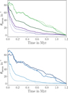 |
Fig. 1 Evolution of average angle θ of star-disk spin with respect to the spin after t = 1.2 Myr (upper panel) and t = 0.5 Myr (lower panel) for various upper and lower limits of the stellar masses. The average angle is computed based on stars that have an age of more than 1.2 Myr at the end of the simulation. Upper panel: Mean average relative angle of orientation with respect to the orientation at t = 1.2 Myr for stars with masses of M*(1.2 Myr) less than 0.2 M⊙, 1 M⊙, and 2 M⊙, shown as light to dark purple lines. Dark to light green lines mark the mean average angle of orientation with respect to the orientation at t = 1.2 Myr for stars with final masses greater than 0.2 M⊙, 1 M⊙, and 2 M⊙. Lower panel: Average mean angle of orientation with respect to the orientation at t = 1.2 Myr for stars with masses in the mass ranges of M* (1.2 Myr) < 0.2 M⊙, 0.2 M⊙ < M*(1.2 Myr) < 1 M⊙, 1 M⊙ < M*(1.2 Myr) < 2 M⊙, and M*(1.2Myr) > 2 M⊙, shown as light to dark blue lines. The upper panel can be directly compared with the results presented in Kuffmeier et al. (2023), while the evolution for mass ranges shown in lower panel is arguably more helpful for comparison with observations of various stellar types. |
3.1 Evolution of the star-disk orientation
To compare the spin evolution over the same extended time interval, we analyzed the spin accrual of the 104 stars that evolved for at least 1.2 Myr in the simulation. The choice of 1.2 Myr was made to allow for a sample of more than 100 stars, while also accounting for infall beyond 1 Myr in the simulation as much as possible. We show the evolution of the average mean in Fig. 1 (and the median in Fig. A.1) angle of the star-disk spin with respect to the spin orientation at 1.2 Myr of the selected 104 stars. We find a clear overall dependency of the spin evolution on the stellar mass, M* at t = 1.2 Myr. On average, the higher M*(t = 1.2 Myr), the longer it takes for the stars to obtain the reference spin orientation at t = 1.2 Myr. This result can be understood in the context of the average mass accretion histories of the stars reported in Kuffmeier et al. (2023). In that work, we found a two-phase accretion process of stars consisting of an initial collapse phase followed by a post-collapse phase. During the post-collapse phase, the star is fed by additional material that is initially not bound to the collapsing progenitor core. The higher the final mass of the star, the larger is the contribution of the post-collapse infall phase. Considering such a process, lower mass stars tend to reach their final spin orientation more quickly than higher mass stars that undergo a prolonged formation phase fueled by infall of material misaligned with respect to the stellar orientation at this point. We also find a kink or a change in the profile of the mean angles within 100 kyr to 200 kyr for all mass bins. We interpret the kink as the transition from the collapse to the post-collapse infall phase, identified in the two-phase accretion scenario.
In the idealized star formation picture, where the star is solely fed by material from an isolated core with uniform rotation, it would be possible to have a prolonged formation time for higher mass stars in the case of sufficiently large cores and under the assumption without fragmentation. However, the star would not show deviations from its rotational axis when it is solely fed with material that has the same rotational axis. Interestingly, the lower mass stars that on average form more rapidly and from a mass reservoir of smaller radial extent also have initially different spins compared to their spin at t = 1.2 Myr.
This effect can be better appreciated in Fig. 2, where we plot the evolution of the spin angle with respect to the spin orientation at t = 1.2 Myr over relative mass accrual instead of time. In contrast to the evolution over time, the plot does not show a clear sign of mass dependency in the spin accrual process in terms of relative mass gain. On average and independent of the mass, the initial spin axis is initially misaligned by about 80° to 90° compared to the spin axis at 1.2 Myr. The stars approach their final spin by an approximate rate of about 8° to 9° per 10% stellar mass accrual. This shows the role of turbulence in the accretion process already during the early collapse stages (Seifried et al. 2012). When the infalling material stems from a turbulent medium, the accretion process is more chaotic in nature (Bate et al. 2010) and, hence, variations in the orientation of the angular momentum vector are expected. Our analysis demonstrates that this is the case in agreement with previous results by Fielding et al. (2015).
We emphasize that the reported dependency applies to the average of the considered mass distributions sample. The distribution of the spin angles at t = 200 kyr (upper panel) and t = 500 kyr (lower panel) in Fig. 3 shows this. For instance, at t = 200 kyr, for stars with M*(1.2 Myr) > 1 M⊙, about 60 % have a spin that is 60° or less from the spin orientation at M*(1.2 Myr). The remaining 40% of the stars with M*(1.2 Myr) > 1 M⊙, have spins that range from angles of 60° up to almost 180°. In fact, almost 20% of the stars with M*(1.2 Myr) > 1 M⊙ have spins at 200 kyr that differ by more than 90° in angle with respect to their spin at t = 1.2 Myr. This implies that there is enough retrograde infall that the entire system can readjust into a configuration where the entire system changes its orientation by more than 90°. We note that these drastic changes apply to the spin of the entire star-disk system. Considering that the disk is typically only ~1% of the stellar mass, we expect the effect of misaligned infall on the disk alone to be even stronger than shown for the proxy of star-disk spin.
Models of infalling gas with different angular momentum vectors onto an existing disk have shown that such infall can lead to a configuration of misaligned inner and outer disks (Thies et al. 2011; Kuffmeier et al. 2021). The results presented above confirm that assuming initial conditions of misaligned infall is justified. In fact, misaligned infall frequently occurs in this simulation especially for stars with masses beyond a few 0.1 M⊙.
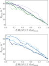 |
Fig. 2 Same as Fig. 1, but for the mean of θ as a function of mean of relative mass accrual instead of time. |
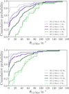 |
Fig. 3 Cumulative probability distribution of changes in stellar spin by angle θ with respect to spin at reference time t = 200 kyr (upper panel) and t = 500 kyr (lower panel). The line colors indicate the same stellar mass thresholds as in the top panel of Fig. 1. |
3.2 Anisotropic accretion and multiplicity
As shown in numerous studies, protostellar accretion happens along accretion channels and sheets (e.g., Offner et al. 2010; Seifried et al. 2012, 2013; Santos-Lima et al. 2012; Joos et al. 2013; Li et al. 2014; Kuffmeier et al. 2017; Heigl et al. 2024). In other words, accretion is anisotropic rather than spherically isotropic. This conclusion generally relies on filamentary accretion shown in the form of 3D visualizations or projection maps that visualize infall-outflow motions at a given radius and there is general consensus about filamentary accretion in the star formation community nowadays. While the reported results are intriguing and informative, a quantitative measure to state the level of (an)isotropy in the accretion process is lacking.
In this work, we have overcome this obstacle by using a quantity that is usually used to measure the (an)isotropy in the context of diffusion processes, namely, fractional anisotropy (FA). It determines whether diffusion occurs rather along a predominant direction (anisotropic case) or whether it occurs unrestricted along all directions (isotropic case). It is defined as
![Mathematical equation: $\[\mathrm{FA}=\sqrt{\frac{1}{2}} \frac{\sqrt{\left(\lambda_1-\lambda_2\right)^2+\left(\lambda_2-\lambda_3\right)^2+\left(\lambda_3-\lambda_1\right)^2}}{\sqrt{\lambda_1^2+\lambda_2^2+\lambda_3^2}},\]$](/articles/aa/full_html/2024/10/aa50410-24/aa50410-24-eq6.png) (3)
(3)
with λ1, λ2 and λ3. being the eigenvalues of the covariance matrix corresponding to the points in the system. FA = 0 corresponds to a perfectly isotropic case, FA = 1 means maximally anisotropic. In our case, the points for the covariance matrix are determined by the components of the angular momentum vector of the accreting tracer particles. We computed FA per accreting mass interval of 0.05 M⊙ for each star. As an example, Fig. 4 shows the evolution of FA for a massive star in the simulation.
Apart from the FA of each mass bin, Fig. 4 also shows whether the star accreted the corresponding mass fraction as a single star or as part of a multiple system. To determine whether the star accretes as a single or multiple star, we analyze the full multiplicity distribution for each snapshot, following the recipe of Kuruwita & Haugbølle (2023) to find all bound systems within a critical distance that we set 2 × 10⁴ au. If the selected star is part of a bound systems within 2 × 10⁴ au during the accrual of Δmp = 0.05 M⊙ at any snapshot, we mark it as accreting as part of a multiple system during that interval (dark blue dots). If it misses a bound member within 2 × 10⁴ au, we mark it as accreting as a single star during that interval (red dots). The plot shows that this star primarily accretes the first half of its mass with other stars in its vicinity, while in the second half it accretes more as a single star. Using the information obtained for all of the selected stars, we can compare the accretion histories of the different stars. This allows us to measure the (an)isotropy of the accreting material for all of the stars (see Sect. 3.2.1), to analyze whether there is an evolutionary trend in the accretion mode (see Sect. 3.2.2), and investigate the influence of multiplicity on the accretion process (see Sect. 3.2.3).
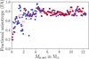 |
Fig. 4 Fractional anisotropy (FA) of the accreting material for a star in the simulation. Each dot represents FA for accrual of a mass bin of 0.05 M⊙. Blue colors mean that the star was part of a multiple system while accreting the corresponding mass, red dots mean that it accreted its material as a single star. The red horizontal lines represent the average of FA over five mass bins, i.e., over 0.25 M⊙. |
3.2.1 (An)isotropy of accretion for all stars
We measured the fractional anisotropy of the accreting material for all 124 stars that evolve to at least 974 kyr over mass accrual of Δmp =0.05 M⊙ as shown for the exemplary star shown in Fig. 4. The lower age limit is used in order to include the reference star that was highlighted as a prime example of late accretion in Kuffmeier et al. (2023). In Fig. 5, we plot the average FA for the 124 stars over the final mass of the corresponding stars. Overall, we find an average of FA = 0.62 ± 0.11 over all stars, which shows that infall generally deviates from isotropic collapse. This corroborates the changes in the orientation of the star-disk spin vector described above. At first sight, the average FA alone does not reveal a striking dependency on stellar mass though the scatter is slightly larger for increasing final mass. We interpret these results as a sign of turbulence generally implying filamentary accretion regardless of the accretion phase and the scatter as a sign of a heterogeneous accretion process in molecular clouds.
3.2.2 Variations between the early and late accretion phases
As highlighted in Kuffmeier et al. (2023), star formation progresses in two stages (arguably with a third stage if accounting for the mass accrual prior to gravitational collapse of the core as part of the process; see Padoan et al. 2020). The first phase is conceptually similar to the classical picture of a collapsing core, while the second phase consists of a sweep-up of material when the star evolves in the GMC. We consider the second phase similar to Bondi-Hoyle-Littleton accretion (Scicluna et al. 2014; Padoan et al. 2024) with an impact parameter of the encountering inflow of material (Dullemond et al. 2019; Kuffmeier et al. 2020). This mode of star formation is also in agreement with observations of accretion streamers that feed star-disk systems with fresh material from the molecular cloud environment (Pineda et al. 2019; Alves et al. 2020; Huang et al. 2020, 2021, 2023; Valdivia-Mena et al. 2022, 2023; Gupta et al. 2023; Cacciapuoti et al. 2024). In particular, a recent analysis of streamer candidates in NGC 1333 by Valdivia-Mena et al. (2024) revealed a fraction of about 40%.
Against this background, we expect the accretion process to be more isotropic in the beginning when the star forms from a local mass reservoir, while the post-collapse phase is more anisotropic. If the initial phase is more isotropic than the late accretion history, we expect that FA at early times is smaller compared to the average FA. Moreover, the contribution of post-collapse infall, tends to increase with increasing final stellar mass. Therefore, we expect this correlation to be more enhanced for higher mass stars that experience a larger contribution of post-collapse infall than lower mass stars that experience only little post-collapse infall.
The evolution of FA for the exemplary star shown in Fig. 4 plot shows such a trend from more isotropic accretion with FA as low as 0.2 for the first accreting 0.1 M⊙ at the beginning to more anisotropic accretion at later stages with FA between 0.7 and about 0.9. To investigate this trend in more detail, we computed the ratio of fractional anisotropy for the first 0.05 M⊙ of accreting mass and the mean of FA given by
![Mathematical equation: $\[\frac{\mathrm{FA}_0}{\overline{\mathrm{FA}}}=\frac{\mathrm{FA}\left(0<\mathrm{M}_{\mathrm{p}, \mathrm{acc}}<0.05 \mathrm{M}_{\odot}\right)}{\overline{\mathrm{FA}}}\]$](/articles/aa/full_html/2024/10/aa50410-24/aa50410-24-eq8.png) (4)
(4)
for each star. We note that we have applied an accretion efficiency factor of 50%, such that only 50% of the cell mass that meets the criteria of accretion is added to the sink mass. This efficiency factor is used to account for mass loss via outflows.
The results are shown in Fig. 6. We find that the mean ratio over all 124 stars is ≈0.88 ± 0.25, hence, it is below 1 (as expected). Applying numpy’s polyfit function to the data points, we fit the data with a straight line with slope ≈-0.036 and offset ≈0.927. The decreasing ratio is a consequence of the larger relative contribution of late infall to the final mass for higher-mass stars. Despite a significant scatter, this analysis confirms that late infall is (on average) more anisotropic than the early collapse phase.
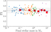 |
Fig. 5 FA of the first Δmp = 0.05 M⊙ with respect to the average FA of the accreting material over the mass at the end of the simulation. The dots show |
![Mathematical equation: $\[\frac{\mathrm{FA}_0}{\overline{\mathrm{FA}}}\]$](/articles/aa/full_html/2024/10/aa50410-24/aa50410-24-eq7.png)
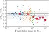 |
Fig. 6 FA of the first 0.05 M⊙ with respect to the average FA of the accreting material over the stellar mass at the end of the simulation. The dots show |
![Mathematical equation: $\[\frac{\mathrm{FA}_0}{\overline{\mathrm{FA}}}\]$](/articles/aa/full_html/2024/10/aa50410-24/aa50410-24-eq9.png)
3.2.3 The role of multiplicity in the accrual of star-disk spin
Considering the mass fraction that stars accrete as a single or as part of multiple stars (Fig. 7), we do not find an immediately striking correlation of FA with multiplicity. For instance, the plot shows two stars with almost identical final masses of about 0.2 M⊙ almost exclusively accreting their mass as single stars, but very different fractional anisotropies of FA > 0.8 and FA < 0.5. Similarly, two stars with final mass of about 0.8 M⊙ that mostly accrete as part of multiple systems have values of FA ≈ 0.4 and FA > 0.8. Nevertheless, there are a few indications for mass-dependent differences in the accretion process. Considering the degree to which each star accreted its material as part of a multiple system or as a single star, the lower panel of Fig. 6 hints at a slightly higher ratio of ![Mathematical equation: $\[\frac{\mathrm{FA}_0}{\overline{\mathrm{FA}}}\]$](/articles/aa/full_html/2024/10/aa50410-24/aa50410-24-eq10.png) for stars that mostly accrete in isolation. Given the relatively low number of about a dozen stars that are categorized as primarily accreting as single stars and the corresponding scatter, the result is only suggestive, but it hints at a scenario where isolated stars are more likely to occur and accrete in a less turbulent medium compared to stars associated with clusters.
for stars that mostly accrete in isolation. Given the relatively low number of about a dozen stars that are categorized as primarily accreting as single stars and the corresponding scatter, the result is only suggestive, but it hints at a scenario where isolated stars are more likely to occur and accrete in a less turbulent medium compared to stars associated with clusters.
The upper panel in Fig. 7 suggests that lower mass stars more often accrete (almost) all of their mass while being classified as part of a multiple system, while higher mass stars tend to accrete part of their mass as single stars. This is in agreement with the result shown for the example star in Fig. 4. This result is also consistent with earlier results of chaotic star formation in an extreme cluster environment of very high densities as considered by Bate (2012). The lowest mass objects, in particular brown dwarfs, are more easily expelled from the cluster through gravitational interactions with other members of the cluster than the more massive stars. The correlation is more visible when plotting the fraction of mass that each star accretes as a single star, ![Mathematical equation: $\[\frac{{n}_{\text {single }}}{n_{\text {single }}+n_{\text {mult }}}\]$](/articles/aa/full_html/2024/10/aa50410-24/aa50410-24-eq11.png) (see top panel in Fig. 8). Fitting the data with a line, we find a very mild positive correlation with mass. The slope is 0.01 and the offset is 0.20. We point out, however, that the average ratio of all stars is
(see top panel in Fig. 8). Fitting the data with a line, we find a very mild positive correlation with mass. The slope is 0.01 and the offset is 0.20. We point out, however, that the average ratio of all stars is ![Mathematical equation: $\[\frac{{n}_{\text {single }}}{n_{\text {single }}+n_{\text {mult }}}\]$](/articles/aa/full_html/2024/10/aa50410-24/aa50410-24-eq12.png) = 0.21 ± 0.27, which shows that there is significant scatter in the data. The scatter appears to be smaller for higher mass stars of final mass above ≈1 M⊙. This reflects the fact that the lower the final mass of the star, the quicker they accrete their mass and the lower the number of mass bins Δmp = 0.05 M⊙ that are considered.
= 0.21 ± 0.27, which shows that there is significant scatter in the data. The scatter appears to be smaller for higher mass stars of final mass above ≈1 M⊙. This reflects the fact that the lower the final mass of the star, the quicker they accrete their mass and the lower the number of mass bins Δmp = 0.05 M⊙ that are considered.
Regardless of the uncertainties and the scatter, the majority of stars accrete their mass with other stars in their vicinity. The histogram of ![Mathematical equation: $\[\frac{{n}_{\text {single }}}{n_{\text {single }}+n_{\text {mult }}}\]$](/articles/aa/full_html/2024/10/aa50410-24/aa50410-24-eq13.png) (bottom panel in Fig. 8) shows that only 17 of the 124 stars (≈ 13.7%) accrete more than half of their mass while being classified as an isolated single star. For stars with final masses less than 0.2 M⊙, the fraction is yet smaller (5/41 ≈ 12.2%), while for stars with masses M* > 0.2 M⊙, the fraction is slightly higher (12/83 ≈ 14.5%).
(bottom panel in Fig. 8) shows that only 17 of the 124 stars (≈ 13.7%) accrete more than half of their mass while being classified as an isolated single star. For stars with final masses less than 0.2 M⊙, the fraction is yet smaller (5/41 ≈ 12.2%), while for stars with masses M* > 0.2 M⊙, the fraction is slightly higher (12/83 ≈ 14.5%).
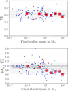 |
Fig. 7 Same as Figs. 5 and 6 except that dots of individual stars are colored according to their evolution as a single star or as part of a multiple system, shown in the top and bottom panels. The redder (bluer) the dot, the higher is the fraction of time that the star evolved as a single star (multiple system) while accreting. |
3.3 Spin in stellar multiples
Using the multiplicity analysis with a cut-off distance of 2 × 10⁴ au and allowing for a maximum of ten stars per system in the search, we find that several stellar systems of order binary or higher have formed by the end of the simulation. In particular, we found a total of 24 systems that consist of three or more stars at the time of t = 1.91 Myr. Using the FA measurement, we analyzed the anisotropy in orientation of the stellar spins in these systems. However, given the small number of stars in the protostellar multiples and the relatively low number of multiple systems, we point out that the following results derived from the analysis of this sample are less robust. They should be understood as indicative and as early constraints for future analyses that are based on larger sample sizes. This is further discussed in Sect. 4.
We plot the fractional anisotropy FA of these systems over the age difference between the oldest and youngest star in the system Δtold–young (Fig. 9). The plot shows two major properties. First, systems with more components tend to have lower values of FA and thereby a more isotropic distribution. Second, systems in which the age difference between the cluster members are larger have lower values of FA than systems consisting of stars that formed within a shorter amount of time.
We hypothesize that this as a consequence of the formation history of the systems. Neighboring stars that form within a few 104 kyr must have formed relatively close to each other likely through core or filament fragmentation in the same region. Therefore, they generally gain their mass and angular momentum from the same reservoir that has the same net angular momentum. Neighboring stars that have age differences of 102 kyr or more, however, formed in different regions and only became neighbors at later stages via dynamical capture. That implies that the stars gained a significant part of their mass and angular momentum from different reservoirs. It is likely that the net angular momentum vectors of these regions pointed in different directions; hence, the stellar spins in systems that originate from dynamical capture are more likely to be misaligned (e.g., Pineda et al. 2012; Brinch et al. 2016; Maureira et al. 2020; Jørgensen et al. 2022). That explains the more isotropic distribution of the spins in these systems compared to systems that formed from the same mass reservoir via core collapse and core fragmentation. To test this hypothesis, we compared the distance between the oldest and youngest member at the time of formation of the youngest member for the systems rold–young(t = t0 (young)) displayed in the top panel of Fig. 9. If the hypothesis is accurate, we expect a larger distance for the systems formed via dynamical capture than for those that formed via fragmentation in the same region. In the middle panel of Fig. 9, we plot the measured FA shown in Fig. 9, but this time over rold–young(t = t0(young)). Keeping in mind the caveat of the very low sample size as shown in the bottom panel of Fig. 9, the plot is in agreement with the expected correlation from the hypothesis that systems forming via dynamical capture tend to have a higher degree of isotropy.
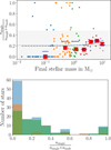 |
Fig. 8 Fraction of output snapshots when individual stars accrete mass as isolated single stars without any neighboring star within a radial distance of 2 × 10⁴ au and total number of output snapshots when accretion is ongoing |
![Mathematical equation: $\[\frac{{n}_{\text {single }}}{n_{\text {single }}+n_{\text {mult }}}\]$](/articles/aa/full_html/2024/10/aa50410-24/aa50410-24-eq14.png)
![Mathematical equation: $\[\frac{{n}_{\text {single }}}{n_{\text {single }}+n_{\text {mult }}}\]$](/articles/aa/full_html/2024/10/aa50410-24/aa50410-24-eq15.png)
4 Discussion
4.1 Limitations of measuring the (an)isotropy of individual stars
The results of stellar spin evolution presented in this paper are obtained by the analysis of accreting Lagrangian tracer particles. Even though the simulation used in this paper has an unprecedented mass resolution and spatial resolution for a global model of a star-forming region and required approximately 100 million core-hours to integrate, the smallest cell size is still 25 au. The downside of this is that we do not resolve accretion disks. In reality, a disk forms and the accretion process likely becomes more anisotropic if the star is predominantly fed from the disk. The tracer particle algorithm allows us to reliably track the trajectory of most of the accreting gas, although the algorithm has known limitations (see Genel et al. 2013). It also serves as a record of tracer particles with a cadence of 5 kyr which is relatively long compared to orbital times of the disk. The presented results can and are supposed to only provide coarse measurements on the orientation of infalling gas onto star-disk systems and should be understood as preliminary constraints on the orientation of primordial and post-collapse infall from the molecular cloud environment. Higher resolution studies are required in the future to further investigate the effects of those events on the disk in detail. However, earlier models considering infall onto disks already demonstrated that infall may lead to instabilities (Lesur et al. 2015; Bae et al. 2015; Kuffmeier et al. 2018; Kuznetsova et al. 2022). Certainly, it will be crucial to account for the presence of the disk self-consistently in future models to obtain a better understanding of the role of infall onto the disk dynamics and the implications for planet formation.
Nonetheless, given the constraints in spatial and temporal resolution, it is remarkable how much valuable information can already be obtained about the potential of infall in modifying the orientation of star-disk systems. With the resolution that is currently available, we are not able to resolve the disk. Therefore, we can confidently conclude that we are indeed tracing the anisotropy of the infalling material, rather than anisotropic disk-induced features. Thus, our finding that the accretion process during the post-collapse infall phase is more anisotropic than during the initial collapse phase is robust.
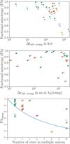 |
Fig. 9 Fractional anisotropy of multiple systems at t ≈ 1.91 Myr after formation of the first star in the simulation. Top panel: fractional anisotropy (FA) versus difference between formation time of oldest and youngest member. Middle panel: FA versus distance between the oldest and youngest member at the formation time of the youngest member. Bottom panel: FA versus number of stars in the corresponding system. The points show the values of the systems and the horizontal bars show the averages for systems with the same number stars. The blue line shows the expectation value for an entirely random distribution computed with 10000 iterations per number of stars using the random sample routine of numpy (Harris et al. 2020). At this point in time, there are 12 triple systems (green points), 6 systems with 4 stars (orange points), 1 system with 5 stars (blue-purple point), 1 system with 6 stars (violet points), 1 system with 8 stars (yellow point), and 3 systems with 10 stars (gray points). |
4.2 Limitations of measuring the (an)isotropy of the star-disk spin of protostellar multiples
There is a serious caveat involved in the analysis based on FA for stellar systems with relatively few members. Although the trend of lower FA, and hence higher isotropy, for increasing Δtold–young is intriguing, FA in multiple systems of only a few members is prone to bias of low number statistics. This can be seen by the expectation value of FA for a given number of N points based on randomized distributions, as shown in Fig. 9. In the future, we aim to measure the spin of stars in clusters by carrying out simulations of a larger GMC. Although the domain and sample size of the underlying simulations analyzed in this paper is too small to derive definite conclusions on the (an)isotropy of the stellar spin in clusters, we expect that FA will be a good metric, when comparing the spin orientation of clusters with more members. Figure A.10 shows that the expectation value drops to <0.2 for N > 100 members, which illustrates the reduced role of small number statistics for larger clusters with a higher number of members. We emphasize that the analysis of the anisotropy of the accretion process in Sec. 3.2 is practically unaffected by this bias because the considered mass bins of 0.05 M⊙ typically contain ~ 103 tracer particles.
4.3 Implications for interpretation of disk observations
Star formation models that take into account the turbulent dynamics in molecular clouds show that post-collapse infall is a common feature of star formation, especially for stars with final masses beyond a few 0.1 M⊙ (Smith et al. 2011; Pelkonen et al. 2021; Kuffmeier et al. 2023). In addition, the analysis presented in this paper demonstrates that infall is anisotropic. Such prolonged histories of mass accretion through anisotropic infall are consistent with recent observations of accretion streamers such as Per-emb-2 (Pineda et al. 2019), Per-emb-50 (Valdivia-Mena et al. 2022), Barnard 5 (Valdivia-Mena et al. 2023), L1455 IRS1 (Chou et al. 2016), IRAS 16544-1604 (Kido et al. 2023), IRAS 16253-2429 (Aso et al. 2023), DK Cha (Harada et al. 2023), GGD 27-MM1 (Fernández-López et al. 2023), BHB 1 (Alves et al. 2020), HL Tau (Yen et al. 2019; Garufi et al. 2021), M512 (Grant et al. 2021; Cacciapuoti et al. 2024), AB Aurigae (Grady et al. 1999), SU Aurigae (Akiyama et al. 2019; Ginski et al. 2021; Labdon et al. 2023), S Cra (Gupta et al. 2023), RU Lup (Huang et al. 2020), GM Aur (Huang et al. 2021), or DR Tau (Huang et al. 2023).
Moreover, our results show that infall is typically misaligned with respect to the orientation of the star-disk system (see also Pelkonen et al. 2024). This important result implies that the assumption of misaligned infall in previous models (Thies et al. 2011; Kuffmeier et al. 2021) is justified, which provides strong support for the formation of misaligned disks via late infall traceable as shadows in scattered light observations of disks (Krieger et al. 2024). A missing step in the near future is to combine the two approaches by increasing the resolution of the large-scale models sufficiently to resolve individual infall events and thereby to study how they affect the primordial disk and how often this type of infall can lead to misaligned disk-systems. This require a new generation of highly scalable codes that can support the volume and dynamic range needed. We are currently preparing zoom-in simulations using the exa-scale ready code DISPATCH (Nordlund et al. 2018) to investigate individual infall events with high enough refinement to resolve the disk during infall events. Such simulations will allow us to investigate how existing star-disk systems respond to anisotropic misaligned infall. By investigating a sample of events, it will be possible to set further statistical constraints on the probability and characteristic lifetimes of misaligned disk configurations.
5 Conclusion
In this paper, we study the role of infall by analyzing data from a 3D simulation of a molecular cloud of (4 pc)3 in volume that was carried out with the RAMSES code. Inspired by previous results that have demonstrated the possibility of mass accretion after the initial collapse phase via post-collapse infall, we study the effect of infall on the orientation of star-disk systems. Measuring the angular momentum vector of tracer particles at the snapshot prior to accretion onto a star, we find that infall is typically misaligned with respect to the current orientation of the star-disk system. As the infall events can contribute a significant mass fraction to the final mass of the star (~10%), misaligned infall can drastically reorient the rotational axis of the star-disk system. We also find that (on average) it takes more time for a star-disk system to reach its final spin orientation, the larger its final mass. This result is consistent and a direct consequence of the mass accretion histories that, on average, the duration of infall lasts longer for increasing final mass of a star.
Our results show that the orientation of a star-disk system is tightly coupled to the amount of material that is infalling. In fact, when normalizing the spin orientation of star-disk systems to the accreting mass relative to the final mass, we find that the spin of the star evolves independently of the final stellar mass from an initial misalignment with respect to its final orientation of ≈80°, roughly at a rate of 8° per ΔM = 0.1 M*,flnal.
We did not resolve the disks in the underlying simulations, but we did indeed see significant changes in the orientation during infall for mass infall, which contributes (~10%) to the final mass of the star. Unless angular momentum transport is very efficient at the 100 au to 500 au scale, we expect to see a significant reconfiguration of the disk – even for infall events of relatively little mass with respect to the final stellar mass (≲1%), considering that the disk itself only has a mass of ~1% of the host star. We will investigate the effect of infall on the configuration and orientation of the disk further in upcoming zoom-in simulations.
We analyzed whether stars in the simulation accreted as single stars or as part of multiple systems. Stars and brown dwarfs with final masses ≲0.2 M⊙ are more likely to form and accrete as members of multiple systems and small clusters, before the ejection from the accretion reservoir (i.e., the cluster) causes starvation and the end of the accretion process. Low-mass stars and brown dwarfs that happen to encounter another accretion reservoir in the molecular cloud grow further in mass, typically beyond 0.2 M⊙. Stars with masses between 0.2 to 1 M⊙ are more likely to accrete as single stars throughout their formation and evolution. However, most stars are part of multiple systems or near other stars during most of their accretion. Stars with final masses ≳ 1 M⊙ have, on average, prolonged accretion times due to the higher probability of post-collapse infall through Bondi-Hoyle-Littleton accretion. As a result of the longer accretion history, they often accrete a small fraction of their mass alone though they spend most of their accretion time as part of multiple systems.
We also provide constraints on the anisotropy of the accretion process. To do so, we adapted the measure of fractional anisotropy (FA) that is typically used to give an estimate of the (an)isotropy of a diffusion process. We find a mean FA of ≈0.6 averaged over 124 stars that reach an age of ≈1 Myr or more, which means that infall and thereby accretion is anisotropic. There is no dependency of the average fractional anisotropy of accreting stars on the final stellar mass.
A comparison of the ratio of FA for the initial 0.05 M⊙ with the mean of FA shows that the accretion process is initially more isotropic compared to later stages. We also find a trend that the ratio decreases with increasing final stellar mass. This is consistent with a mode of accretion, where the star forms from the initial collapse of a dense gas followed by more anisotropic accretion that is funneled by infall through accretion streamers.
Acknowledgements
The authors thank the referee and the editor for helpful, constructive feedback and suggestions on how to improve the manuscript. MK thanks Andrew Winter for pointing out missing references and a fruitful dialogue on the presumably underestimated contribution of post-collapse infall on disk formation in the context of MK’s previous work and a submitted manuscript on the origin of Class II disks (Winter et al. 2024). MK also acknowledges helpful inspiration through the kick-off meeting of the COST action “CA22133 – The birth of solar systems (PLANETS)”, in particular to Jiri Zak for helpful feedback on an earlier version of the manuscript. The research of MK is supported by H2020 Marie Skłodowska-Curie Actions (897524) and a Carlsberg Reintegration Fellowship (CF22-1014). D. S.-C. is supported by an NSF Astronomy and Astrophysics Postdoctoral Fellowship under award AST-2102405. The Tycho HPC facility at the University of Copenhagen, supported by research grants from the Carlsberg, Novo, and Villum foundations, was used for carrying out the simulations, the analysis, and the long-term storage of the results.
Appendix A Mean and median of spin angles over median and mean masses
In complement to the plots shown in the main part of the paper, we also show the median of angle θ over time in Fig. A.1, the median of angle θ over the median of relative mass accrual in Fig. A.2, the mean of angle θ over the median of relative mass accrual in Fig. A.3, as well as the median of angle θ over the mean of relative mass accrual in Fig. A.4. Moreover, we show fractional anisotropy over the mean and median of the difference in formation time between the system members in Fig. A.5, as well as FA over the mean and median of the difference in relative distance in Fig. A.6. Figure A.7 to Fig. A.9 show FA over the relative distance Δrold–i with respect to the individual members. Finally, Fig. A.10 shows the mean value of FA for multiple systems of n members based on a random distribution of 10000 iterations.
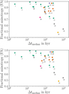 |
Fig. A.5 Fractional anisotropy of multiple systems shown in Fig. 9, but plotted over the mean (upper panel) and median (lower panel) of the difference in formation time of the members in the systems. |
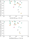 |
Fig. A.6 Fractional anisotropy of multiple systems shown in Fig. 9, but plotted over the mean (upper panel) and median (lower panel) of the distance to the oldest component. |
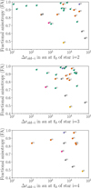 |
Fig. A.7 Fractional anisotropy (FA) measured at t = 1.91 Myr for the 24 systems shown in Fig. 9, but plotted over distance between the oldest member (1) and member i at the formation time of member i from i = 2 (second oldest star in the system; top panel) to i = 4 (4th oldest star in the system; bottom panel). |
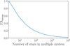 |
Fig. A.10 Expectation value of fractional anisotropy FA for a random distribution of n vectors. The expectation value is computed over 10000 iterations per system with n vectors. |
References
- Akiyama, E., Vorobyov, E. I., Liu, H. B., et al. 2019, AJ, 157, 165 [NASA ADS] [CrossRef] [Google Scholar]
- Albrecht, S. H., Dawson, R. I., & Winn, J. N. 2022, PASP, 134, 082001 [NASA ADS] [CrossRef] [Google Scholar]
- Alves, F. O., Cleeves, L. I., Girart, J. M., et al. 2020, ApJ, 904, L6 [NASA ADS] [CrossRef] [Google Scholar]
- Andre, P., Ward-Thompson, D., & Barsony, M. 1993, ApJ, 406, 122 [NASA ADS] [CrossRef] [Google Scholar]
- Arce, H. G., Borkin, M. A., Goodman, A. A., Pineda, J. E., & Halle, M. W. 2010, ApJ, 715, 1170 [NASA ADS] [CrossRef] [Google Scholar]
- Aso, Y., Kwon, W., Ohashi, N., et al. 2023, ApJ, 954, 101 [NASA ADS] [CrossRef] [Google Scholar]
- Avenhaus, H., Quanz, S. P., Schmid, H. M., et al. 2017, AJ, 154, 33 [Google Scholar]
- Bae, J., Hartmann, L., & Zhu, Z. 2015, ApJ, 805, 15 [NASA ADS] [CrossRef] [Google Scholar]
- Bate, M. R. 2012, MNRAS, 419, 3115 [NASA ADS] [CrossRef] [Google Scholar]
- Bate, M. R. 2018, MNRAS, 475, 5618 [Google Scholar]
- Bate, M. R., Lodato, G., & Pringle, J. E. 2010, MNRAS, 401, 1505 [NASA ADS] [CrossRef] [Google Scholar]
- Benisty, M., Stolker, T., Pohl, A., et al. 2017, A&A, 597, A42 [NASA ADS] [CrossRef] [EDP Sciences] [Google Scholar]
- Benisty, M., Juhász, A., Facchini, S., et al. 2018, A&A, 619, A171 [NASA ADS] [CrossRef] [EDP Sciences] [Google Scholar]
- Boehler, Y., Ricci, L., Weaver, E., et al. 2018, ApJ, 853, 162 [Google Scholar]
- Brinch, C., Jørgensen, J. K., Hogerheijde, M. R., Nelson, R. P., & Gressel, O. 2016, ApJ, 830, L16 [Google Scholar]
- Cacciapuoti, L., Macias, E., Gupta, A., et al. 2024, A&A, 682, A61 [NASA ADS] [CrossRef] [EDP Sciences] [Google Scholar]
- Casassus, S., Marino, S., Pérez, S., et al. 2015, ApJ, 811, 92 [Google Scholar]
- Casassus, S., Avenhaus, H., Pérez, S., et al. 2018, MNRAS, 477, 5104 [NASA ADS] [CrossRef] [Google Scholar]
- Cheng, Y., Lu, X., Sanhueza, P., et al. 2024, ApJ, 967, 56 [Google Scholar]
- Chou, H.-G., Yen, H.-W., Koch, P. M., & Guilloteau, S. 2016, ApJ, 823, 151 [NASA ADS] [CrossRef] [Google Scholar]
- Cuello, N., Ménard, F., & Price, D. J. 2023, Eur. Phys. J. Plus, 138, 11 [NASA ADS] [CrossRef] [Google Scholar]
- Dullemond, C. P., Küffmeier, M., Goicovic, F., et al. 2019, A&A, 628, A20 [NASA ADS] [CrossRef] [EDP Sciences] [Google Scholar]
- Federrath, C., Schrön, M., Banerjee, R., & Klessen, R. S. 2014, ApJ, 790, 128 [NASA ADS] [CrossRef] [Google Scholar]
- Fernández-López, M., Girart, J. M., López-Vázquez, J. A., et al. 2023, ApJ, 956, 82 [CrossRef] [Google Scholar]
- Fielding, D. B., McKee, C. F., Socrates, A., Cunningham, A. J., & Klein, R. I. 2015, MNRAS, 450, 3306 [NASA ADS] [CrossRef] [Google Scholar]
- Garufi, A., Podio, L., Codella, C., et al. 2021, A&A, 645, A145 [EDP Sciences] [Google Scholar]
- Garufi, A., Dominik, C., Ginski, C., et al. 2022, A&A, 658, A137 [NASA ADS] [CrossRef] [EDP Sciences] [Google Scholar]
- Garufi, A., Ginski, C., van Holstein, R. G., et al. 2024, A&A, 685, A53 [NASA ADS] [CrossRef] [EDP Sciences] [Google Scholar]
- Genel, S., Vogelsberger, M., Nelson, D., et al. 2013, MNRAS, 435, 1426 [NASA ADS] [CrossRef] [Google Scholar]
- Ginski, C., Facchini, S., Huang, J., et al. 2021, ApJ, 908, L25 [NASA ADS] [CrossRef] [Google Scholar]
- Grady, C. A., Woodgate, B., Bruhweiler, F. C., et al. 1999, ApJ, 523, L151 [NASA ADS] [CrossRef] [Google Scholar]
- Grant, S. L., Espaillat, C. C., Wendeborn, J., et al. 2021, ApJ, 913, 123 [NASA ADS] [CrossRef] [Google Scholar]
- Gupta, A., Miotello, A., Manara, C. F., et al. 2023, A&A, 670, L8 [NASA ADS] [CrossRef] [EDP Sciences] [Google Scholar]
- Harada, N., Tokuda, K., Yamasaki, H., et al. 2023, ApJ, 945, 63 [NASA ADS] [CrossRef] [Google Scholar]
- Harris, C. R., Millman, K. J., van der Walt, S. J., et al. 2020, Nature, 585, 357 [NASA ADS] [CrossRef] [Google Scholar]
- Haugbølle, T., Padoan, P., & Nordlund, Å. 2018, ApJ, 854, 35 [CrossRef] [Google Scholar]
- Heigl, S., Hoemann, E., & Burkert, A. 2024, A&A, 686, A246 [NASA ADS] [CrossRef] [EDP Sciences] [Google Scholar]
- Holt, J. R. 1893, A&A, 12, 646 [Google Scholar]
- Huang, J., Andrews, S. M., Öberg, K. I., et al. 2020, ApJ, 898, 140 [NASA ADS] [CrossRef] [Google Scholar]
- Huang, J., Bergin, E. A., Öberg, K. I., et al. 2021, ApJS, 257, 19 [NASA ADS] [CrossRef] [Google Scholar]
- Huang, J., Bergin, E. A., Bae, J., Benisty, M., & Andrews, S. M. 2023, ApJ, 943, 107 [NASA ADS] [CrossRef] [Google Scholar]
- Itoh, Y., Oasa, Y., Kudo, T., et al. 2014, Res. Astron. Astrophys., 14, 1438 [CrossRef] [Google Scholar]
- Jensen, S. S., & Haugbølle, T. 2018, MNRAS, 474, 1176 [Google Scholar]
- Jensen, S. S., Spezzano, S., Caselli, P., Grassi, T., & Haugbølle, T. 2023, A&A, 675, A34 [NASA ADS] [CrossRef] [EDP Sciences] [Google Scholar]
- Joos, M., Hennebelle, P., Ciardi, A., & Fromang, S. 2013, A&A, 554, A17 [NASA ADS] [CrossRef] [EDP Sciences] [Google Scholar]
- Jørgensen, J. K., Kuruwita, R. L., Harsono, D., et al. 2022, Nature, 606, 272 [CrossRef] [Google Scholar]
- Keppler, M., Penzlin, A., Benisty, M., et al. 2020, A&A, 639, A62 [NASA ADS] [CrossRef] [EDP Sciences] [Google Scholar]
- Kido, M., Takakuwa, S., Saigo, K., et al. 2023, ApJ, 953, 190 [NASA ADS] [CrossRef] [Google Scholar]
- Kraus, S., Kreplin, A., Young, A. K., et al. 2020, Science, 369, 1233 [NASA ADS] [CrossRef] [Google Scholar]
- Krieger, A., Kuffmeier, M., Reissl, S., et al. 2024, A&A, 686, A111 [NASA ADS] [CrossRef] [EDP Sciences] [Google Scholar]
- Kuffmeier, M. 2024, arXiv e-prints [arXiv:2406.10901] [Google Scholar]
- Kuffmeier, M., Haugbølle, T., & Nordlund, Å. 2017, ApJ, 846, 7 [NASA ADS] [CrossRef] [Google Scholar]
- Kuffmeier, M., Frimann, S., Jensen, S. S., & Haugbølle, T. 2018, MNRAS, 475, 2642 [NASA ADS] [CrossRef] [Google Scholar]
- Kuffmeier, M., Goicovic, F. G., & Dullemond, C. P. 2020, A&A, 633, A3 [NASA ADS] [CrossRef] [EDP Sciences] [Google Scholar]
- Kuffmeier, M., Dullemond, C. P., Reissl, S., & Goicovic, F. G. 2021, A&A, 656, A161 [NASA ADS] [CrossRef] [EDP Sciences] [Google Scholar]
- Kuffmeier, M., Jensen, S. S., & Haugbølle, T. 2023, Eur. Phys. J. Plus, 138, 272 [NASA ADS] [CrossRef] [Google Scholar]
- Kuruwita, R. L., & Haugbølle, T. 2023, A&A, 674, A196 [NASA ADS] [CrossRef] [EDP Sciences] [Google Scholar]
- Kuznetsova, A., Bae, J., Hartmann, L., & Mac Low, M.-M. 2022, ApJ, 928, 92 [NASA ADS] [CrossRef] [Google Scholar]
- Labdon, A., Kraus, S., Davies, C. L., et al. 2023, A&A, 678, A6 [NASA ADS] [CrossRef] [EDP Sciences] [Google Scholar]
- Lada, C. J. 1987, in Star Forming Regions, 115, eds. M. Peimbert, & J. Jugaku, 1 [Google Scholar]
- Lada, C. J., & Wilking, B. A. 1984, ApJ, 287, 610 [NASA ADS] [CrossRef] [Google Scholar]
- Larson, R. B. 1969, MNRAS, 145, 271 [Google Scholar]
- Lebreuilly, U., Vallucci-Goy, V., Guillet, V., Lombart, M., & Marchand, P. 2023, MNRAS, 518, 3326 [Google Scholar]
- Lesur, G., Hennebelle, P., & Fromang, S. 2015, A&A, 582, L9 [NASA ADS] [CrossRef] [EDP Sciences] [Google Scholar]
- Li, Z.-Y., Krasnopolsky, R., Shang, H., & Zhao, B. 2014, ApJ, 793, 130 [Google Scholar]
- Marino, S., Perez, S., & Casassus, S. 2015, ApJ, 798, L44 [Google Scholar]
- Maureira, M. J., Pineda, J. E., Segura-Cox, D. M., et al. 2020, ApJ, 897, 59 [NASA ADS] [CrossRef] [Google Scholar]
- McLaughlin, D. B. 1924, ApJ, 60, 22 [Google Scholar]
- Morii, K., Sanhueza, P., Nakamura, F., et al. 2023, ApJ, 950, 148 [NASA ADS] [CrossRef] [Google Scholar]
- Muro-Arena, G. A., Benisty, M., Ginski, C., et al. 2020, A&A, 635, A121 [NASA ADS] [CrossRef] [EDP Sciences] [Google Scholar]
- Nealon, R., Dipierro, G., Alexander, R., Martin, R. G., & Nixon, C. 2018, MNRAS, 481, 20 [Google Scholar]
- Nealon, R., Cuello, N., Gonzalez, J.-F., et al. 2020, MNRAS, 499, 3857 [Google Scholar]
- Nordlund, Å., Ramsey, J. P., Popovas, A., & Küffmeier, M. 2018, MNRAS, 477, 624 [NASA ADS] [CrossRef] [Google Scholar]
- Offner, S. S. R., Kratter, K. M., Matzner, C. D., Krumholz, M. R., & Klein, R. I. 2010, ApJ, 725, 1485 [Google Scholar]
- Offner, S. S. R., Moe, M., Kratter, K. M., et al. 2023, in Astronomical Society of the Pacific Conference Series, 534, Protostars and Planets VII, eds. S. Inutsuka, Y. Aikawa, T. Muto, K. Tomida, & M. Tamura, 275 [Google Scholar]
- Padoan, P., Haugbølle, T., & Nordlund, Å. 2014, ApJ, 797, 32 [Google Scholar]
- Padoan, P., Pan, L., Juvela, M., Haugbølle, T., & Nordlund, Å. 2020, ApJ, 900, 82 [NASA ADS] [CrossRef] [Google Scholar]
- Padoan, P., Pan, L., Pelkonen, V.-M., Haugboelle, T., & Nordlund, A. 2024, arXiv e-prints [arXiv:2405.07334] [Google Scholar]
- Pelkonen, V. M., Padoan, P., Haugbølle, T., & Nordlund, Å. 2021, MNRAS, 504, 1219 [NASA ADS] [CrossRef] [Google Scholar]
- Pelkonen, V.-M., Padoan, P., Juvela, M., Haugbølle, T., & Nordlund, Å. 2024, arXiv e-prints [arXiv:2405.06520] [Google Scholar]
- Pineda, J. E., Maury, A. J., Fuller, G. A., et al. 2012, A&A, 544, L7 [NASA ADS] [CrossRef] [EDP Sciences] [Google Scholar]
- Pineda, J. E., Zhao, B., Schmiedeke, A., et al. 2019, ApJ, 882, 103 [NASA ADS] [CrossRef] [Google Scholar]
- Pineda, J. E., Arzoumanian, D., Andre, P., et al. 2023, in Astronomical Society of the Pacific Conference Series, 534, Protostars and Planets VII, eds. S. Inutsuka, Y. Aikawa, T. Muto, K. Tomida, & M. Tamura, 233 [Google Scholar]
- Pinilla, P., Benisty, M., de Boer, J., et al. 2018, ApJ, 868, 85 [NASA ADS] [CrossRef] [Google Scholar]
- Rossiter, R. A. 1924, ApJ, 60, 15 [Google Scholar]
- Sanhueza, P., Contreras, Y., Wu, B., et al. 2019, ApJ, 886, 102 [Google Scholar]
- Santos-Lima, R., de Gouveia Dal Pino, E. M., & Lazarian, A. 2012, ApJ, 747, 21 [NASA ADS] [CrossRef] [Google Scholar]
- Scicluna, P., Rosotti, G., Dale, J. E., & Testi, L. 2014, A&A, 566, L3 [NASA ADS] [CrossRef] [EDP Sciences] [Google Scholar]
- Seifried, D., Banerjee, R., Pudritz, R. E., & Klessen, R. S. 2012, MNRAS, 423, L40 [NASA ADS] [CrossRef] [Google Scholar]
- Seifried, D., Banerjee, R., Pudritz, R. E., & Klessen, R. S. 2013, MNRAS, 432, 3320 [NASA ADS] [CrossRef] [Google Scholar]
- Shu, F. H. 1977, ApJ, 214, 488 [Google Scholar]
- Smallwood, J. L., Nealon, R., Cuello, N., Dong, R., & Booth, R. A. 2024, MNRAS, 527, 2094 [Google Scholar]
- Smith, R. J., Glover, S. C. O., Bonnell, I. A., Clark, P. C., & Klessen, R. S. 2011, MNRAS, 411, 1354 [NASA ADS] [CrossRef] [Google Scholar]
- Stadler, J., Benisty, M., Izquierdo, A., et al. 2023, A&A, 670, L1 [NASA ADS] [CrossRef] [EDP Sciences] [Google Scholar]
- Stolker, T., Dominik, C., Avenhaus, H., et al. 2016, A&A, 595, A113 [NASA ADS] [CrossRef] [EDP Sciences] [Google Scholar]
- Takaishi, D., Tsukamoto, Y., & Suto, Y. 2020, MNRAS, 492, 5641 [NASA ADS] [CrossRef] [Google Scholar]
- Terebey, S., Shu, F. H., & Cassen, P. 1984, ApJ, 286, 529 [Google Scholar]
- Thalmann, C., Janson, M., Garufi, A., et al. 2016, ApJ, 828, L17 [Google Scholar]
- Thies, I., Kroupa, P., Goodwin, S. P., Stamatellos, D., & Whitworth, A. P. 2011, MNRAS, 417, 1817 [NASA ADS] [CrossRef] [Google Scholar]
- Uyama, T., Currie, T., Christiaens, V., et al. 2020, ApJ, 900, 135 [NASA ADS] [CrossRef] [Google Scholar]
- Valdivia-Mena, M. T., Pineda, J. E., Segura-Cox, D. M., et al. 2022, A&A, 667, A12 [NASA ADS] [CrossRef] [EDP Sciences] [Google Scholar]
- Valdivia-Mena, M. T., Pineda, J. E., Segura-Cox, D. M., et al. 2023, A&A, 677, A92 [NASA ADS] [CrossRef] [EDP Sciences] [Google Scholar]
- Valdivia-Mena, M. T., Pineda, J. E., Caselli, P., et al. 2024, A&A, 687, A71 [NASA ADS] [CrossRef] [EDP Sciences] [Google Scholar]
- Winter, A. J., & Haworth, T. J. 2022, Eur. Phys. J. Plus, 137, 1132 [NASA ADS] [CrossRef] [Google Scholar]
- Winter, A. J., Benisty, M., & Andrews, S. M. 2024, arXiv e-prints [arXiv:2405.08451] [Google Scholar]
- Yen, H.-W., Gu, P.-G., Hirano, N., et al. 2019, ApJ, 880, 69 [NASA ADS] [CrossRef] [Google Scholar]
- Zhao, B., Tomida, K., Hennebelle, P., et al. 2020, Space Sci. Rev., 216, 43 [CrossRef] [Google Scholar]
- Zhu, Z. 2019, MNRAS, 483, 4221 [Google Scholar]
- Zurlo, A., Weber, P., Pérez, S., et al. 2024, A&A, 686, A309 [NASA ADS] [CrossRef] [EDP Sciences] [Google Scholar]
A recipe to track the stellar spin following the method presented in (Federrath et al. 2014) was recently implemented Dalsgaard et al., in prep. However, the high-resolution run (root-grid of 5123 cells) that was used for the analysis in this paper was carried out before the recipe was implemented.
All Figures
|
Fig. 1 Evolution of average angle θ of star-disk spin with respect to the spin after t = 1.2 Myr (upper panel) and t = 0.5 Myr (lower panel) for various upper and lower limits of the stellar masses. The average angle is computed based on stars that have an age of more than 1.2 Myr at the end of the simulation. Upper panel: Mean average relative angle of orientation with respect to the orientation at t = 1.2 Myr for stars with masses of M*(1.2 Myr) less than 0.2 M⊙, 1 M⊙, and 2 M⊙, shown as light to dark purple lines. Dark to light green lines mark the mean average angle of orientation with respect to the orientation at t = 1.2 Myr for stars with final masses greater than 0.2 M⊙, 1 M⊙, and 2 M⊙. Lower panel: Average mean angle of orientation with respect to the orientation at t = 1.2 Myr for stars with masses in the mass ranges of M* (1.2 Myr) < 0.2 M⊙, 0.2 M⊙ < M*(1.2 Myr) < 1 M⊙, 1 M⊙ < M*(1.2 Myr) < 2 M⊙, and M*(1.2Myr) > 2 M⊙, shown as light to dark blue lines. The upper panel can be directly compared with the results presented in Kuffmeier et al. (2023), while the evolution for mass ranges shown in lower panel is arguably more helpful for comparison with observations of various stellar types. |
| In the text | |
|
Fig. 2 Same as Fig. 1, but for the mean of θ as a function of mean of relative mass accrual instead of time. |
| In the text | |
|
Fig. 3 Cumulative probability distribution of changes in stellar spin by angle θ with respect to spin at reference time t = 200 kyr (upper panel) and t = 500 kyr (lower panel). The line colors indicate the same stellar mass thresholds as in the top panel of Fig. 1. |
| In the text | |
|
Fig. 4 Fractional anisotropy (FA) of the accreting material for a star in the simulation. Each dot represents FA for accrual of a mass bin of 0.05 M⊙. Blue colors mean that the star was part of a multiple system while accreting the corresponding mass, red dots mean that it accreted its material as a single star. The red horizontal lines represent the average of FA over five mass bins, i.e., over 0.25 M⊙. |
| In the text | |
|
Fig. 5 FA of the first Δmp = 0.05 M⊙ with respect to the average FA of the accreting material over the mass at the end of the simulation. The dots show |
| In the text | |
|
Fig. 6 FA of the first 0.05 M⊙ with respect to the average FA of the accreting material over the stellar mass at the end of the simulation. The dots show |
| In the text | |
|
Fig. 7 Same as Figs. 5 and 6 except that dots of individual stars are colored according to their evolution as a single star or as part of a multiple system, shown in the top and bottom panels. The redder (bluer) the dot, the higher is the fraction of time that the star evolved as a single star (multiple system) while accreting. |
| In the text | |
|
Fig. 8 Fraction of output snapshots when individual stars accrete mass as isolated single stars without any neighboring star within a radial distance of 2 × 10⁴ au and total number of output snapshots when accretion is ongoing |
| In the text | |
|
Fig. 9 Fractional anisotropy of multiple systems at t ≈ 1.91 Myr after formation of the first star in the simulation. Top panel: fractional anisotropy (FA) versus difference between formation time of oldest and youngest member. Middle panel: FA versus distance between the oldest and youngest member at the formation time of the youngest member. Bottom panel: FA versus number of stars in the corresponding system. The points show the values of the systems and the horizontal bars show the averages for systems with the same number stars. The blue line shows the expectation value for an entirely random distribution computed with 10000 iterations per number of stars using the random sample routine of numpy (Harris et al. 2020). At this point in time, there are 12 triple systems (green points), 6 systems with 4 stars (orange points), 1 system with 5 stars (blue-purple point), 1 system with 6 stars (violet points), 1 system with 8 stars (yellow point), and 3 systems with 10 stars (gray points). |
| In the text | |
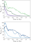 |
Fig. A.1 Same as Fig. 1, but for the median of θ. |
| In the text | |
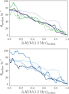 |
Fig. A.2 Same as Fig. 1, but for the median of θ over median of relative mass accrual. |
| In the text | |
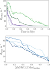 |
Fig. A.3 Same as Fig. 1, but for the mean of θ over median of relative mass accrual. |
| In the text | |
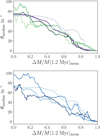 |
Fig. A.4 Same as Fig. 1, but for the median of θ over mean of relative mass accrual. |
| In the text | |
|
Fig. A.5 Fractional anisotropy of multiple systems shown in Fig. 9, but plotted over the mean (upper panel) and median (lower panel) of the difference in formation time of the members in the systems. |
| In the text | |
|
Fig. A.6 Fractional anisotropy of multiple systems shown in Fig. 9, but plotted over the mean (upper panel) and median (lower panel) of the distance to the oldest component. |
| In the text | |
|
Fig. A.7 Fractional anisotropy (FA) measured at t = 1.91 Myr for the 24 systems shown in Fig. 9, but plotted over distance between the oldest member (1) and member i at the formation time of member i from i = 2 (second oldest star in the system; top panel) to i = 4 (4th oldest star in the system; bottom panel). |
| In the text | |
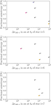 |
Fig. A.8 Same as Fig. A.7, but for the fifth to seventh member. |
| In the text | |
 |
Fig. A.9 Same as Fig. A.7, but for the eighth to tenth member. |
| In the text | |
|
Fig. A.10 Expectation value of fractional anisotropy FA for a random distribution of n vectors. The expectation value is computed over 10000 iterations per system with n vectors. |
| In the text | |
Current usage metrics show cumulative count of Article Views (full-text article views including HTML views, PDF and ePub downloads, according to the available data) and Abstracts Views on Vision4Press platform.
Data correspond to usage on the plateform after 2015. The current usage metrics is available 48-96 hours after online publication and is updated daily on week days.
Initial download of the metrics may take a while.