| Issue |
A&A
Volume 690, October 2024
|
|
|---|---|---|
| Article Number | A87 | |
| Number of page(s) | 15 | |
| Section | Astrophysical processes | |
| DOI | https://doi.org/10.1051/0004-6361/202450122 | |
| Published online | 01 October 2024 | |
Quiescent black hole X-ray binaries as multi-messenger sources
Laboratoire d’Annecy-le-Vieux de Physique Théorique (LAPTh), USMB, CNRS, 74940 Annecy, France
Received:
25
March
2024
Accepted:
22
July
2024
Abstract
The origin of Galactic cosmic rays (CRs) is unknown even though they have traditionally been connected to supernovae based on energetic arguments. In the past decades, Galactic black holes in X-ray binaries (BHXBs) have been proposed as candidate sources of CRs, which revises the CR paradigm. BHXBs launch two relativistic jets during their outbursts, but recent observations suggested that these jets may be launched even during quiescence. A0620−00 is a well-studied object that shows indications of jet emission. We study the simultaneous radio-to-X-ray spectrum of this source that was detected while the source was in quiescence to better constrain the jet dynamics. Because most BHXBs spend their lifetimes in quiescence (qBHXBs), we used the jet dynamics of A0620−00 to study a population of 105 such sources distributed throughout the Galactic disc, and a further 104 sources that are located in the boxy bulge around the Galactic centre. While the contribution to the CR spectrum is suppressed, we find that the cumulative intrinsic emission of qBHXBs from both the boxy bulge and from the Galactic disc adds to the diffuse emission that various facilities detected from radio to TeV γ rays. We examined the contribution of qBHXBs to the Galactic diffuse emission and investigated the possibility of SKA, INTEGRAL, and CTAO to detect individual sources in the future. Finally, we compare the predicted neutrino flux to the recently presented Galactic diffuse neutrino emission by IceCube.
Key words: acceleration of particles / Galaxy: disk / gamma rays: diffuse background / X-rays: diffuse background
© The Authors 2024
 Open Access article, published by EDP Sciences, under the terms of the Creative Commons Attribution License (https://creativecommons.org/licenses/by/4.0), which permits unrestricted use, distribution, and reproduction in any medium, provided the original work is properly cited.
This article is published in open access under the Subscribe to Open model. This email address is being protected from spambots. You need JavaScript enabled to view it. to support open access publication.
1. Introduction
Cosmic rays (CRs) are charged particles with an extraterrestrial origin. Despite decades of research, we still lack a full understanding of the CR sources and the physical mechanism behind their acceleration. When CRs accelerate, they reach high energies that allow the emission of γ rays. On the one hand, leptonic CRs can upscatter background radiation to γ rays, and on the other hand, hadronic CRs can interact inelastically with background photons and/or gas to produce secondary particles, such as γ rays and neutrinos (Mannheim & Schlickeiser 1994). When Galactic CRs propagate in the interstellar medium, they contribute to the diffuse emission that is detected along the Galactic plane from soft X-rays to very-high energy TeV γ rays through similar processes (Perez et al. 2019; Ackermann et al. 2012; Cao et al. 2023; Amenomori et al. 2021).
The X-ray background especially in the 1−100 keV energy range is relatively well studied, for instance. The bulk of this emission, about 90%, is thought to mainly originate in cataclysmic events, while the remaining 10% can be produced by unresolved sources, which indicates CR acceleration (Perez et al. 2019). Likewise, for the diffuse background of more energetic MeV X-rays, some unresolved Galactic sources are required to explain the entire spectrum (Berteaud et al. 2022). Recently, pulsars were suggested as promising MeV emitters, but due to a lack of a radio counterpart, qBHXBs cannot be ruled out so far. At higher energies, in the GeV and TeV bands, the picture is similarly unclear. In particular, the diffuse GeV background (Ackermann et al. 2012), especially towards the Galactic bulge, may also be caused by dark matter annihilation and/or decay, which complicates the search for the CR accelerators even further (Dodelson et al. 2008; Calore et al. 2015). Similarly, Galactic sources that emit at TeV energies and beyond are among the most powerful Galactic CR accelerators. They probably cause the diffuse emission that was recently measured by the Large High Altitude Air Shower Observatory (LHAASO; Cao et al. 2023) and Tibet Air Shower-γ rays (AS-γ; Amenomori et al. 2021). A final evidence for Galactic CR accelerators comes from the Galactic diffuse neutrino emission. This evidence remains preliminary so far, but indicates specific types of sources (IceCube Collaboration 2023).
Traditionally, the explosive deaths of massive stars have been considered to be Galactic CR sources (Baade & Zwicky 1934; Ginzburg & Syrovatskii 1964; Blasi 2013). Numerous works have recently suggested stellar mass black holes (BHs) in X-ray binaries (XRBs; BHXBs, henceforth) as promising candidates for CR sources (Romero et al. 2003; Fender et al. 2005; Bednarek et al. 2005; Torres et al. 2005; Reynoso et al. 2008; Cooper et al. 2020; Carulli et al. 2021). In particular, stellar-mass BHs in XRBs accrete mass from the companion star, and when they go into outburst, they launch two relativistic jets (Mirabel & Rodriguez 1994; Corbel et al. 2000, 2012; Fender 2001; Corbel & Fender 2002; Fender et al. 2004, 2009; McClintock et al. 2006). These jets can accelerate particles to high energies, which leave their imprint in the radio-to-γ-ray regime, such as the cases of Cygnus X–1 (Gallo et al. 2005; Zanin et al. 2016), Cygnus X–3 (Miller-Jones et al. 2004; Tavani et al. 2009), and more recently, SS433, which was detected even in the PeV (Abeysekara et al. 2018; Safi-Harb et al. 2022).
The BHXBs are observed to launch jets during outbursts, mainly during the so-called hard X-ray spectral state (McClintock et al. 2006), but sometimes also during the soft state (see e.g. the case of Cygnus X–3; Koljonen et al. 2010; Cangemi et al. 2021). Recent simultaneous radio to X-ray observations showed evidence of a flat radio spectrum along with a hard X-ray spectrum from several BHXBs in quiescence (qBHXBs; Gallo et al. 2007, 2014; Maitra et al. 2009; Plotkin et al. 2013, 2014, 2017; Connors et al. 2016; Dinçer et al. 2017; dePolo et al. 2022). These spectral features indicate the existence of a pair of relativistic jets that carry significantly less power than the jets during the outburst, however.
To better capture the jet physics and understand the particle acceleration along the jets, several models were suggested in the past (Tavecchio et al. 1998; Mastichiadis & Kirk 2002; Marscher et al. 2008; Tramacere et al. 2009). Based on the nominal work of Blandford & Königl (1979), a multi-zone jet prescription can reproduce the multi-wavelength spectral emission we detect from these sources, and it can describe the jet morphology that numerous sources demonstrate (see e.g. Janssen et al. 2021). In this work, we use the multi-zone jet model as initially sketched by Markoff et al. (2001, 2005) and further developed by Lucchini et al. (2022) for a purely leptonic non-thermal emission and by Kantzas et al. (2021), who expanded it to lepto-hadronic radiative processes. More precisely, we use and compare two different jet scenarios. In the first scenario, we expand the jet dynamics of Lucchini et al. (2022) to include the hadronic interactions as described in Kantzas et al. (2021), and we refer to this model as BHJet. The second scenario is the mass-loading case of Kantzas et al. (2023a), which was developed to address the proton-power problem, that is, the question of the origin of the energy excess that is used by protons to accelerate to high energies (Böttcher et al. 2013; Liodakis & Petropoulou 2020), and we refer to this model as MLJet.
Even thought they are faint and many times fail to exceed the observability threshold, a few qBHXBs are still detected. A0620−00, for instance, demonstrates a flat radio spectrum, and recent modelling of the X-ray spectrum did not rule out some significant jet contribution (Gallo et al. 2007; Connors et al. 2016; Dinçer et al. 2017; dePolo et al. 2022). This broadband coverage allows us to develop more robust constraints of the jet contribution to the electromagnetic spectrum to better understand their dynamical properties. Based on the findings of the multi-wavelength spectral fitting of A0620−00, we investigated the possible contribution of the entire population of qBHXBs to the CR spectrum detected on Earth because some dozens to hundreds of thousands of these sources may reside in the Milky Way (see e.g. Olejak et al. 2020 and references below). We show below that the contribution to the Galactic CR spectrum is negligible, but a further, indirect, indication for CR acceleration is the total contribution of qBHXB jets to the observed diffuse emission in multiple frequencies.
In Section 2, we describe the jet model we used in this work, and we apply it to A0620−00 in Section 3. We investigate the possible contribution of the entire population of qBHXBs to the diffuse emission in Section 4, and finally, we discuss the results of this work in Section 5, and we conclude in Section 6.
2. Jet emission
2.1. BHJet
The jets launched by BHXBs have similar physical properties as active galactic nuclei (AGN) jets, but on much smaller scales (Merloni et al. 2003; Falcke et al. 2004). In this work, we further develop the multi-zone jet model that describes the flat to inverted radio spectra observed for BHXBs (see e.g. Russell & Shahbaz 2014) that was initially presented by Falcke & Biermann (1994) and Markoff et al. (2001, 2003, 2005). The most recent and user-friendly version of this model, referred to as BHJet, is thoroughly described in Lucchini et al. (2022) and can be found in an online repository1.
BHJet solves the transport equation of a mixed population of thermal and non-thermal electrons along the jet axis and estimates synchrotron and inverse-Compton scattering (IC) emissions. This complex but still physically motivated jet prescription can prove useful in understanding the jet kinematics of not only small-scale jets (see e.g. Maitra et al. 2009; Plotkin et al. 2011, 2014; Markoff et al. 2015; Connors et al. 2019; Lucchini et al. 2021; Kantzas et al. 2021, 2022), but also large-scale AGN jets (see e.g. Lucchini et al. 2018, 2019). In either case, two fundamental aspects can explain the electromagnetic constraints well. Firstly, a Poynting-flux-dominated thermal but still relativistic jet base explains the infrared (IR) observations well, especially those that indicate a jet contribution (see e.g. Gallo et al. 2007; Gandhi et al. 2011 and references above). This jet base is described by its initial radius r0, the injected power Pjet, the temperature of the relativistic electrons Te, and the equipartition arguments. r0, Pjet, and Te are free parameters, and for simplicity, we assumed that the plasma β, defined as the energy density of the gas over the energy density of the magnetic field, is equal to 0.02 (see Lucchini et al. 2022 for a detailed explanation). Finally, the exact composition of the jet is not fully understood, but the simple assumption of an equal number of electrons and protons is broadly accepted.
Far beyond the jet base and at some distance that usually reaches dozens to thousands of gravitational radii2, a fraction of the thermal electrons start to accelerate to a non-thermal power law in energy due to some particle acceleration mechanism that is unknown so far. This region is called particle acceleration region and is located at some distance zdiss. The jet energy is here further dissipated into the bulk velocity, the magnetisation (defined as σ = B2/4πρc2, where B is the magnetic field strength and ρ mass density of the jet segment), and the particles. This location is also the transition between an optically thin to a thick jet plasma that explains the spectral break that is usually detected in the IR band of the spectrum (see e.g. Gandhi et al. 2011; Russell et al. 2014). Because the particle acceleration region is tightly connected to the jet base, its dynamical properties such as the radius and the strength of the magnetic field depend on its distance from the BH, which is a free parameter.
As already mentioned, we do not know the particle acceleration mechanism, which can significantly alter the observational imprints, however. To better investigate the effect of this particle acceleration, but avoid increasing the number of free parameters, we assumed that the minimum electron energy of the power law is the peak of the thermal distribution at Te, and the index p remains a free parameter. We calculated the maximum energy of the non-thermal electrons by equating the characteristic timescales of the acceleration and the radiative losses. For an efficient particle acceleration and the case of BHXBs, the non-thermal electrons reach energies of some dozen GeV. These energetic electrons in the strong magnetic fields of the jets can produce a hard synchrotron spectrum that shines up to X-rays. Further upscattering of these X-rays by the non-thermal electrons can explain the GeV γ rays that are detected from these sources (Tavani et al. 2009; Zanin et al. 2016).
A purely leptonic jet model such as the one we discussed so far can explain the overall electromagnetic emission detected by BHXB and AGN jets sufficiently, but it cannot treat the acceleration of hadronic particles that is likely to occur inside these sources because of the correlation to astrophysical neutrinos (Keivani et al. 2018). To better investigate the hadronic acceleration and the contribution of flaring BHXBs to the CR spectrum, we developed a lepto-hadronic jet model in Kantzas et al. (2021). The jet dynamics assumed in that work was a pressure-driven jet that may even be dominated by particles because the particle energy density dominates the Poynting flux. For the first time, to allow for a Poynting flux-dominated jet that includes the inelastic hadronic processes, we combined the jet dynamics of BHJet with the hadronic processes discussed in Kantzas et al. (2021). More specifically, similar to the non-thermal electrons, we assumed that the protons are initially cold. In the dissipation region, a fraction of protons populates a power law in energy from some minimum energy of 1 GeV up to some maximum energy that was self-consistently calculated per jet segment, following a similar prescription as the Hillas criterion (Hillas 1984; Jokipii 1987). The power-law index remained a free parameter that was the same for electrons and protons for simplicity. The non-thermal protons of each jet segment interact inelastically with the cold protons of the jet flow, the radiation of this specific jet segment, and other photon and gas fields such as the companion star radiation field and its stellar wind. The proton-proton (pp) and photohadronic (pγ) interactions lead to the formation of distributions of charged and neutral pions that eventually decay into γ rays, secondary electrons, and neutrinos (Mannheim 1993; Mannheim & Schlickeiser 1994; Rachen & Biermann 1993; Rachen & Mészáros 1998; Mücke et al. 2003). These interactions are complex and therefore require Monte Carlo simulations to properly produce the secondary populations. Time- and source-consuming processes like this would not allow for a fast comparison with observational data, however. We therefore chose to use the semi-analytical formulae of Kelner et al. (2006) for pp and that of Kelner & Aharonian (2008) for pγ, respectively.
2.2. MLJet
Recent numerical magnetohydrodynamic simulations in the general relativity regime (GRMHD) show that not only a Poynting-flux-dominated jet is a natural output of the Blandford & Znajek (1977) and Blandford & Payne (1982) launching mechanisms, but that a significant fraction of the energy is also dissipated to particles. For instance, Chatterjee et al. (2019) performed one of the highest 2D resolution GRMHD simulations to show that instabilities in the interface between the jet edge and the wind of the accretion disc allow for eddies that transport matter from the wind to the jet. Hybrid GRMHD and particle-in-cell simulations of these setups proved that particle acceleration indeed occurs and that particles gain non-thermal energies (Sironi et al. 2021).
Kantzas et al. (2023a) captured the macroscopic picture of this mass-loading scenario. We adopted the jet dynamics from the GRMHD simulations and combined it with the lepto-hadronic processes. We refer to this scenario as MLJet. More precisely, we parametrised the profiles along the jet axis of the bulk velocity, the magnetisation, and the specific enthalpy, which is an estimate of the excess energy that is converted into non-thermal protons. The initial setup was again driven by the physics of the jet base and the jet region, where the mass-loading starts to become strong (we adopted the same parameter as BHJet, namely zdiss). The mass-loading was initiated at a distance zdiss from the BH and stopped at ∼10 zdiss (see the discussion in Chatterjee et al. 2019; Kantzas et al. 2023a). A further vital aspect is the initial magnetisation at the jet base because this amount of energy does not only lead to the bulk jet acceleration, but also allows for more abundant hadronic counterparts. We adopted a relatively medium value of σ = 10 and a bulk Lorentz factor after reaching a maximum value of 3 at zdiss. Finally, a further important macroscopic quantity is the jet composition. In MLJet, we assumed that the jet was launched lepton-dominated, and the ratio of electrons to protons was a free parameter η = ne/np, where ne is the number density of pairs of electrons, and np is the number density of protons. At the highest mass-loading, we assumed an equal number of electrons and protons to entrain the jets, modifying their dynamics. This assumption ensured that the jet remained charge-neutral despite the mass-loading. All the free parameters used in this work, and in particular, for the case of A0620−00, are tabulated in Table 1.
The free (fitted) parameters of the multi-wavelength spectral modelling fit to A0620−00.
3. Studying the prototypical case of A0620–00
A0620−00 is a typical qBHXB located at a distance of 1.06 ± 0.12 kpc (Cantrell et al. 2010). The mass of the BH is estimated to be 6.61 ± 0.25 M⊙ and the inclination of the system is 51 ± 1° (Cantrell et al. 2010). We used the multi-wavelength observations of Dinçer et al. (2017), which cover the entire electromagnetic spectrum from radio (VLA) to optical/near-infrared (SMARTS telescope) and X-rays with Chandra. We used the observation performed on 2013 December 9, and we plot the output in Fig. 1. In this figure, in particular, we plot the best fit of BHJet to the observational data in the upper panel and the best fit of MLJet in the lower panel. To determine the best fit for either jet model, we used the interactive spectral interpretation system (ISIS; Houck & Denicola 2000) to forward-fold the model into X-ray detector space. We used the EMCEE function to explore the parameter space using a Markov chain Monte Carlo method (Foreman-Mackey et al. 2013). We performed 104 loops with 20 initial walkers per free parameter, and we rejected the first 50% of the runs until the method approached a good statistical significance. In Table 1, we list the free parameters of the two models, along with the results of the best fit and the 1σ uncertainties. In Fig. 1, we indicate the total flux density to account for absorption, as well as all the individual components from the jet base, the jet, and the companion star, as shown in the legend. The insets in each panel show the residuals of the model.
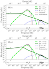 |
Fig. 1. Best fit with residuals of the multi-wavelength flux density of the 2013 observations of A0620−00 from Dinçer et al. (2017). In the upper panel, we show the result for the case of BHJet, and in the lower panel, we show the case of MLJet. The solid black line shows the total absorbed emission, and the individual components are explained in the legend. |
In Fig. 2, we show the extended energy spectrum with the radio-to-X-ray data and the sensitivity curves of three instruments in the high-energy regime. We used the sensitivity curve of INTEGRAL/SPI, the Fermi/LAT sensitivity, and the predicted Cherenkov Telescope Array Observatory CTAO sensitivity for the south site. The upper panel shows the case of BHJet, and the lower panel shows the case of MLJet. The contribution from the secondary particles and the individual components is as shown in the legend.
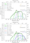 |
Fig. 2. Multi-wavelength spectrum of A0620−00 for the case of the BHJet model in the upper panel and for the case of the MLJet model in the lower panel. The solid black line shows the total emitted spectrum, and the individual components are explained in the legends. The radio-to-X-ray data are the same as in Fig. 1. We include the INTEGRAL/SPI, Fermi/LAT, and CTAO point source sensitivities for comparison. |
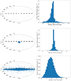 |
Fig. 3. Positions of one random realisation of qBHXBs in the sky (left) in Galactic coordinates and the histogram of their distances (right). From top to bottom, we plot the 103 sources at the GC, the 104 boxy bulge, and the 1.2 × 10⁴ Galactic disc. |
4. Multi-wavelength emission of qBHXBs
4.1. Population model
The simultaneous radio to X-ray observations of binary systems have led to the identification of about 50 BHXBs (Corral-Santana et al. 2016; Tetarenko et al. 2016a). The duty cycle of these sources is approximately 10%, that is, they spend most of their lifetime in quiescence. Following the work of Olejak et al. (2020), we extracted information about a recent population synthesis analysis. More precisely, we separately studied three different regions of the Milky Way: a Lorimer-like population of qBHXB in the Galactic disc (Lorimer et al. 2006), a further population in the boxy bulge, and a third distribution up to a few dozen parsec around the Galactic centre (GC). As the absolute size of each population, we adopted the following numbers: 103 sources in the GC, 104 in the boxy bulge, and an upper limit of 1.2 × 10⁵ sources in the disc (Olejak et al. 2020 and see discussion below). We drew random values in a 3D grid to place the sources in the three different Galactic regions, namely, we adopted a Gaussian distribution for the radial distances of the GC sources with a mean value of 2 pc and a standard deviation of 20 pc (Mori et al. 2021). For the boxy bulge, we followed the formula of Cao et al. (2013), and for the disc sources, we adopted the Lorimer distribution of Lorimer et al. (2006). We assumed that the Galactic disc is a 2D structure with a radius of 20 kpc and a height of 2 kpc above and below the Galactic plane, and the location of the Solar System at 8.3 kpc from the GC. In Fig. 3, we show the sky map and overplot the distances of the sources of each individual population with the GC, the boxy bulge in the middle, and the Lorimer-like population in the lower panels. In the left panels, we show the sky maps in Galactic coordinates, and on the right, we plot the histograms of the distances of the produced qBHXBs from the Sun.
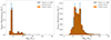 |
Fig. 4. Histogram of the masses of the BH of the qBHXBs. The shaded grey region is adopted from Olejak et al. (2020), from which we derive the Gaussian kernel shown by the solid line. The shaded orange histogram corresponds to 104 boxy bulge qBHXBs (left panel) and 1.2 × 10⁵ disc qBHXBs (right panel) used in this work. |
In addition to the spatial positions, we also modelled the BH mass distribution. Olejak et al. (2020) presented the distribution of the mass of the BH in binaries for the Galactic disc and the Galactic halo. In Fig. 4, we plot the histogram based on the supplementary material of Olejak et al. (2020), for which we find a Gaussian kernel to use as probability function distribution (PDF). From this calculated PDF, we extracted 104 and 1.2 × 10⁵ random values of the mass of the BH for the boxy bulge and the Lorimer-like distribution, respectively. We overplot the extracted random values as an orange-shaded histogram on the resulting distribution of Olejak et al. (2020).
A further important parameter of the qBHXBs is the viewing angle, that is, the angle between the jet axis and the line of sight. We lack robust constraints and therefore used a uniform PDF between 1° and 90° to evaluate the viewing angle of each qBHXB.
For each unique source, we assumed a set of parameters with the mass of the BH, the viewing angle, and the distance. Assuming that all qBHXBs behave similarly to A0620−00, we used these three quantities to rescale the emitted spectrum.
4.2. Multi-wavelength prompt emission
In Figs. 5–8, we plot the cumulative emission of all these qBHXBs in different energy bands from keV X rays to TeV γ rays. More precisely, we used the detected diffuse emission from the following instruments to investigate the contribution of qBHXBs: NuSTAR in the keV band, INTEGRAL in the ∼MeV X rays, Fermi/LAT in the GeV γ rays, and H.E.S.S., the High-Altitude Water Cherenkov Observatory (HAWC), LHAASO, and CTAO for TeV γ rays. Moreover, we compared individual sources to the instrument sensitivity to discuss their potential detection.
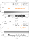 |
Fig. 5. Contribution of the prompt emission of the Galactic qBHXBs to the NuSTAR diffuse emission for 1° ≤(l, b)≤3° (Perez et al. 2019). The upper panel shows the assumed model BHJet, and the lower panel shows the MLJet. In both panels, we show the lower and upper limit of the Lorimer-like distribution (1.2 × 10⁴ versus 1.2 × 10⁵ qBHXBs) and the 103 boxy bulge-like sources based on Olejak et al. (2020). The sum of the boxy bulge and the Lorimer-like distribution leads to the total contribution, which we plot with the thin solid line for the upper limit and the thick solid line for the lower limit. The shaded grey region corresponds to the predicted contribution of these qBHXBs to the observed diffuse emission. The insets in both panels show the percentage contribution per energy bin. |
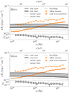 |
Fig. 6. Similar to Fig. 5, but for the energy band covered by INTEGRAL for (|l|,|b|) ≤ (47.5° ,47.5° ) (Berteaud et al. 2022). We overplot the point source sensitivity of INTEGRAL/SPI on the diffuse emission, as indicated in the legend (Roques et al. 2003), and compare it to individual sources that contribute to the total emission (solid coloured lines for individual sources). We show only sources that lie above the instrument sensitivity. No sources lie above the threshold for MLJet. |
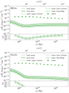 |
Fig. 7. Similar to Fig. 5, but for the energy band covered by Fermi/LAT, and only for the region around the GC with |l|≤80° and |b|≤8°. |
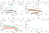 |
Fig. 8. Similar to Fig. 5, but for the highest-energy regime of TeV compared to the H.E.S.S. (top left), HAWC (top right), LHAASO (bottom left), and CTAO (bottom right) facilities. For H.E.S.S., HAWC, and LHAASO, we show with solid coloured lines the individual sources that exceed 10−3 of the point source sensitivity, and for CTAO, we show the sources that exceed one-third of the predicted point source sensitivity. For all panels, we only show the case of BHJet because the contribution of sources that follow MLJet is even smaller than pictured here. The inner (outer) region for the case of HAWC is 43° ≤l ≤ 73° and |b|≤2° (|b|≤4°), and the inner (outer) region for the case of LHAASO is 15° ≤l ≤ 125° (125° ≤l ≤ 235°) and |b|≤5°. For CTAO, the sources lie within |l|≤60° and |b|≤3° (Eckner et al. 2023). All the panels have the same axes for comparison. |
We used the NuSTAR Galactic diffuse emission from Perez et al. (2019) for a region of 3° around the GC. For the case of INTEGRAL, we adopted the analysis of Berteaud et al. (2022) for |l|≤47.5° and |b|≤47.5° for the diffuse emission and the sensitivity from Roques et al. (2003). The Fermi/LAT data for different regions in the sky map were taken from Ackermann et al. (2012) for four different regions: the Galactic disc with |l|≤80° and |b|≤8°, the intermediate disc for |l|≤180° and 10° ≤|b|≤20°, the ridge with 80° ≤|l|≤180° and |b|≤8°, and the off-plane region with |l|≤180° and 8° ≤|b|≤90°. The H.E.S.S. diffuse emission was taken from H.E.S.S. Collaboration (2018) for a region of |l|≤1° and |b|≤5°. The best fit of the HAWC Galactic diffuse emission for 43° ≤l ≤ 73° and two regions on the sky map with |b|≤2° for the innermost one, and |b|≤4° for the outermost one, are  and
and  in units of 10−12 TeV−1 s−1 cm−2 sr−1, respectively (Alfaro et al. 2024). We fixed a probable typo in the provided units. The HAWC sensitivity after 507 days was derived from Abeysekara et al. (2017). For the ∼PeV regime and the LHAASO collaboration, there are two sky map regions with |b|≤5°, the innermost map with 15° ≤l ≤ 125° and the outermost map with 125° ≤l ≤ 235° (Cao et al. 2023). Finally, we adopted the CTAO simulated sensitivity for |l|≤60° and |b|≤3° from Eckner et al. (2023). For each different energy regime, we only used sources that lay within the aforementioned regions to calculate the cumulative emission.
In Fig. 5, we show the predicted cumulative emission of the Lorimer distribution and the boxy bulge in the keV spectrum. For simplicity, we neglected the GC because it almost does not contribute at all. In the upper panel, we show the cumulative emission assuming that all the qBHXBs obey the BHJet model, and in the lower panel, we show the MLJet. As described above, the 1.2 × 10⁵ sources of Olejak et al. (2020) host a BH with a non-degenerate companion, but not necessarily all of these BHs accrete matter from the companion at the same time. We therefore used this value as an upper limit (the densely dotted line labelled ‘Lorimer upper’), and we combined it with a lower limit assuming that 10% of these sources accrete at a time (see the more detailed discussion below). Summing the boxy bulge with either the upper or lower limit of the Lorimer yields the total emission in the keV X-ray band between some upper and some lower limits (total upper and total lower, respectively). The shaded grey region therefore shows the total predicted emission from the Galactic qBHXBs between the upper limit of the Lorimer and some lower case of 10%. In the insets of the upper and lower panels, we show the percentage of the potential contribution of the qBHXBs to the NuSTAR diffuse emission. For both jet models and depending on the number of disc sources, the contribution might be of about a few to 20%.
In Fig. 6, we plot the contribution of the qBHXBs to the INTEGRAL diffuse emission (orange crosses) following the above pattern. The contribution of qBHXBs to this energy band is larger; it reaches values of almost 100% in the ∼100 keV to a few percent in the regions of dozens of MeV. In the same plots, we include the sensitivity of INTEGRAL/SPI for point sources from Roques et al. (2003) to compare to individual sources. For the case of BHJet, we find that a few sources might exceed the sensitivity in the first several energy bins in the ∼40−100 keV.
In Fig. 7, we plot the predicted contribution of qBHXBs to the GeV γ rays compared to the Fermi/LAT detection of the extended region around the GC. We again used the same pattern as above to derive the upper limit of the total emission assuming an upper limit for the Lorimer-like disc distribution, and a smaller fraction of this at 10%. The overall contribution drops to less than 0.1% in these energy bins, and for the case of the BHJet, the contribution drops below 10−4% at energies beyond GeV. For MLJet on the other hand, the contribution can reach about 0.1% not only in the GeV energies, but also in the 100 GeV. In Appendix A, we show the predicted contribution of qBHXBs at intermediate Galactic latitudes, the ridge and the off plane for BHJet and MLJet. We see no more than 0.1% in the 1 GeV and 100 GeV energy bins, similar to the GC.
Finally, in Fig. 8 we combine the three operating TeV facilities of H.E.S.S., HAWC, and LHAASO with the under-construction next-generation facility of CTAO. qBHXBs can contribute up to 0.5% of the 1−10 TeV diffuse emission detected by H.E.S.S., but no individual sources are expected to be detected by H.E.S.S. (no individual sources exceed the plotted sensitivity). The qBHXBs of the ridge, that is, only sources from the disc, can contribute up to 0.3% in the TeV diffuse emission detected by HAWC, and up to 0.1% in the 10 TeV emission detected by LHAASO. For LHAASO, and the outer region, in particular, where 125° ≤l ≤ 235°, the contribution drops as a function of energy and falls below 10−4%. Finally, in Fig. 8, we compare some individual sources that we find that may produce significant TeV emission close to 10−13 erg s−1 cm−2 with the predicted CTAO sensitivity for point source detection in the Galactic plane. In Fig. 8, we only include the predicted emission from qBHXBs using the BHJet jet model because the case of MLJet yields some TeV emission that is significantly lower, and the overall contribution therefore drops significantly to even lower than 10−4%. We adopted this threshold here.
4.3. Cosmic-ray fluxes and multi-wavelength secondary emission
We have only accounted for the intrinsic emission from the jets of qBHXBs for either BHJet or MLJet above. This intrinsic radiation is the product of the non-thermal CRs that are accelerated within the jets. When these CRs, or more precisely, a fraction of these CRs, escape from the acceleration sites, they propagate in the Milky Way. Using numerical means to follow this propagation, we estimated the CR flux detected here on Earth, and we compared it to the detected spectrum. In particular, we used DRAGON2, a publicly available simulator of the Galactic propagation. We assumed that the CR sources are the same as above, namely a Gaussian population around the GC, a boxy bulge, and a Lorimer-like disc distribution. The normalisation of each distribution is thoroughly explained in Appendix B. Each qBHXB ejects some CRs in the Milky Way that follow a power law in energies similar to the intrinsic power law, and they carry some total power that we show in Table 2. Moreover, we calculated the maximum of the CR energy to be about 20 TeV (see Table 2). As we show in Appendix C, the contribution of the propagated protons is smaller than 10−10, and it is about 10−12 for electrons.
Calculated power carried by the non-thermal protons (p) and electrons (e) and their maximum energy for the two jet models.
5. Discussion
5.1. BHJet vs MLJet for A0620–00
To finally determine the exact number of qBHXBs in the Milky Way and their role in the multi-wavelength emission, we need to investigate the physics of individual sources better, such as A0620−00. With the BHJet and MLJet jet models, we captured the broadband electromagnetic picture from radio to X-rays. More precisely, the thermal synchrotron emission from the jet base can explain the IR emission along with the stellar emission of the companion, in agreement with Dinçer et al. (2017). The synchrotron optically thick emission connects the radio to the X-ray emission, similar to various BHXBs in outburst (Merloni et al. 2003; Falcke et al. 2004; Plotkin et al. 2014). In both cases, however, the IC contributes equally, and it is therefore impossible to distinguish the two components with a spectral fitting alone. Further means are needed, such as a timing analysis. Nonetheless, we were able to constrain the jet dynamics to predict the hard X-ray and γ-ray emission. In both scenarios and assuming an efficient particle acceleration, the optically thick synchrotron emission reaches the MeV bands that emerge from a cooled population of non-thermal electrons. The distribution of these electrons is the convolution of a thermal Maxwell-Jüttner and a non-thermal tail that expands to energies of about 10 TeV (see Table 2) for a power-law index close to 2 (see Table 1). This distribution is similar to the one plotted in Fig. 6 of K22, but for a softer index. The radiation footprint of this leptonic population to dozens of TeV energies is the flat spectrum in the keV–MeV regime in a νFν(ν) plot (see the Syn, z > zdiss component of Fig. 2). This sub-MeV emission is hard to detect with either INTEGRAL or Fermi/LAT under these jet conditions.
The main differences between the two jet models are in the GeV and beyond spectrum and in the jet composition. Starting from the latter, for BHJet we assumed an equal number density of electrons and protons all along the jet. For MLJet, on the other hand, as we describe in Sect. 2, the jets are launched with η pairs of electrons and positrons with respect to pairs of electrons and protons. For A0620−00, we used this as a free parameter, and we found that ∼200 pairs per proton are needed to explain the radio to X-ray emission. This difference in the jet composition leads to different spectral components in the TeV band. In particular, the neutral pion decay from pp interactions is reduced in the case of MLJet because fewer targets reside in the jets that allow for an inelastic collision, but more target electrons exist, which enable a stronger IC component (stronger than BHJet, but still not strong enough to increase the GeV flux significantly). This more physically motivated proton power allows for better constraints in terms of jet energetics, but unfortunately, it does not lead to stronger non-thermal γ-ray emission.
5.2. Population of BHXBs in the disc
According to Olejak et al. (2020), 1.2 × 10⁵ qBHXBs may reside in the Galactic disc, but this number is very uncertain. However, only a fraction of these sources are currently expected to accrete and launch jets simultaneously. Based on the radio detection of another qBHXB, namely VLA J2130+12, Tetarenko et al. (2016b) estimated that 2.6 × 10⁴ − 1.7 × 10⁸ objects may exist in the Milky Way at the moment. The lower limit is of the same order of magnitude as the value we used as a lower limit of the current qBHXBs (for simplicity, we used 1.2 × 10⁴ sources, that is, 10% of the total population). This number of qBHXBs might agree with the more recent observations of Gaia, which detected approximately 6 × 10³ ellipsoidal systems, a few percent of which harbour a compact object (Gomel et al. 2023). Gaia detected only nearby binaries, however, and only those with an orbital period shorter than a few days can be claimed to be binaries.
The estimated lower limit of Tetarenko et al. (2016b) is consistent with the upper limit of theoretical predictions for the number of BHXBs in the Milky Way based on population synthesis (see e.g. Romani 1992; Portegies Zwart et al. 1997; Kalogera & Webbink 1998; Pfahl et al. 2003; Yungelson et al. 2006; Kiel & Hurley 2006). Nonetheless, in the population synthesis studies, the fraction of accreting BHXBs is typically ∼0.01% within a Hubble time (Yungelson et al. 2006). The more recent analysis by Wiktorowicz et al. (2019) showed that ∼104 BHXBs are expected to fill their Roche lobe. This value is only 1% of the total population of sources.
The estimated upper limit of Tetarenko et al. (2016b) is approximately two orders of magnitude above the upper limit we used. Figs. 5 and 6 showed that the X-ray diffuse emission does not allow for more than 105 jetted qBHXBs at the same time. A further comparison, however, might not lead to concrete conclusions because our main assumption that all these 1.2 × 10⁴ − 1.2 × 10⁵ qBHXBs launch jets of approximately the same power cannot rule out the existence of even more qBHXBs that lack any jet emission. Consequently, it is worthwhile to revisit the contradiction between the theoretical prediction of ≤104 and the observational evidence for ≥104 so that we can better constrain the contribution of (q)BHXBs to the observed diffuse Galactic radio to γ-ray emission detected, and vice versa, the further observational investigation of (q)BHXBs can help us to better constrain the contribution of these sources to the Galactic diffuse emission.
5.3. X-ray to γ-ray contribution to the diffuse emission
The diffuse X-ray emission detected by NuSTAR is mainly up to 90% due to cataclysmic variables (Perez et al. 2019). Some 10% of this emission, however, is due to unresolved Galactic sources. We found that qBHXBs that launch jets can contribute up to 10% depending on the jet model. The contribution can be reduced to a few percent because the number of accreting qBHXBs drops to 10%, that is, about 1.2 × 10⁴ sources in the Galactic disc.
In the more energetic X-ray regime, and in particular, in the energy window observed by INTEGRAL, we find that the qBHXBs can fully explain the ∼100 keV band and up to a few percent to the regime of some dozen keV. It is worth mentioning that in the X-ray analysis of the INTEGRAL data, the contribution of the unresolved sources is commonly assumed to follow a power law in energy with an exponential cutoff (see, e.g. Berteaud et al. 2022), but based on this analysis, the contribution of qBHXBs is energy dependent and decreases with energy. This energy dependence of the contribution is due to radiatively cooled electrons that are accelerated in the qBHXBs jets. For a less efficient particle acceleration in which the particles escape from the acceleration sites long before they reach their theoretical maximum energy, the X-ray spectrum would show a cutoff at much lower energies than some dozen MeV, but still in the X-ray band. The contribution of qBHXBs to the high-energy tail may hence drop, unlike in the lower regime at 100 keV.
When we compare the INTEGRAL sensitivity for individual sources to the predicted emission of some individual qBHXBs that contribute the most to the diffuse emission in the softer regime of the MeV X-ray spectrum, we expect one source at most to be detected in the 30−100 keV regime for the case of BHJet. For a more accurate prediction of this value, we performed 250 realisations of our simulations to find out that 0.4 ± 0.5 sources are expected to be detected by INTEGRAL on average. This value indeed agrees well with the number of BHXBs detected by INTEGRAL so far, but no qBHXB has been detected to date.
In the higher-energy regime of γ rays, the contribution of qBHXBs is smaller than 1% in the entire spectrum from GeV to TeV energies. The CTAO, however, is expected to be ten times more sensitive than current facilities. To predict numbers more reliably for this energy regime, we realised 250 simulations, according to which, 1 ± 0.5 sources are expected to be detected by CTAO. It is worth remarking that these sources are merely in the quiescence and not during outburst, when stronger TeV emission is expected (see e.g. Kantzas et al. 2023a). For these sources that exceed the CTAO sensitivity in each realisation of the simulations, the CTAO will be able to detect sources that are located closer than ∼2 kpc (with an average distance of 0.9 ± 0.4 kpc) and have a viewing angle smaller than 17° (with an average viewing angle of 11 ± 2°). The majority of the BHXBs known so far are beyond 1 kpc, and the nearest system lies at 0.5 kpc (El-Badry et al. 2022; Chakrabarti et al. 2023). Only the viewing angle of MAXI J1836–194 is smaller than 15° and located farther away than 4 kpc (Russell et al. 2014). We obtained these results under the assumption that all qBHXBs follow the spectral behaviour of A0620−00 because the number of qBHXBs with good-quality multi-wavelength data is still small. If CTAO can indeed detect TeV emission from individual qBHXBs, this will allow us to study a new part of the parameter space.
5.4. Radio counterparts and predictions for future facilities
The radio counterpart of qBHXBs, such as the one detected by the VLA from A0620−00 (Dinçer et al. 2017), is a key element to prove the jet emission, particularly in the case of a flat radio spectrum (Blandford & Königl 1979). Current facilities such as the VLA and MeerKAT can detect sources with a radio intensity lower than 100 μJy and can sometimes reach values close to 10 μJy (Driessen et al. 2019; Goedhart et al. 2024). In the future, with ngVLA (Butler et al. 2019) and the full array of the SKA (Braun et al. 2017), the threshold for a detection may drop to ∼ μJy. In Fig. 9, we plot the cumulative distribution of sources per energy flux at 1.28 GHz. The two different histograms correspond to the assumption of the upper/lower Lorimer distribution, similar to what we described above. For the current threshold of ∼10 μJy, we may be able to detect up to a few hundred sources, depending on the number of jetted qBHXBs (lower and upper limits, respectively). Simultaneous multi-wavelength observations in the optical and/or the X-rays, as well as a timing analysis that indicates periodicity, are necessary to identify these radio sources as (q)BHXBs (see e.g. Driessen et al. 2019).
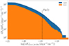 |
Fig. 9. Cumulative distribution of sources per energy flux detected at a characteristic radio frequency of 1.28 GHz. The two histograms correspond to the two assumptions for an upper or lower limit of qBHXBs populating a Lorimer-like distribution in the disc. We show for comparison the detection threshold of radio sources with current facilities, such as MeerKAT and VLA (∼10 μJy). |
5.5. Neutrino counterpart
The recent Galactic neutrino diffuse emission detected by IceCube strengthens the idea that non-thermal accelerators exist in the Galactic plane (IceCube Collaboration 2023). The hadronic processes that can take place in the jets of BHXBs lead to the formation of non-thermal astrophysical neutrinos that reach energies of about a few dozen TeV. To determine the possible contribution of the qBHXBs to the detected Galactic neutrinos, we self-consistently estimated the neutrino emission from each individual source for all the three source populations. In Fig. 10, we plot the total neutrino flux expected from the qBHXBs in the Milky Way, and we compare it to the detected Galactic diffuse emission. More precisely, the detected neutrino spectrum depends on the model, and for three different CR propagation models, IceCube Collaboration (2023) derived three different neutrino spectra. The π0 corresponds to the CR propagation model of Galprop, which uses as a normalisation the Fermi/LAT observations of the diffuse γ-ray emission (Ackermann et al. 2012), whereas the KRAγ model corresponds to the CR propagation, for which the diffusion coefficient is spatially dependent, and there is an exponential cutoff in the propagating CR power-law at 5 or 50 PeV (KRAγ5 and KRA , respectively; Gaggero et al. 2015).
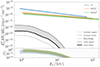 |
Fig. 10. Predicted neutrino flux from the source populations as shown in the legend (also see Fig. 5), assuming that the BHJet jet scenario explains their jet dynamics. The subplot shows the contribution of the total predicted flux to the detected Galactic neutrino diffuse emission by IceCube (IceCube Collaboration 2023). The three different colours represent the three different models used to extract the observed flux. |
We only show the case of BHJet because neutrino emission in the MLJet scenario is further suppressed (see the discussion above for γ rays). The total contribution of qBHXBs to the detected spectrum is smaller than 1% at an energy of about 1−2 TeV, which rapidly drops to even less than 10−2% at an energy of about 10 TeV.
6. Summary and conclusions
BHXBs have recently been suggested as Galactic CR sources (Romero et al. 2003; Romero & Orellana 2005; Torres et al. 2005; Bednarek et al. 2005; Reynoso et al. 2008; Cooper et al. 2020; Carulli et al. 2021; Kantzas et al. 2023b). Most of these objects spend their lifetimes in quiescence, and only a handful of these are detected from the radio to X-rays. Recent observations of qBHXBs suggest the existence of relativistic jets that can accelerate particles to high energies. We examined this scenario based on the well-studied qBHXB A0620−00. We used in particular two different jet models, BHJet and MLJet, and we found that both explain the radio-to-X-ray electromagnetic spectrum well. Non-thermal relativistic electrons may reach energies of some dozen TeV that lead to some strong synchrotron and IC emission, which can explain the X-ray spectrum. Regardless of the acceleration of protons to non-thermal energies, we find that no significant γ-ray radiation from this source is produced that could be detected by current or planned facilities.
The exact number of BHXBs and qBHXBs is debated. Observations and simulations yield values that range between a few thousand to up to 108. Following the population synthesis analysis of Olejak et al. (2020), we examined the contribution of 1.2 × 10⁴ − 1.2 × 10⁵ qBHXBs to the CR spectrum and the X-ray/γ-ray Galactic diffuse emission. While no significant contribution is expected in either the electron or proton CR spectra detected on Earth, we find that the cumulative intrinsic emission of these objects can contribute significantly to the Galactic diffuse emission. More precisely, assuming that all the qBHXBs have the same spectral behaviour as A0620−00 but rescaled for the distance and viewing angle, we derived the predicted spectrum from X-rays to γ rays. For a population of 104 sources located in the boxy bulge and between 1.2 × 10⁴ − 1.2 × 10⁵ in the Galactic disc, qBHXBs can explain up to 10% of the keV X-ray spectrum, depending on the jet conditions. This is the highest possible contribution, and more conservative numbers of qBHXBs can reduce the contribution to a few percent. The soft MeV Galactic diffuse emission is expected to be dominated by cataclysmic variables and IC of CR electrons, but qBHXBs can contribute up to 10−90%, depending on the jet dynamics and the exact number of sources. We find, moreover, that the contribution of qBHXBs to the unresolved hard MeV spectrum decreases with energy because the emission originates in the non-thermal synchrotron emission of radiatively cooled electrons. This feature may help us to identify the origin of the MeV diffuse emission better. The radio counterpart of qBHXBs may reveal their exact number. Current radio facilities that are sensitive to ∼10 μJy, such as MeerKAT, could detect some dozen qBHXBs that can constrain their absolute number in the Milky Way better. In the more energetic regime, CTAO will detect some of these sources, in particular, those that reside at distances shorter than 2 kpc and with viewing angles smaller than 15° to allow for further boosting. These sources have only recently become detectable at distances as close as 0.5 kpc and with viewing angles as low as ∼10°, and further observations would therefore help us to better constrain the contribution of BHXBs and qBHXBs in particular to the CR spectrum and the Galactic diffuse emission. Finally, qBHXBs may explain up to 1% of the diffuse neutrino background as detected by IceCube. Their contribution decreases significantly at neutrino energies beyond ∼10 TeV.
One gravitational radius is defined as rg = GMbh/c2 ≃ 1.5 × 10⁵ (Mbh/M⊙) cm, where G is the gravitational constant, Mbh is the mass of the black hole, c is the speed of light, and M⊙ is the solar mass.
Acknowledgments
We are grateful for the very fruitful comments of the anonymous reviewer. DK and FC acknowledge funding from the French Programme d’investissements d’avenir through the Enigmass Labex, and from the ‘Agence Nationale de la Recherche’, grant number ANR-19-CE310005-01 (PI: F. Calore). We thank Thomas Siegert for useful discussions on the INTEGRAL/SPI analysis, and Marco Chianese on the non-thermal processes.
References
- Abeysekara, A., Albert, A., Alfaro, R., et al. 2017, ApJ, 843, 39 [NASA ADS] [CrossRef] [Google Scholar]
- Abeysekara, A., Albert, A., Alfaro, R., et al. 2018, Nature, 562, 82 [CrossRef] [Google Scholar]
- Ackermann, M., Ajello, M., Atwood, W. B., et al. 2012, ApJ, 750, 3 [NASA ADS] [CrossRef] [Google Scholar]
- Aguilar, M., Aisa, D., Alvino, A., et al. 2014, Phys. Rev. Lett., 113, 121102 [Google Scholar]
- Aguilar, M., Aisa, D., Alpat, B., et al. 2015, Phys. Rev. Lett., 114, 171103 [CrossRef] [PubMed] [Google Scholar]
- Alfaro, R., Alvarez, C., Arteaga-Velázquez, J. C., et al. 2024, ApJ, 961, 104 [NASA ADS] [CrossRef] [Google Scholar]
- Amenomori, M., Bao, Y. W., Bi, X. J., et al. 2021, Phys. Rev. Lett., 126, 141101 [NASA ADS] [CrossRef] [Google Scholar]
- Apel, W. D., Arteaga-Velázquez, J. C., Bekk, K., et al. 2011, Phys. Rev. Lett., 107, 171104 [CrossRef] [PubMed] [Google Scholar]
- Baade, W., & Zwicky, F. 1934, Proc. Natl. Acad. Sci., 20, 259 [NASA ADS] [CrossRef] [Google Scholar]
- Bednarek, W., Burgio, G., & Montaruli, T. 2005, New Astron. Rev., 49, 1 [CrossRef] [Google Scholar]
- Berteaud, J., Calore, F., Iguaz, J., Serpico, P., & Siegert, T. 2022, Phys. Rev. D, 106, 023030 [CrossRef] [Google Scholar]
- Blandford, R., & Königl, A. 1979, ApJ, 232, 34 [NASA ADS] [CrossRef] [Google Scholar]
- Blandford, R. D., & Payne, D. G. 1982, MNRAS, 199, 883 [CrossRef] [Google Scholar]
- Blandford, R. D., & Znajek, R. L. 1977, MNRAS, 179, 433 [NASA ADS] [CrossRef] [Google Scholar]
- Blasi, P. 2013, A&ARv, 21, 70 [Google Scholar]
- Böttcher, M., Reimer, A., Sweeney, K., & Prakash, A. 2013, ApJ, 768, 54 [Google Scholar]
- Braun, R., Bonaldi, A., Bourke, T., Keane, E., & Wagg, J. 2017, SKA-TEL-SKO-0000818 [Google Scholar]
- Butler, B., Grammer, W., Selina, R., Murphy, E., & Carilli, C. 2019, ngVLA Sensitivity, Tech. rep., ngVLA Memo 21 [Google Scholar]
- Calore, F., Cholis, I., McCabe, C., & Weniger, C. 2015, Phys. Rev. D, 91, 063003 [CrossRef] [Google Scholar]
- Cangemi, F., Rodriguez, J., Grinberg, V., et al. 2021, A&A, 645, A60 [NASA ADS] [CrossRef] [EDP Sciences] [Google Scholar]
- Cantrell, A. G., Bailyn, C. D., Orosz, J. A., et al. 2010, ApJ, 710, 1127 [NASA ADS] [CrossRef] [Google Scholar]
- Cao, L., Mao, S., Nataf, D., Rattenbury, N. J., & Gould, A. 2013, MNRAS, 434, 595 [NASA ADS] [CrossRef] [Google Scholar]
- Cao, Z., Aharonian, F., Zhao, L., et al. 2023, Phys. Rev. Lett., 131, 151001 [NASA ADS] [CrossRef] [Google Scholar]
- Carulli, A. M., Reynoso, M. M., & Romero, G. E. 2021, Astropart. Phys., 128, 102557 [Google Scholar]
- Chakrabarti, S., Simon, J. D., Craig, P. A., et al. 2023, ApJ, 166, 6 [CrossRef] [Google Scholar]
- Chang, J., Adams, J., Ahn, H., et al. 2008, Nature, 456, 362 [NASA ADS] [CrossRef] [Google Scholar]
- Chatterjee, K., Liska, M., Tchekhovskoy, A., & Markoff, S. B. 2019, MNRAS, 490, 2200 [Google Scholar]
- Connors, R., Markoff, S., Nowak, M., et al. 2016, MNRAS, 466, 4121 [Google Scholar]
- Connors, R. M. T., van Eijnatten, D., Markoff, S., et al. 2019, MNRAS, 485, 3696 [CrossRef] [Google Scholar]
- Cooper, A. J., Gaggero, D., Markoff, S., & Zhang, S. 2020, MNRAS, 493, 3212 [Google Scholar]
- Corbel, S., & Fender, R. P. 2002, ApJ, 573, L35 [NASA ADS] [CrossRef] [Google Scholar]
- Corbel, S., Fender, R. P., Tzioumis, A. K., et al. 2000, A&A, 359, 251 [NASA ADS] [Google Scholar]
- Corbel, S., Coriat, M., Brocksopp, C., et al. 2012, MNRAS, 428, 2500 [Google Scholar]
- Corral-Santana, J. M., Casares, J., Muñoz-Darias, T., et al. 2016, A&A, 587, A61 [NASA ADS] [CrossRef] [EDP Sciences] [Google Scholar]
- DAMPE Collaboration (An, Q., et al.) 2019, Sci. Adv., 5, eaax3793 [NASA ADS] [CrossRef] [Google Scholar]
- dePolo, D. L., Plotkin, R. M., Miller-Jones, J. C. A., et al. 2022, MNRAS, 516, 4640 [NASA ADS] [CrossRef] [Google Scholar]
- Dinçer, T., Bailyn, C. D., Miller-Jones, J. C., Buxton, M., & MacDonald, R. K. 2017, ApJ, 852, 4 [Google Scholar]
- Dodelson, S., Hooper, D., & Serpico, P. D. 2008, Phys. Rev. D, 77, 063512 [CrossRef] [Google Scholar]
- Driessen, L. N., McDonald, I., Buckley, D. A. H., et al. 2019, MNRAS, 491, 560 [Google Scholar]
- Eckner, C., Vodeb, V., Martin, P., Zaharijas, G., & Calore, F. 2023, MNRAS, 521, 3793 [NASA ADS] [CrossRef] [Google Scholar]
- El-Badry, K., Rix, H.-W., Quataert, E., et al. 2022, MNRAS, 518, 1057 [NASA ADS] [CrossRef] [Google Scholar]
- Falcke, H., & Biermann, P. L. 1994, A&A, 293, 665 [NASA ADS] [Google Scholar]
- Falcke, H., Körding, E., & Markoff, S. 2004, A&A, 414, 895 [NASA ADS] [CrossRef] [EDP Sciences] [Google Scholar]
- Fender, R. P. 2001, MNRAS, 322, 31 [NASA ADS] [CrossRef] [Google Scholar]
- Fender, R. P., Belloni, T. M., & Gallo, E. 2004, MNRAS, 355, 1105 [NASA ADS] [CrossRef] [Google Scholar]
- Fender, R. P., Maccarone, T. J., & van Kesteren, Z. 2005, MNRAS, 360, 1085 [Google Scholar]
- Fender, R. P., Homan, J., & Belloni, T. M. 2009, MNRAS, 396, 1370 [NASA ADS] [CrossRef] [Google Scholar]
- Foreman-Mackey, D., Hogg, D. W., Lang, D., & Goodman, J. 2013, PASP, 125, 306 [Google Scholar]
- Gaggero, D., Grasso, D., Marinelli, A., Urbano, A., & Valli, M. 2015, ApJ, 815, L25 [NASA ADS] [CrossRef] [Google Scholar]
- Gallo, E., Fender, R., Kaiser, C., et al. 2005, Nature, 436, 819 [Google Scholar]
- Gallo, E., Migliari, S., Markoff, S., et al. 2007, ApJ, 670, 600 [NASA ADS] [CrossRef] [Google Scholar]
- Gallo, E., Miller-Jones, J. C. A., Russell, D. M., et al. 2014, MNRAS, 445, 290 [CrossRef] [Google Scholar]
- Gandhi, P., Blain, A. W., Russell, D. M., et al. 2011, ApJ, 740, L13 [NASA ADS] [CrossRef] [Google Scholar]
- Ginzburg, V. L., & Syrovatskii, S. I. 1964, The Origin of Cosmic Rays (Elsevier) [Google Scholar]
- Goedhart, S., Cotton, W. D., Camilo, F., et al. 2024, MNRAS, 531, 649 [CrossRef] [Google Scholar]
- Gomel, R., Mazeh, T., Faigler, S., et al. 2023, A&A, 674, A19 [NASA ADS] [CrossRef] [EDP Sciences] [Google Scholar]
- H.E.S.S. Collaboration (Abdalla, H., et al.) 2018, A&A, 612, A9 [NASA ADS] [CrossRef] [EDP Sciences] [Google Scholar]
- Hillas, A. M. 1984, ARA&A, 22, 425 [Google Scholar]
- Houck, J. C., & Denicola, L. A. 2000, ASP Conf. Ser., 216, 591 [Google Scholar]
- IceCube Collaboration (Abbasi, R., et al.) 2023, Science, 380, 1338 [NASA ADS] [CrossRef] [Google Scholar]
- Janssen, M., Falcke, H., Kadler, M., et al. 2021, Nat. Astron., 5, 1017 [NASA ADS] [CrossRef] [Google Scholar]
- Jokipii, J. 1987, ApJ, 313, 842 [NASA ADS] [CrossRef] [Google Scholar]
- Kalogera, V., & Webbink, R. F. 1998, ApJ, 493, 351 [NASA ADS] [CrossRef] [Google Scholar]
- Kantzas, D., Markoff, S., Beuchert, T., et al. 2021, MNRAS, 500, 2112 [Google Scholar]
- Kantzas, D., Markoff, S., Lucchini, M., et al. 2022, MNRAS, 510, 5187 [NASA ADS] [CrossRef] [Google Scholar]
- Kantzas, D., Markoff, S., Lucchini, M., Ceccobello, C., & Chatterjee, K. 2023a, MNRAS, 520, 6017 [NASA ADS] [CrossRef] [Google Scholar]
- Kantzas, D., Markoff, S., Cooper, A. J., et al. 2023b, MNRAS, 524, 1326 [NASA ADS] [CrossRef] [Google Scholar]
- Keivani, A., Murase, K., Petropoulou, M., et al. 2018, ApJ, 864, 84 [Google Scholar]
- Kelner, S., & Aharonian, F. 2008, Phys. Rev. D, 78, 034013 [CrossRef] [Google Scholar]
- Kelner, S., Aharonian, F. A., & Bugayov, V. 2006, Phys. Rev. D, 74, 034018 [NASA ADS] [CrossRef] [Google Scholar]
- Kiel, P. D., & Hurley, J. R. 2006, MNRAS, 369, 1152 [NASA ADS] [CrossRef] [Google Scholar]
- Koljonen, K. I., Hannikainen, D. C., McCollough, M., Pooley, G., & Trushkin, S. 2010, MNRAS, 406, 307 [NASA ADS] [CrossRef] [Google Scholar]
- Korol, V., Rossi, E. M., & Barausse, E. 2018, MNRAS, 483, 5518 [Google Scholar]
- Liodakis, I., & Petropoulou, M. 2020, ApJ, 893, L20 [Google Scholar]
- Lorimer, D. R., Faulkner, A. J., Lyne, A. G., et al. 2006, MNRAS, 372, 777 [NASA ADS] [CrossRef] [Google Scholar]
- Lucchini, M., Markoff, S., Crumley, P., Krauß, F., & Connors, R. M. T. 2018, MNRAS, 482, 4798 [Google Scholar]
- Lucchini, M., Krauss, F., & Markoff, S. 2019, MNRAS, 489, 1633 [NASA ADS] [Google Scholar]
- Lucchini, M., Russell, T. D., Markoff, S. B., et al. 2021, MNRAS, 501, 5910 [NASA ADS] [CrossRef] [Google Scholar]
- Lucchini, M., Ceccobello, C., Markoff, S., et al. 2022, MNRAS, 517, 5853 [NASA ADS] [CrossRef] [Google Scholar]
- Maitra, D., Markoff, S., Brocksopp, C., et al. 2009, MNRAS, 398, 1638 [NASA ADS] [CrossRef] [Google Scholar]
- Mannheim, K. 1993, A&A, 269, 67 [NASA ADS] [Google Scholar]
- Mannheim, K., & Schlickeiser, R. 1994, A&A, 286, 983 [NASA ADS] [Google Scholar]
- Markoff, S., Falcke, H., & Fender, R. 2001, A&A, 372, L25 [NASA ADS] [CrossRef] [EDP Sciences] [Google Scholar]
- Markoff, S., Nowak, M., Corbel, S., Fender, R., & Falcke, H. 2003, A&A, 397, 645 [CrossRef] [EDP Sciences] [Google Scholar]
- Markoff, S., Nowak, M. A., & Wilms, J. 2005, ApJ, 635, 1203 [NASA ADS] [CrossRef] [Google Scholar]
- Markoff, S., Nowak, M. A., Gallo, E., et al. 2015, ApJ, 812, L25 [NASA ADS] [CrossRef] [Google Scholar]
- Marscher, A. P., Jorstad, S. G., D’Arcangelo, F. D., et al. 2008, Nature, 452, 966 [Google Scholar]
- Mastichiadis, A., & Kirk, J. G. 2002, PASA, 19, 138 [CrossRef] [Google Scholar]
- McClintock, J., Remillard, R., Lewin, W., & Van Der Klis, M. 2006, in Compact Stellar X-ray Sources, eds. W. H. G. Lewin, & M. van der Klis, 71 [Google Scholar]
- Merloni, A., Heinz, S., & Di Matteo, T. 2003, MNRAS, 345, 1057 [NASA ADS] [CrossRef] [Google Scholar]
- Miller-Jones, J. C., Blundell, K. M., Rupen, M. P., et al. 2004, ApJ, 600, 368 [NASA ADS] [CrossRef] [Google Scholar]
- Mirabel, I., & Rodriguez, L. 1994, Nature, 371, 46 [NASA ADS] [CrossRef] [Google Scholar]
- Mori, K., Hailey, C. J., Schutt, T. Y. E., et al. 2021, ApJ, 921, 148 [NASA ADS] [CrossRef] [Google Scholar]
- Mücke, A., Protheroe, R., Engel, R., Rachen, J., & Stanev, T. 2003, Astropart. Phys., 18, 593 [CrossRef] [Google Scholar]
- Olejak, A., Belczynski, K., Bulik, T., & Sobolewska, M. 2020, A&A, 638, A94 [NASA ADS] [CrossRef] [EDP Sciences] [Google Scholar]
- Perez, K., Krivonos, R., & Wik, D. R. 2019, ApJ, 884, 153 [Google Scholar]
- Pfahl, E., Rappaport, S., & Podsiadlowski, P. 2003, ApJ, 597, 1036 [NASA ADS] [CrossRef] [Google Scholar]
- Plotkin, R. M., Markoff, S., Kelly, B. C., Körding, E., & Anderson, S. F. 2011, MNRAS, 419, 267 [Google Scholar]
- Plotkin, R. M., Gallo, E., & Jonker, P. G. 2013, ApJ, 773, 59 [NASA ADS] [CrossRef] [Google Scholar]
- Plotkin, R. M., Gallo, E., Markoff, S., et al. 2014, MNRAS, 446, 4098 [Google Scholar]
- Plotkin, R. M., Miller-Jones, J. C. A., Gallo, E., et al. 2017, ApJ, 834, 104 [NASA ADS] [CrossRef] [Google Scholar]
- Portegies Zwart, S. F., Verbunt, F., & Ergma, E. 1997, A&A, 321, 207 [Google Scholar]
- Rachen, J. P., & Biermann, P. L. 1993, A&A, 272, 161 [NASA ADS] [Google Scholar]
- Rachen, J. P., & Mészáros, P. 1998, Phys. Rev. D, 58, 123005 [NASA ADS] [CrossRef] [Google Scholar]
- Reynoso, M. M., Romero, G. E., & Christiansen, H. R. 2008, MNRAS, 387, 1745 [NASA ADS] [CrossRef] [Google Scholar]
- Romani, R. W. 1992, ApJ, 399, 621 [NASA ADS] [CrossRef] [Google Scholar]
- Romero, G. E., & Orellana, M. 2005, A&A, 439, 237 [NASA ADS] [CrossRef] [EDP Sciences] [Google Scholar]
- Romero, G. E., Torres, D. F., Bernadó, M. K., & Mirabel, I. 2003, A&A, 410, L1 [NASA ADS] [CrossRef] [EDP Sciences] [Google Scholar]
- Roques, J. P., Schanne, S., von Kienlin, A., et al. 2003, A&A, 411, L91 [NASA ADS] [CrossRef] [EDP Sciences] [Google Scholar]
- Russell, D. M., & Shahbaz, T. 2014, MNRAS, 438, 2083 [NASA ADS] [CrossRef] [Google Scholar]
- Russell, T. D., Soria, R., Motch, C., et al. 2014, MNRAS, 439, 1381 [CrossRef] [Google Scholar]
- Safi-Harb, S., Intyre, B. M., Zhang, S., et al. 2022, ApJ, 935, 163 [NASA ADS] [CrossRef] [Google Scholar]
- Sironi, L., Rowan, M. E., & Narayan, R. 2021, ApJ, 907, L44 [CrossRef] [Google Scholar]
- Tavani, M., Bulgarelli, A., Piano, G., et al. 2009, Nature, 462, 620 [NASA ADS] [CrossRef] [Google Scholar]
- Tavecchio, F., Maraschi, L., & Ghisellini, G. 1998, ApJ, 509, 608 [Google Scholar]
- Tetarenko, B. E., Sivakoff, G. R., Heinke, C. O., & Gladstone, J. C. 2016a, ApJS, 222, 15 [Google Scholar]
- Tetarenko, B., Bahramian, A., Arnason, R., et al. 2016b, ApJ, 825, 10 [NASA ADS] [CrossRef] [Google Scholar]
- Torres, D. F., Romero, G. E., & Mirabel, F. 2005, Chin. Astron. Astrophys., 5, 183 [CrossRef] [Google Scholar]
- Tramacere, A., Giommi, P., Perri, M., Verrecchia, F., & Tosti, G. 2009, A&A, 501, 879 [NASA ADS] [CrossRef] [EDP Sciences] [Google Scholar]
- Wiktorowicz, G., Wyrzykowski, Ł., Chruslinska, M., et al. 2019, ApJ, 885, 1 [NASA ADS] [CrossRef] [Google Scholar]
- Yoon, Y. S., Anderson, T., Barrau, A., et al. 2017, ApJ, 839, 5 [CrossRef] [Google Scholar]
- Yungelson, L., Lasota, J.-P., Nelemans, G., et al. 2006, A&A, 454, 559 [NASA ADS] [CrossRef] [EDP Sciences] [Google Scholar]
- Zanin, R., Fernández-Barral, A., de Oña Wilhelmi, E., et al. 2016, A&A, 596, A55 [NASA ADS] [CrossRef] [EDP Sciences] [Google Scholar]
Appendix A: Fermi spectra
In Fig. A.1, we plot the contribution of the qBHXBs to the γ-ray spectrum and compare it to the Fermi/LAT diffuse emission. See Fig. 7 for details.
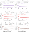 |
Fig. A.1. Similar to Fig. 7 but for the Fermi/LAT detection of intermediate Galactic coordinates 10° ≤|b|≤20° in the upper panels, for the Galactic ridge with 80° ≤|l|≤180° and |b|≤8° in the middle panels, and off plane |b|≥8° in the lower panels. |
Appendix B: DRAGON2 population setup
The total number of sources is the sum of the sources in the disc Nd, the sources located in the central parsec region Nc add those in the bulge Nb:
 (B.1)
(B.1)
Each population follows a distribution:
 (B.2)
(B.2)
where N0 is the normalisation of each population, and ρ(R) and ξ(z) are the (unitless) number densities in the radial direction and perpendicular to the Galactic plane, respectively.
The disc sources follow the profile of the Lorimer distribution (Lorimer et al. 2006):
 (B.3)
(B.3)
where R0 = 8.3 kpc, B = 1.9, C = 5, and ε = 0.18 kpc. The normalisation of the Lorimer distribution is hence given by:
 (B.4)
(B.4)
where we set t = cR/R0, Γ is the Euler (gamma) function and Q is the generalised incomplete gamma function.
The sources of the Galactic centre follow a Gaussian distribution (Mori et al. 2021) whose the normalisation is:
![Mathematical equation: $$ \begin{aligned} N_{0,c} = \frac{N_c}{\sqrt{2\pi } \varepsilon \left[2\sigma _c e^{-\mu _c^2/4\sigma _c^2} + \sqrt{\pi }\mu _c \left(\mathrm{erf} \left(\dfrac{\mu _c}{2\sigma _c}\right)+1\right)\right]}, \end{aligned} $$](/articles/aa/full_html/2024/10/aa50122-24/aa50122-24-eq16.gif) (B.5)
(B.5)
where μc = 2 pc, σc = 20 pc and erf is the error function. This normalisation yields  .
.
Finally, the sources of the bulge follow a spherical distribution (Korol et al. 2018):
 (B.6)
(B.6)
where rb = 0.5 kpc is the characteristic radius of the bulge and  is the spherical distance from the Galactic centre. The normalisation of this distribution is:
 (B.7)
(B.7)
In a Cartesian 3D coordinate system, and for a more realistic distribution, we use the boxy bulge (Cao et al. 2013) that is described by the modified Bessel function of the second kind K0(rs) where
 (B.8)
(B.8)
with x0 = 0.69 kpc, y0 = 0.29 kpc and z0 = 0.27 kpc. The normalisation for the 3D boxy bulge can be written as  . For all the normalisations we assume the Milky Way to extend to some radius of 12 kpc and height 4 kpc.
We define the fraction of sources that are located in the GC with respect to the total number of sources:
 (B.9)
(B.9)
which we allow to vary.
The total source luminosity is
 (B.10)
where fesc is the fraction of CRs escaped from the jets of each individual source, ϕ(fesc) is the PDF of fesc and Pp is the power carried by the protons, which according to A0620−00 is 8.9 × 1034 erg s−1. We calculate N0 from the total number of sources
 (B.11)
and f(E) is the energy distribution of the particles of each source, which we assume to be a power-law E−p with an exponential cutoff at some maximum energy Emax. The power-law index is around 2, and we assume that its probability density follows a Gaussian G(p) with μp = 2.0 and σp = 0.3 (cite particle acceleration papers here). In DRAGON2 we use as an input the quantity N0Q0 (Q0_custom), so we calculate Q0 as
 (B.12)
For the case of a power law f(E) = E−p from Ep, min = 1 GeV to Ep, max = 36 TeV (see Section where we describe the jet model and how we calculate the maximum energy for protons)
Appendix C: CR spectrum
In Fig. C.1, we plot the proton CR spectrum where we show the contribution of the qBHXBs to the detected spectrum. We compare to AMS-02 proton spectrum (Aguilar et al. 2015), the ATIC proton data (Chang et al. 2008), the CREAMIII (Yoon et al. 2017), DAMPE (DAMPE Collaboration 2019), and KASCADE (Apel et al. 2011). The qBHXBs mainly from the disc (because the boxy bulge GeV-TeV protons are subdominant) contribute very insignificantly, with less than 10−10. In Fig. C.2 we show the electron CR spectrum using the AMS-02 electron data (Aguilar et al. 2014), and similar to protons, the contribution is negligible. In the same plot, we show the contribution of both the primary electrons and those produced by the propagation of protons and their interaction with the Galactic gas. We see that the secondary electrons dominate over the primary, but still are not enough to contribute somehow to the detected electron spectrum.
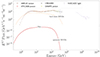 |
Fig. C.1. The contribution of the qBHXBs of a Lorimer-like distribution in the Galactic disc to the proton CR spectrum as detected on Earth. For comparison, we include the contribution of the BHXBs in the hard state from Kantzas et al. (2023b). |
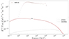 |
Fig. C.2. The contribution of a Lorimer-like distribution of qBHXBs in the Galactic disc to the electron CR spectrum detected on Earth. We plot both the primary electrons (dotted line), namely those that escape the qBHXBs and propagate in the Galaxy, and the secondary electrons that are formed after the inelastic collisions of the propagating proton CRs with the Galactic gas (dotted line). |
All Tables
The free (fitted) parameters of the multi-wavelength spectral modelling fit to A0620−00.
Calculated power carried by the non-thermal protons (p) and electrons (e) and their maximum energy for the two jet models.
All Figures
|
Fig. 1. Best fit with residuals of the multi-wavelength flux density of the 2013 observations of A0620−00 from Dinçer et al. (2017). In the upper panel, we show the result for the case of BHJet, and in the lower panel, we show the case of MLJet. The solid black line shows the total absorbed emission, and the individual components are explained in the legend. |
| In the text | |
|
Fig. 2. Multi-wavelength spectrum of A0620−00 for the case of the BHJet model in the upper panel and for the case of the MLJet model in the lower panel. The solid black line shows the total emitted spectrum, and the individual components are explained in the legends. The radio-to-X-ray data are the same as in Fig. 1. We include the INTEGRAL/SPI, Fermi/LAT, and CTAO point source sensitivities for comparison. |
| In the text | |
|
Fig. 3. Positions of one random realisation of qBHXBs in the sky (left) in Galactic coordinates and the histogram of their distances (right). From top to bottom, we plot the 103 sources at the GC, the 104 boxy bulge, and the 1.2 × 10⁴ Galactic disc. |
| In the text | |
|
Fig. 4. Histogram of the masses of the BH of the qBHXBs. The shaded grey region is adopted from Olejak et al. (2020), from which we derive the Gaussian kernel shown by the solid line. The shaded orange histogram corresponds to 104 boxy bulge qBHXBs (left panel) and 1.2 × 10⁵ disc qBHXBs (right panel) used in this work. |
| In the text | |
|
Fig. 5. Contribution of the prompt emission of the Galactic qBHXBs to the NuSTAR diffuse emission for 1° ≤(l, b)≤3° (Perez et al. 2019). The upper panel shows the assumed model BHJet, and the lower panel shows the MLJet. In both panels, we show the lower and upper limit of the Lorimer-like distribution (1.2 × 10⁴ versus 1.2 × 10⁵ qBHXBs) and the 103 boxy bulge-like sources based on Olejak et al. (2020). The sum of the boxy bulge and the Lorimer-like distribution leads to the total contribution, which we plot with the thin solid line for the upper limit and the thick solid line for the lower limit. The shaded grey region corresponds to the predicted contribution of these qBHXBs to the observed diffuse emission. The insets in both panels show the percentage contribution per energy bin. |
| In the text | |
|
Fig. 6. Similar to Fig. 5, but for the energy band covered by INTEGRAL for (|l|,|b|) ≤ (47.5° ,47.5° ) (Berteaud et al. 2022). We overplot the point source sensitivity of INTEGRAL/SPI on the diffuse emission, as indicated in the legend (Roques et al. 2003), and compare it to individual sources that contribute to the total emission (solid coloured lines for individual sources). We show only sources that lie above the instrument sensitivity. No sources lie above the threshold for MLJet. |
| In the text | |
|
Fig. 7. Similar to Fig. 5, but for the energy band covered by Fermi/LAT, and only for the region around the GC with |l|≤80° and |b|≤8°. |
| In the text | |
|
Fig. 8. Similar to Fig. 5, but for the highest-energy regime of TeV compared to the H.E.S.S. (top left), HAWC (top right), LHAASO (bottom left), and CTAO (bottom right) facilities. For H.E.S.S., HAWC, and LHAASO, we show with solid coloured lines the individual sources that exceed 10−3 of the point source sensitivity, and for CTAO, we show the sources that exceed one-third of the predicted point source sensitivity. For all panels, we only show the case of BHJet because the contribution of sources that follow MLJet is even smaller than pictured here. The inner (outer) region for the case of HAWC is 43° ≤l ≤ 73° and |b|≤2° (|b|≤4°), and the inner (outer) region for the case of LHAASO is 15° ≤l ≤ 125° (125° ≤l ≤ 235°) and |b|≤5°. For CTAO, the sources lie within |l|≤60° and |b|≤3° (Eckner et al. 2023). All the panels have the same axes for comparison. |
| In the text | |
|
Fig. 9. Cumulative distribution of sources per energy flux detected at a characteristic radio frequency of 1.28 GHz. The two histograms correspond to the two assumptions for an upper or lower limit of qBHXBs populating a Lorimer-like distribution in the disc. We show for comparison the detection threshold of radio sources with current facilities, such as MeerKAT and VLA (∼10 μJy). |
| In the text | |
|
Fig. 10. Predicted neutrino flux from the source populations as shown in the legend (also see Fig. 5), assuming that the BHJet jet scenario explains their jet dynamics. The subplot shows the contribution of the total predicted flux to the detected Galactic neutrino diffuse emission by IceCube (IceCube Collaboration 2023). The three different colours represent the three different models used to extract the observed flux. |
| In the text | |
|
Fig. A.1. Similar to Fig. 7 but for the Fermi/LAT detection of intermediate Galactic coordinates 10° ≤|b|≤20° in the upper panels, for the Galactic ridge with 80° ≤|l|≤180° and |b|≤8° in the middle panels, and off plane |b|≥8° in the lower panels. |
| In the text | |
|
Fig. C.1. The contribution of the qBHXBs of a Lorimer-like distribution in the Galactic disc to the proton CR spectrum as detected on Earth. For comparison, we include the contribution of the BHXBs in the hard state from Kantzas et al. (2023b). |
| In the text | |
|
Fig. C.2. The contribution of a Lorimer-like distribution of qBHXBs in the Galactic disc to the electron CR spectrum detected on Earth. We plot both the primary electrons (dotted line), namely those that escape the qBHXBs and propagate in the Galaxy, and the secondary electrons that are formed after the inelastic collisions of the propagating proton CRs with the Galactic gas (dotted line). |
| In the text | |
Current usage metrics show cumulative count of Article Views (full-text article views including HTML views, PDF and ePub downloads, according to the available data) and Abstracts Views on Vision4Press platform.
Data correspond to usage on the plateform after 2015. The current usage metrics is available 48-96 hours after online publication and is updated daily on week days.
Initial download of the metrics may take a while.