© The Authors 2024

1. Introduction

The very-high energy (VHE) gamma-ray source HESS J1745−290, located at the Galactic center, has been observed by several imaging atmospheric Cherenkov telescopes (IACTs), such as CANGAROO, VERITAS, H.E.S.S., and MAGIC (Tsuchiya et al. 2004; Kosack et al. 2004; Aharonian et al. 2004; Albert et al. 2006; HESS Collaboration 2016, 2018; MAGIC Collaboration 2020; Adams et al. 2021). This source is usually characterized by a hard power-law spectrum with a photon index of ∼2.1 and an exponential cutoff at ∼10 TeV. However, its spectral shape is also compatible with a broken power law with the break energy at a few TeV (Aharonian et al. 2009; Adams et al. 2021)¹.

Although several models have been proposed to explain this source, HESS J1745−290 has not yet been associated with a particular astrophysical object. This is mainly because of the limited ∼3′ angular resolution of current IACTs, which translates to ∼10 pc in projected distance from the Galactic center (Funk & Hinton 2008). However, some processes have been proposed: (1) dark matter annihilation in a density cusp at the Galactic center (Hooper et al. 2004; Profumo 2005; Aharonian et al. 2006; Cembranos et al. 2012), (2) inverse Compton emission by relativistic electrons in the pulsar wind nebula G359.95-0.04 (Hinton & Aharonian 2007; Wang et al. 2006), and (3) the decay of neutral pions produced by hadronic collisions of cosmic rays (CRs) accelerated by the central supermassive black hole Sagittarius A* (Sgr A*) with background protons in the interstellar gas (Aharonian & Neronov 2005; Chernyakova et al. 2011; Rodríguez-Ramírez et al. 2019).

In the present work we focus on the last scenario. Although Sgr A* is today a relatively quiescent black hole, it has most likely gone through significantly more active phases in the past. This is suggested by the presence of the Fermi bubbles, which are plausibly caused by intense accretion activity some ∼10⁶ − 10⁷ years ago (Su et al. 2010). Also, the observations of X-ray echoes coming from dense gas in the Galactic center region suggest an intense flaring activity in the past few hundred years (Clavel et al. 2013; Marin et al. 2023). Thus, assuming some efficient accretion-driven CR acceleration mechanism, Sgr A* may be powering HESS J1745−290 as its accelerated CRs propagate away from the Galactic center and interact hadronically with the surrounding gas.

The potentially important role of Sgr A* in producing the TeV emission of HESS J1745−290 is also supported by the diffuse VHE gamma-ray emission from the central molecular zone (CMZ) located in the inner few hundred parsecs of the Galaxy (HESS Collaboration 2016). This emission is correlated with the density of molecular gas, suggesting hadronic emission due to CR collisions with background protons. The CR density profile inferred from this assumption is consistent with a 1/r dependence (where r is the distance to the Galactic center), supporting the radial diffusion of CRs continuously injected from the inner tens of parsecs around the Galactic center². The gamma-ray spectrum of this emission is characterized by a single power law with an index of ∼2.3 up to tens of TeV, without a statistically significant spectral cutoff, as shown by H.E.S.S. and VERITAS (HESS Collaboration 2016; Adams et al. 2021), although some controversy remains due to indications of a spectral turnover around 20 TeV reported by MAGIC (MAGIC Collaboration 2020). The possible lack of a cutoff in the diffuse CMZ emission is interesting, because it allows the possibility of the existence of a PeV proton accelerator, or “PeVatron”, to be present within the inner tens of parsecs of the Galaxy. These observations have thus been considered as strong indications that Sgr A* is operating as a PeVatron (HESS Collaboration 2016), although contributions from other possible CR acceleration systems have also been considered. One possible contribution includes CRs accelerated in the shock fronts of the supernova remnants Sgr A East (HESS Collaboration 2016; Scherer et al. 2022, 2023) and G0.9+01 (Dörner et al. 2024). Another possibility is related to the multiple shocks formed by stellar winds in the Nuclear, Arches, and Quintuplet clusters of young massive stars (Aharonian et al. 2019; Scherer et al. 2022, 2023), with the Arches and Quintuplet clusters being located at a projected distance of ∼25 pc from Sgr A*, while the dynamic center of the Nuclear cluster coincides with it (Hosek et al. 2022).

Even though the scenario in which Sgr A* drives the emissions of both HESS J1745−290 and the CMZ is appealing, one of its main challenges is the clear presence of a spectral turnover (either an exponential cutoff or a spectral break) at a few to ∼10 TeV in HESS J1745−290, which appears to be absent from the CMZ emission. One possible way to alleviate this discrepancy is by invoking the absorption of ≳10 TeV gamma rays from HESS J1745−290 by e⁺e⁻ pair production due to their interaction with the interstellar radiation field (ISRF). Although this absorption is not expected to be important given the known ISRF in the Galactic center (Zhang et al. 2006; Aharonian et al. 2009), its effect may become significant due to clumpiness of the interstellar medium (Guo et al. 2017). Another possibility is simply a relatively recent decrease in the power of CR injection (Liu et al. 2016), which would mean that the diffuse emission is powered by CRs with up to ∼ PeV energies accelerated by Sgr A* ≳10⁴ years ago, and that HESS J1745−290 is associated with a less efficient acceleration period over the last ∼10 − 100 years.

In this paper, we present an alternative scenario, in which the spectral turnover of HESS J1745−290 is caused by an energy-dependent transition in the diffusion regime of CRs injected by Sgr A*. In our model, HESS J1745−290 is caused by CRs experiencing hadronic collisions as they diffuse out through the accretion flow of Sgr A* (r ≲ 0.1 pc). Although the injected CRs in our proposed scenario have an energy distribution given by a single power law up to ∼ PeV energies, the transition in their diffusion regime significantly reduces their number density within the accretion flow for energies of ≳20 TeV. This density reduction in turn imprints a break in the gamma-ray emission spectrum at a few TeV.

Our proposed model requires three basic ingredients:

The first ingredient corresponds to the radial profiles for the density, velocity, and magnetic field strength in the gas at r ≲  1 pc. The gas has been proposed to mainly come from the wind of ∼ 30 Wolf-Rayet (WR) stars, which belong to the Nuclear cluster and orbit around Sgr A* at a distance of ∼0.1 − 1 pc (Cuadra et al. 2006, 2007). These profiles are obtained from previously reported hydrodynamic (Ressler et al. 2018) and magnetohydrodynamic (MHD; Ressler et al. 2020a) simulations of the Sgr A* accretion flow. Interestingly, despite the relatively large magnetic fields used for the stellar winds in the MHD studies, their obtained angle-averaged gas density, temperature, and velocity are largely insensitive to the assumed magnetic field strength and are essentially the same as those found in the hydrodynamic simulations (Ressler et al. 2020a). Because of this, below we refer to both hydrodynamic and MHD results when describing the assumed gas behavior in our model.

A second ingredient is given by the diffusion and advection properties of the CRs within the MHD turbulence in the r ≲ 1 pc region. While the properties of the gas flow are obtained from previous hydrodynamic and MHD simulations, the CR diffusion properties are inferred from previous studies of test-particle CRs propagating in synthetic turbulence, which we assume to be strong (i.e., the mean large-scale magnetic field is much weaker than the fluctuating field), isotropic, and with a Kolmogorov spectrum (Subedi et al. 2017; Mertsch 2020; Dundovic et al. 2020). One of the main assumptions made in this work is that the mean field is much weaker than the turbulent field, which allows us to neglect a possible anisotropy in the CR diffusion, as has been found in test-particle simulations (see, e.g., Reichherzer et al. 2022a,b, 2023).

Finally, we assume a flux of centrally injected CRs whose spectral distribution corresponds to a single power law whose index, normalization, and maximum energy (reaching ∼PeV energies) are consistent with estimates obtained from the diffusive CMZ emission (HESS Collaboration 2016).

Most parameters in our model are thus relatively well constrained by previously reported hydrodynamic and MHD simulations of the Sgr A* accretion flow, as well as by the spectral properties of the CMZ emission. The only exception is the coherence length l_c of the MHD turbulence in the accretion flow, which, despite playing a critical role in the diffusion properties of the CRs, is a poorly known parameter of our model. Interestingly, we find that by choosing l_c ∼ (1 − 3)  ×  10¹⁴ cm, our model is capable of matching the main spectral features of HESS J1745−290 fairly well, including its spectral turnover, while being consistent with the injected CR spectrum required to reproduce the CMZ emission.

We note that, in our model, the CR injection occurs within a radius of r ≲ 10R_g, where R_g is the gravitational radius of the black hole (or Schwarzschild radius, which in the case of Sgr A* is R_g ≈ 10¹² cm). This is justified by the fact that electron acceleration events in Sgr A* are routinely inferred in association with near-infrared and X-ray flares (likely powered by reconnection events; Ponti et al. 2017; Subroweit et al. 2020; Scepi et al. 2022), whose emission regions have been located at a few R_g from the central black hole (GRAVITY Collaboration 2018). Although this injection region may itself be the source of significant gamma-ray emission (Rodríguez-Ramírez et al. 2019), our work specifically focuses on the emission produced at r ≳ 10R_g (which, as we show, is dominated by r ≫ 10R_g).

Our paper is organized as follows. In Sect. 2, we calculate the CR density as a function of radius and energy within the accretion flow of Sgr A*, considering the diffusion properties of CRs in that region, as well as the velocity profile of the background gas. In Sect. 3, we calculate the gamma-ray emission resulting from the hadronic interaction of the CRs with the background gas. In Sect. 4, we verify the consistency of the assumptions made in our calculations. In Sect. 5, we provide a discussion regarding CR diffusion timescales and how they could be used to observationally test our model. Finally, our conclusions are presented in Sect. 6.

2. Cosmic ray density model

In this work, we assume that CRs are ultrarelativistic protons being steadily injected near the event horizon of Sgr A* and propagate to larger radii r through its accretion flow. This accretion flow originates mainly from the gas being injected by a cluster of WR stars orbiting at ∼0.1 − 1 pc from Sgr A* (Cuadra et al. 2006, 2007). The CR transport equation can be written as (e.g., Strong et al. 2007)

$$\begin{array}{cc}\hfill \frac{\partial }{\partial t}(\frac{d{n}_{\mathit{CR}}}{\mathit{dE}}(E,\mathit{r},t))& =S(E,\mathit{r},t)+\mathrm{\nabla }·\{D(E,\mathit{r})\mathrm{\nabla }(\frac{d{n}_{\mathit{CR}}(E,\mathit{r},t)}{\mathit{dE}})\hfill \end{array}$$(1)

$$\begin{array}{cc}\hfill & -\mathit{v}(\mathit{r},t)\frac{d{n}_{\mathit{CR}}(E,\mathit{r},t)}{\mathit{dE}}\},\hfill \end{array}$$(2)

where dn_CR/dE(E, r, t) is the CR density per unit energy E as a function of position r and time t. The term S(E, r, t) is the source term that quantifies CR injection, D(E, r) is the CR diffusion coefficient and v(r, t) is the gas velocity, which allows advection to contribute to CR propagation. In Eq. 1 we neglect possible CR energy gains (e.g., due to stochastic acceleration) and energy losses (we verified that energy losses are indeed small by comparing the CR diffusion times found in Sect. 5 with the cooling times due to hadronic CR interactions). For simplicity, and as a first approach to this problem, in this work we solve Eq. 1 assuming a stationary and spherically symmetric CR density model. In what follows, we describe the parameters and assumptions regarding CR injection and transport.

2.1. Cosmic-ray injection

In our model, we assume that the CR injection occurs only within a radius of r < 10R_g, and solve for dn_CR/dE(E, r) at r > 10R_g. Thus, our calculations do not require the exact form of the source term S(E, r) in Eq. 1, but only the total number of injected CRs per unit energy E and per unit time t within the injection region, which is given by

$$\begin{array}{c}\hfill \mathrm{d}N/\mathrm{d}\mathrm{d}t(E)=4\pi {\displaystyle {\int }_0^{10R_g}}r{r}^{2}S(E,r).\end{array}$$(3)

For this, we assume a power-law dependence of

$$\begin{array}{c}\hfill \frac{\mathrm{d}N}{\mathrm{d}E\mathrm{d}t}(E)=2.3\times {10}^{36}f(q,E_{\max })\widehat{Q}{\left(\frac{E}{1\mathrm{TeV}}\right)}^{-q}{\mathrm{erg}}^{-1}{\mathrm{s}}^{-1},\end{array}$$(4)

for E smaller than a maximum energy E_max, and dN/(dEdt) = 0 otherwise. Here, q is the spectral index of the injected CR spectrum, $\widehat{Q}$ is a parameter that quantifies the injection power, and

$$\begin{array}{c}\hfill f(q,E_{\max })=\frac{2-q}{{\left(\frac{E_{\max }}{1\mathrm{TeV}}\right)}^{2-q}-{10}^{2-q}}\mathrm{if}q\ne 2,\end{array}$$(5)

while, if q = 2,

$$\begin{array}{c}\hfill f(q=2,E_{\max })={[ln\left(\frac{E_{\max }}{1\mathrm{TeV}}\right)-ln(10)]}^{-1},\end{array}$$(6)

and so the CR injection power for E ≥ 10 TeV is

$$\begin{array}{c}\hfill Q(E>10\mathrm{TeV})=6\times {10}^{36}\widehat{Q}{\mathrm{erg}\mathrm{s}}^{-1}.\end{array}$$(7)

2.2. Cosmic-ray transport

As our model is stationary and assumes spherical symmetry, integrating Eq. 1 over a spherical volume of radius r, and considering the definition of dN/dEdt(E) provided by Eq. 3, we obtain

$$\begin{array}{c}\hfill \frac{\mathrm{d}N}{\mathrm{d}E\mathrm{d}t}(E)=4\pi r^2(v_{\mathrm{gas}}(r)\frac{\mathrm{d}{n}_{\mathrm{CR}}}{\mathrm{d}E}(E,r)-D(E,r)\frac{\partial }{\partial r}\left(\frac{\mathrm{d}{n}_{\mathrm{CR}}}{\mathrm{d}E}(E,r)\right)),\end{array}$$(8)

where v_gas(r) is the angle-averaged gas velocity in the radial direction at a radius r. We see that both diffusion and advection are expected to contribute to CR propagation. However, below we show that, in our model, diffusion is the dominant process at r ≲ 0.07 pc for all energies of interest, while for r ≳ 0.07 pc advection dominates for CRs with sufficiently low energies. Thus, as an approximation, in our calculations of dn_CR/dE(E, r) from Eq. (8) we impose that, at a given radius r and energy E, CRs are transported entirely by one process, either diffusion or advection (i.e., keeping only one of the two terms on the right-hand side of Eq. (8)), depending on which one is more efficient. This is done by comparing the radial gas velocity v_gas to the diffusion velocity,

$$\begin{array}{c}\hfill v_{\mathrm{diff}}(E,r)\equiv \frac{D(r,E)}{r},\end{array}$$(9)

and neglecting the diffusion (advection) term on the right-hand side of Eq. (8) if v_gas (v_diff) is larger³. We note that CRs can also be advected by the turbulent motions of the gas, giving rise to turbulent diffusion. We show below that this effect can be neglected for the cases of interest (see Sect. 4), and so CR transport in our model is determined by the properties of D(E, r) and v_gas(r).

2.2.1. Diffusion model

In order to model D(E, r), we use results from previous test particle simulations of CRs propagating in synthetic MHD turbulence (i.e., magnetostatic turbulence with a prespecified spectrum), which we assume to be strong in the sense that the rms magnetic field magnitude is much larger than any large-scale mean field, is isotropic, and has a Kolmogorov spectrum (Subedi et al. 2017; Mertsch 2020; Dundovic et al. 2020). This turbulence is characterized by a coherence length l_c, which is the spatial scale within which most of the turbulent magnetic energy is contained (Fleishman & Toptygin 2013). These simulations identify two main diffusion regimes, which are also consistent with theoretical diffusion models (Aloisio & Berezinsky 2004; Subedi et al. 2017). The “high-energy diffusion”(HED) regime occurs when the energy of the CRs is such that their Larmor radii R_L satisfy R_L ≫ l_c (R_L = E/eB, where e is the proton electric charge and B is the magnitude of the magnetic field), while the “low-energy diffusion”(LED) regime occurs when R_L ≪ l_c. We obtain expressions for the effective mean free path λ_mfp of CRs in these two diffusion regimes from Subedi et al. (2017) (where a broken power-law shape is assumed for the turbulence spectrum). Figure 1 of Subedi et al. (2017) shows that, for R_L ≪ l_c (LED), λ_mfp is given by

$$\begin{array}{c}\hfill {\lambda }_{\mathrm{mfp}}\approx 0.4l_c^{2/3}{R}_L^{1/3},\end{array}$$(10)

while for R_L ≫ l_c (HED),

$$\begin{array}{c}\hfill {\lambda }_{\mathrm{mfp}}\approx 2l_c^{-1}{R}_L^2,\end{array}$$(11)

with a smooth transition for R_L ∼ l_c. (In Appendix B we give heuristic derivations for the dependence on l_c and R_L in these two limiting regimes.) We note that, as Eqs. 10 and 11 are approximate expressions obtained from Fig. 1 of Subedi et al. (2017), their normalizations should only be considered to have an accuracy at the ∼10% level. Another approximation is that, in our calculations, the transition in the λ_mfp behavior at R_L ∼ l_c is satisfied by assuming

$$\begin{array}{c}\hfill {\lambda }_{\mathrm{mfp}}=\{\begin{array}{cc}0.4l_c^{2/3}{R}_L^{1/3}\hfill & \mathrm{for}{R}_L\le 0.38l_c,\hfill \\ 2l_c^{-1}{R}_L^2\hfill & \mathrm{for}{R}_L>0.38l_c.\hfill \end{array}\end{array}$$(12)

Thus, in order to obtain D(E, r) = λ_mfp(E, r)c/3 (where c is the speed of light), we need an expression for the rms magnitude of the magnetic field B as a function of r. Based on the MHD simulations of the Sgr A* accretion flow of Ressler et al. (2020a), we assume it to have a power-law profile,

$$\begin{array}{c}\hfill B(r)=10\widehat{B}{\left(\frac{r}{10R_g}\right)}^{-n}\mathrm{G},\end{array}$$(13)

where n ≈ 1, while $\widehat{B}$ is a factor of order unity, and is relatively independent of the conditions assumed for the wind of the WR stars. From this, we obtain a space- and energy-dependent Larmor radius of

$$\begin{array}{c}\hfill R_L\approx 3.3\times {10}^8{\widehat{B}}^{-1}\frac{E}{\mathrm{TeV}}{\left(\frac{r}{10R_g}\right)}^n\mathrm{cm}.\end{array}$$(14)

In contrast, the value of the coherence length l_c in the accretion flow is highly uncertain. In order to model the possible radial dependence of this parameter, we also assume a power-law shape for it, with

$$\begin{array}{c}\hfill l_c(r)={10}^{14}{\widehat{l}}_c{\left(\frac{r}{0.07\mathrm{pc}}\right)}^m\mathrm{cm},\end{array}$$(15)

where ${\widehat{l}}_c$ and m are free parameters of our model.

Thus, the diffusion coefficient in the LED regime, R_L ≪ l_c, is

$$\begin{array}{c}\hfill \begin{array}{cc}\hfill D_{\mathrm{LED}}(E,r)=& 6\times {10}^{21}{(2.1\times {10}^4)}^{-2m/3}{\widehat{l}}_c^{2/3}{\widehat{B}}^{-1/3}\hfill \\ \hfill & \times {\left(\frac{E}{1\mathrm{TeV}}\right)}^{1/3}{\left(\frac{r}{10R_g}\right)}^{\frac{1}{3}(n+2m)}{\mathrm{cm}}^2{\mathrm{s}}^{-1},\hfill \\ \hfill \end{array}\end{array}$$(16)

while in the HED regime, R_L ≫ l_c,

$$\begin{array}{c}\hfill \begin{array}{cc}\hfill D_{\mathrm{HED}}(E,r)=& 2\times {10}^{13}{(2.1\times {10}^4)}^m{\widehat{l}}_c^{-1}{\widehat{B}}^{-2}\hfill \\ \hfill & \times {\left(\frac{E}{1\mathrm{TeV}}\right)}^2{\left(\frac{r}{10R_g}\right)}^{2n-m}{\mathrm{cm}}^2{\mathrm{s}}^{-1}.\hfill \\ \hfill \end{array}\end{array}$$(17)

2.2.2. Advection model

In order to model v_gas(r), we need to characterize the gas dynamics within the Sgr A* accretion flow. For this, we use the hydrodynamic simulations presented by Ressler et al. (2018), which assume that the gas is mainly provided by the wind of a cluster of WR stars orbiting at 0.1 − 1 pc from Sgr A*. Interestingly, these simulations show no significant differences with the MHD simulations of (Ressler et al. 2020a) when angle-averaged quantities are considered. For simplicity, we assume that this gas is a plasma composed of electrons and protons of equal number density n_e(r) = n_p(r) = n_gas(r). The profile of the gas density n_gas is obtained from Fig. 11 of Ressler et al. (2018), which provides quantities averaged over angle and time (over the 100 years previous to the present day). This density profile can be approximated by⁴

$$\begin{array}{c}\hfill n_{\mathrm{gas}}(r)=\{\begin{array}{cc}25{\left(\frac{r}{0.4\mathrm{pc}}\right)}^{-1}{\mathrm{cm}}^{-3}& \mathrm{if}r\le 0.4\mathrm{pc},\\ 25{\left(\frac{r}{0.4\mathrm{pc}}\right)}^{-2}{\mathrm{cm}}^{-3}& \mathrm{if}r>0.4\mathrm{pc}.\end{array}\end{array}$$(18)

We note that, according to Fig. 11 of Ressler et al. 2018, the n_gas(r) profile at 0.07 pc ≲ r ≲ 0.4 pc is steeper than n_gas(r)∝r⁻¹. However, we show in Sect. 3.1 that the gamma-ray emission from this region is expected to be ≲20 − 30% of the total emission at all energies. Therefore, as a reasonable approximation, we use Eq. 18 to describe n_gas(r) at all radii smaller than 0.4 pc.

Regarding the gas velocity, Ressler et al. (2018) identify four regions within the accretion flow:

Region I: This is the outflow-dominated region defined by r > 0.4 pc. Here, the gas moves away from the Galactic center and v_gas(r) is essentially given by the speed of the WR star winds.

Region II: Located at 0.07 pc < r < 0.4 pc, this region corresponds to the “feeding” region, where most of the gas injection from the WR star winds occurs, and in which the gas motion predominantly points away from the Galactic center.

Region III: Corresponds to a “stagnation” region at 0.01pc < r < 0.07 pc, which is characterized by inflows and outflows of gas, with the net mass-accretion rate nearly vanishing.

Region IV: Corresponds to an inflow-dominated region at r < 0.01 pc, where the mass-accretion rate Ṁ is roughly constant.

In region IV, we consider a constant mass-accretion rate Ṁ ≈ 10⁻⁸ M_⊙/yr (Ressler et al. 2020b; Dexter et al. 2020), with which we find that

$$\begin{array}{cc}\hfill v_{\mathrm{gas}}(r)& =-\frac{\dot{M}}{4\pi r^2{n}_{\mathrm{gas}}(r)m_p}\hfill \\ \hfill & \approx -3\times {10}^4{\left(\frac{r}{0.01\mathrm{pc}}\right)}^{-1}\mathrm{cm}/\mathrm{s},\hfill \end{array}$$(19)

where m_p is the proton mass.

In region III, the average radial velocity of the gas tends to cancel out, and therefore CR transport should not be significantly affected by advection. In what follows, we neglect the effect of v_gas(r) for regions III and IV, for which we assume that CR transport is dominated by diffusion. The validity of this assumption is verified in Sect. 4.

In regions I and II (r > 0.07 pc), we can estimate v_gas from Fig. 18 in Ressler et al. (2018), which can be approximated by

$$\begin{array}{c}\hfill v_{\mathrm{gas}}(r)\approx \{\begin{array}{c}700(r/0.4\mathrm{pc})\mathrm{km}/\mathrm{s}\mathrm{for}0.07\mathrm{pc}<r<0.4\mathrm{pc}\hfill \\ 700\mathrm{km}/\mathrm{s}\mathrm{for}r>0.4\mathrm{pc}.\hfill \end{array}\end{array}$$(20)

In this case, v_gas dominates CR transport for sufficiently low energies, while diffusion dominates for higher-energy particles. Thus, for 0.07 pc < r < 0.4 pc, we consider diffusive transport at energies for which v_diff > v_gas, and advective transport in the opposite case. For simplicity, at r > 0.4 pc, we assume the same transport mechanism that dominates at r = 0.4 pc, which, depending on E, could either be HED or advection. As discussed in Sect. 4.2, this should not affect our main results.

2.3. Previous constraints on parameters

As our purpose is to build a model for the point source HESS J1745−290 that is compatible with the diffuse emission from the CMZ, the injection parameters q, $\widehat{Q}$, and E_max have to obey restrictions related to the CMZ emission. This emission has been found to be consistent with a CR proton spectral index of Γ_p ≈ 2.3 (HESS Collaboration 2016). This, however, does not correspond to the index q of the injected CRs, as the CR spectrum in the CMZ is also affected by the energy-dependent residence time of the CRs in this region, which is inversely proportional to the CR diffusion coefficient in the CMZ, which itself is assumed to have a power-law shape of D_CMZ(E)∝E^δ. This implies that Γ_p = q + δ, with the value of δ likely between δ ≈ 1/3 and 1/2, as expected for Kolmogorov and Kraichnan types of magnetic turbulence, respectively (Aharonian 2004). Thus, a reasonable expectation for q is ≈2. Also, making different assumptions regarding the magnitude of D_CMZ(E), HESS Collaboration (2016) and Scherer et al. (2022) found the CR injection power for E > 10 TeV to be Q(E > 10 TeV)≈8 × 10³⁷erg s⁻¹ and 3 × 10³⁶erg s⁻¹, implying $\widehat{Q}\approx 13$ and 0.5, respectively. Additionally, the spectrum of the diffuse emission restricts the maximum CR energy to E_max ≳ 1 PeV (HESS Collaboration 2016; Adams et al. 2021).

Further parameter restrictions can be obtained from previous MHD simulations of the Sgr A* accretion flow. For instance, Ressler et al. (2018) show that assuming a beta parameter in the winds of the WR stars β_W = 10⁴, the magnetic field near Sgr A* reaches the value B(r = 10R_g)≈10 G ($\widehat{B}\approx 1$), and the parameter n (defined in Eq. (13)) is approximately n ≈ 1. In the case of β_W = 10², these latter authors obtain almost the same $\widehat{B}\approx 1$, while B(r = 0.1 pc) is approximately a factor 4 larger than in the β_W = 10⁴ case. For our assumed power-law dependence B ∝ r⁻ⁿ (Eq. (13)), the latter implies n ≈ 0.9.

Given these considerations, below we restrict our analysis to cases with $\widehat{B}=1$ and q = 2, and consider two possible values for n, namely n = 1 and 0.9. We show below that, with these choices, our model can reproduce the main features of the emission from HESS J1745−290 relatively well if $\widehat{Q}\approx 6-13$ and E_max ≳ 1 PeV, which respects the restrictions related to the diffuse CMZ emission provided by HESS Collaboration (2016). Regarding the more uncertain parameters ${\widehat{l}}_c$ and m, we show that fitting the data of HESS J1745−290 is strongly dependent on ${\widehat{l}}_c$ being in the range of ${\widehat{l}}_c\approx 1-3$ (for n = 1 and 0.9, respectively), while m must be small (m ≲ 0.3). In other words, the coherence length l_c must depend only weakly on r.

2.4. Cosmic-ray density profiles

Considering our assumptions regarding CR injection and transport described in Sect. 2.1 and Sect. 2.2, we solve Eq. (8) assuming continuity in dn_CR/dE at the transition between regions dominated by diffusion and by advection⁵. Figure 1 shows examples of the CR density profile for two combinations of parameters (Cases 2 and 4b in Table 1), where we can identify the three main transport regimes mentioned above:

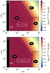Fig. 1. Cosmic-ray density per unit energy dnCR/dE as a function of the radial coordinate r (horizontal axis) and the CR energy E (vertical axis) for cases 2 (panel a) and 4b (panel b) specified in Table 1. The color scale gives log10(E7/3rξdnCR/dE) in cgs units (with ξ = 4/3 in panel a and ξ = 1.3 in panel b), and the dashed lines mark the boundaries between the three CR transport regimes discussed in the text, namely the low-energy diffusion (LED), high-energy diffusion (HED), and advection-dominated (AD) regimes.

(i) Low-energy diffusive (LED) regime: In this region, CR transport is dominated by diffusion, with λ_mfp in the R_L < 0.38 l_c regime of Eq. (12). Solving Eq. (8) in that regime, we obtain:

$$\begin{array}{c}\hfill \begin{array}{cc}\hfill \frac{\mathrm{d}{n}_{\mathrm{CR}}}{\mathrm{d}E}(E,r)=& 3{(2.1\times {10}^4)}^{2m/3}\widehat{Q}{\widehat{l}}_c^{-2/3}{\widehat{B}}^{\frac{1}{3}}\frac{f(q,E_{\max })}{1+\frac{1}{3}(n+2m)}\hfill \\ \hfill & \times {\left(\frac{E}{1\mathrm{TeV}}\right)}^{-q-\frac{1}{3}}{\left(\frac{r}{10R_g}\right)}^{-(1+\frac{1}{3}(n+2m))}{\mathrm{erg}}^{-1}{\mathrm{cm}}^{-3}.\hfill \end{array}\end{array}$$(21)

For simplicity, Eq. (21) does not include the terms that ensure continuity of dn_CR/dE at the boundaries between regions dominated by different transport regimes, which are subdominant. These continuity terms are, however, included in the calculation shown in Fig. 1 as well as in the gamma-ray emission calculations shown in Sect. 3. In Appendix C, we provide the full expression for dn_CR/dE in the LED regime, including the boundary terms.

(ii) High-energy diffusive (HED) regime: In this case, CR transport is also dominated by diffusion, but with λ_mfp in the R_L > 0.38 l_c regime of Eq. (12). In this case, the CR density is given by

$$\begin{array}{c}\hfill \begin{array}{cc}\hfill \frac{\mathrm{d}{n}_{\mathrm{CR}}}{\mathrm{d}E}(E,r)=& {10}^9{(2.1\times {10}^4)}^{-m}\widehat{Q}{\widehat{l}}_c{\widehat{B}}^2\frac{f(q,E_{\max })}{1+2n-m}\hfill \\ \hfill & \times {\left(\frac{E}{1\mathrm{TeV}}\right)}^{-q-2}{\left(\frac{r}{10R_g}\right)}^{-(1+2n-m)}{\mathrm{erg}}^{-1}{\mathrm{cm}}^{-3},\hfill \\ \hfill \end{array}\end{array}$$(22)

dropping off much faster with increasing r (or increasing E), as seen in the upper right corner of Fig. 1. (Here, we are also excluding subdominant terms that ensure continuity of dn_CR/dE, but we provide the full expression in Appendix C.)

(iii) Advection-dominated (AD) regime: In this regime, CR propagation is dominated by advection, and their density is given by

$$\begin{array}{c}\hfill \begin{array}{cc}\hfill \frac{\mathrm{d}{n}_{\mathrm{CR}}}{\mathrm{d}E}(E,r)=& 3\times {10}^6\widehat{Q}f(q,E_{\max }){\left(\frac{E}{1\mathrm{TeV}}\right)}^{-q}\hfill \\ \hfill & \times {\left(\frac{r}{10R_g}\right)}^{-3}{\mathrm{erg}}^{-1}{\mathrm{cm}}^{-3}\hfill \end{array}\end{array}$$(23)

for 0.07 pc ≤r≤ 0.4 pc, and

$$\begin{array}{c}\hfill \begin{array}{cc}\hfill \frac{\mathrm{d}{n}_{\mathrm{CR}}}{\mathrm{d}E}(E,r)=& 21\widehat{Q}f(q,E_{\max }){\left(\frac{E}{1\mathrm{TeV}}\right)}^{-q}\hfill \\ \hfill & \times {\left(\frac{r}{10R_g}\right)}^{-2}{\mathrm{erg}}^{-1}{\mathrm{cm}}^{-3}\hfill \end{array}\end{array}$$(24)

for r > 0.4 pc, where again in both cases the CR density drops off much faster with increasing r than in the LED regime, as seen in the lower right corner of Fig. 1. (No boundary terms are neglected in Eqs. (23) and (24).)

As seen in Figure 1, high-energy CRs diffusing out from the central source undergo a transition from the LED regime to the HED regime at an energy-dependent critical radius r_C determined by the condition R_L = 0.38 l_c, yielding

$$\begin{array}{c}\hfill r_C(E)=0.07{\left[\frac{1.3\times {10}^5{\widehat{l}}_c\widehat{B}}{{(2.1\times {10}^4)}^n}\right]}^{\frac{1}{n-m}}{\left(\frac{E}{\mathrm{TeV}}\right)}^{-\frac{1}{n-m}}\mathrm{pc},\end{array}$$(25)

which is marked by the diagonal dashed lines in the high-energy part of Figs. 1a and 1b. At lower energies, instead, CRs transit from the LED regime to the advective regime at a fixed radius r = 0.07 pc. The energy separating these two types of transition, E_C, is determined by r_C(E_C) = 0.07 pc (corresponding to the inner boundary of the feeding region), which yields

$$\begin{array}{c}\hfill E_C=6.2{(2.1\times {10}^4)}^{1-n}{\widehat{l}}_c\widehat{B}\mathrm{TeV}.\end{array}$$(26)

Figures 1a and 1b also show that, at energies of E > E_C, advection continues to be dominant over HED for r > 0.07 pc until an energy E^* ∼ (2 − 3)E_c, after which HED dominates at r > 0.07 pc. We note that the maximum energy at which advection dominates for r > 0.07 pc is constant in Case 2 (Fig. 1a), but has a weak dependence on r in Case 4b (Fig. 1b). This is because, in the range 0.07pc < r < 0.4pc, making v_gas(r) equal to v_diff(E, r) in the HED regime, we obtain

$$\begin{array}{c}\hfill \frac{E}{\mathrm{TeV}}=15.8{(2.1\times {10}^4)}^{-m/2}{\widehat{l}}_c^{1/2}\widehat{B}(\frac{r}{10R_g}{)}^{1-n+m/2}.\end{array}$$(27)

This implies that in Case 2 (n = 1, m = 0), the limit between the AD and HED regimes is simply given by E = E^*, while in Case 4b (n = 0.9, m = 0), this energy becomes E ∝ r^0.1. For r > 0.4 pc, we assume, for simplicity, that CR transport is dominated by the same process that dominates at r = 0.4 pc (which explains why in Figure 1b the energy that divides the HED and AD regimes becomes constant at r > 0.4 pc). We show in Sect. 4.2 that this approximation does not affect our results, given that emission at r > 0.4 pc is negligible in our model.

3. Gamma-ray emission

Using the CR density determined in Sect. 2, in this section we calculate the gamma-ray spectrum due to the decay of neutral pions (π⁰) produced in collisions between the CRs and the background gas, both assumed to be composed of protons. Following Aharonian (2004), the gamma-ray flux per unit gamma-ray energy E_γ received at Earth is given by

$$\begin{array}{c}\hfill \begin{array}{cc}\hfill {\mathrm{\Phi }}_{\gamma }(E_{\gamma })=& \frac{2c}{d^2{\kappa }_{\pi }}{\int }_{E_{\pi ,\min }}^{\infty }\mathrm{d}{E}_{\pi }\frac{{\sigma }_{\mathit{pp}}(E)}{\sqrt{E_{\pi }^2-{(m_{\pi }{c}^2)}^2}}\hfill \\ \hfill & \times {\int }_{r_{\min }}^{\infty }\mathrm{d}r{r}^2{n}_{\mathrm{gas}}(r)\frac{\mathrm{d}{n}_{\mathrm{CR}}}{\mathrm{d}E}(E,r),\hfill \end{array}\end{array}$$(28)

where $E_{\pi ,\text{min}}=E_{\gamma }+m_{\pi }^2{c}^4/4E_{\gamma }$, $E=m_p{c}^2+\frac{E_{\pi }}{{\kappa }_{\pi }}$, E_π is the energy of the neutral pion produced in the collisions, m_p and m_π are the proton and pion masses, κ_π ≈ 0.17 is the mean fraction of the CR kinetic energy transferred to neutral pions in the collisions (Aharonian 2004), d ≈ 8 kpc is the distance between Sgr A* and the Earth, and r_min is the minimum radius considered for the emissivity calculation. Unless stated otherwise, we take r_min = 10¹³ cm ≈10 R_g in all our calculations. The cross-section for π⁰ production through proton-proton collisions in a proton reference frame is given by (Aharonian 2004)

$$\begin{array}{c}\hfill {\sigma }_{\mathit{pp}}(E)\approx 4\times {10}^{-26}(1+0.04ln\frac{E-m_p{c}^2}{\mathrm{TeV}}){\mathrm{cm}}^2.\end{array}$$(29)

As we are interested in very-high-energy protons, with E ≳ 1 TeV, we neglect the proton and pion masses in all calculations.

3.1. Behavior of the gamma-ray spectrum

Figure 2 shows the differential gamma-ray flux as a function of r and E_γ for Case 2 of Table 1. This flux is clearly in correspondence with the CR density shown in Fig. 1, considering the approximate energy rescaling E_γ ≈ κ_πE. The fact that dn_CR/dE drops off more quickly as a function of r in the HED and AD regimes than in the LED regime show that the gamma-ray flux is dominated by the CRs in the LED regime for any value of E_γ, with a maximum around the transition from the LED to the HED or AD regimes. This means that, in our model, the emission is dominated by r ∼ 0.07 pc for E_γ ≲ 3 TeV, and by 3 × 10⁻⁴ pc ≲r ≲ 0.07 pc (equivalent to 10³R_g ≲ r ≲ 2 × 10⁵R_g) for 3 TeV ≲E_γ ≲ 200 TeV. In other words, the gamma-ray emission should only be significant in the range 10³R_g < r < 0.07 pc. This can be seen from Fig. 3, which shows the total emission spectrum for Case 2 (blue line) and compares it with the contributions from r > 0.4 pc (solid purple line) and from 0.07 pc < r < 0.4 pc (dashed purple line). We see that the emissions from these two ranges of radii only account for at most ∼20 − 30% of the total emission at all the energies considered. Furthermore, one can also see from Fig. 4 that the resulting spectrum (up to ∼100 TeV) for Case 2 is quite insensitive to the choice of r_min as long as this parameter is in the range ∼(10 − 10³) R_g, confirming that most of the emission comes from r ≳ 10³R_g.

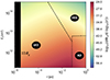Fig. 2. Differential gamma-ray flux per logarithmic interval of r, dΦγ/dlog10(r), as a function of Eγ and r for Case 2 in Table 1.

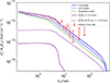Fig. 3. Full and approximate models for the gamma-ray spectrum of HESS J1745−290 with the parameters of Case 2 of Table 1. The solid blue line represents the total gamma-ray emission calculated from the full model. The dashed blue line is the “LED model”, considering only the emission from CRs in the LED regime. The dashed green line shows our simplified model, given by Eqs. (30) and (31). The solid and dashed purple lines represent the contributions from CRs at r > 0.4 pc and 0.07 pc < r < 0.4 pc, respectively. The red dots correspond to the H.E.S.S. measurements (HESS Collaboration 2016).

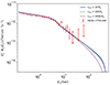Fig. 4. Gamma-ray spectra for Case 2 of Table 1 for different minimum radii rmin from which the gamma-ray emission is integrated (see Eq. (28)). The red dots correspond to the H.E.S.S. measurements of the source HESS J1745−290 (HESS Collaboration 2016).

From Fig. 2 we also see that, for CR energies E > E_C, the LED region is constrained to progressively smaller radii r_C(E) as E increases, thus progressively decreasing the effective emitting volume. This causes a break in the gamma-ray spectrum (obtained by integrating the flux over the whole volume out to r → ∞ and shown as the solid blue line in Fig. 3) at E_γ, b ∼ κ_πE_C, beyond which it decreases more steeply, as in the observed spectrum of HESS J1745−290.

The hypothesis that the gamma-ray spectrum is essentially determined by the shape of the LED region in Fig. 1 is confirmed by recalculating Φ(E_γ) considering only the gamma-ray emission from CRs in this regime (i.e., setting dn_CR/dE = 0 in the HED and AD regimes). This calculation is shown by the dashed blue line in Fig. 3, which shows a similar broken power-law behavior as in the full calculation represented by the solid blue line. Thus, the predicted emission in our model is indeed determined by the CRs in the LED regime, and its broken power-law behavior is a consequence of the energy-dependent transition in the CR diffusion regime at r_C(E) for E > E_C.

3.2. Simplified model

In order to understand how the main features of the HESS J1745−290 spectrum restrict our model parameters, it is useful to provide approximate analytical expressions for our calculated gamma-ray emission. As this emission is dominated by CRs in the LED regime, it can be approximated by considering only the contribution from that regime. For further simplicity, we approximate the CR density in the LED regime by Eq. (21) (neglecting subdominant terms that ensure continuity with the other regimes), ignore the (weak) energy-dependence of σ_pp by fixing E = 1 TeV in Eq. (29), and integrate Eq. (28) from E_π = E_π, min = E_γ to E_π, max = +∞ and from r = 0 to r = 0.07 pc for E_γ < E_γ, b and to r = r_C(E) for E_γ > E_γ, b. (We note that the integral is dominated by the largest radii and the smallest energies over which it integrates.) This way, we obtain relatively simple expressions for Φ_γ(E_γ), which preserve the main features of our model, while showing the effect of the model parameters on the emitted spectrum. For E_γ ≲ E_γ, b,

$$\begin{array}{c}\hfill \begin{array}{cc}\hfill {\mathrm{\Phi }}_{\gamma }(E_{\gamma })\approx & 1.3\times {10}^{-9}{(2.1\times {10}^4)}^{-\frac{n}{3}}\frac{f(q,E_{\max })\widehat{Q}{\widehat{l}}_c^{-\frac{2}{3}}{\widehat{B}}^{\frac{1}{3}}}{1-\frac{1}{9}{(n+2m)}^2}\hfill \\ \hfill & \times \frac{{\kappa }_{\pi }^{q-\frac{2}{3}}}{q+\frac{1}{3}}{\left(\frac{E_{\gamma }}{\mathrm{TeV}}\right)}^{-q-\frac{1}{3}}{\mathrm{TeV}}^{-1}{\mathrm{cm}}^{-2}{\mathrm{s}}^{-1},\hfill \end{array}\end{array}$$(30)

while, for E_γ ≳ E_γ, b,

$$\begin{array}{c}\hfill \begin{array}{cc}\hfill {\mathrm{\Phi }}_{\gamma }(E_{\gamma })\approx & 1.5\times {10}^{-10}6.2^{-\frac{m}{n-m}}{(2.1\times {10}^4)}^{-\frac{m(2-n)}{n-m}}\frac{f(q,E_{\max })\widehat{Q}}{1-\frac{1}{9}{(n+2m)}^2}\hfill \\ \hfill & \times \frac{{\kappa }_{\pi }^{q+\frac{1-n}{n-m}}}{q+\frac{1-m}{n-m}}{\widehat{l}}_c^{\frac{1-n}{n-m}}{\widehat{B}}^{\frac{1-m}{n-m}}{\left(\frac{E_{\gamma }}{\mathrm{TeV}}\right)}^{-q-\frac{1-m}{n-m}}{\mathrm{TeV}}^{-1}{\mathrm{cm}}^{-2}{\mathrm{s}}^{-1},\hfill \end{array}\end{array}$$(31)

both of which are represented by the dashed green line in Fig. 3.

In order to reproduce the observations of HESS J1745−290, the broken power law predicted by our model needs to reproduce the values for its low- and high-energy indices, α_LE and α_HE (defined as α ≡ −dlogΦ_γ/dlog E_γ in the respective regimes), as well as the energy of the spectral break, E_γ, b.

Assuming q ≈ 2, as suggested by the spectrum in the CMZ (see Sect. 2.3), our model yields α_LE = q + 1/3 ≈ 2.3, in good agreement with the observations (HESS Collaboration 2016), as can be seen from Fig. 3. At high energies, assuming also n ≈ 1, as suggested by the previous MHD simulations, our model yields α_HE = q + (1 − m)/(n − m)≈3, which is relatively independent of the value of m. This result also appears to be consistent with the H.E.S.S. data (as seen in Fig. 3), although this part of the spectrum is less well constrained by the observations.

If E_γ, b ≈ 3 TeV, as suggested by the observed spectrum, the critical energy E_C = E_γ, b/κ_π ≈ 20 TeV. Comparing to Eq. (26) with $\widehat{B}\approx 1$ and n ≈ 0.9 − 1, as inferred from the MHD simulations of the Sgr A* accretion flow, this strongly constrains ${\widehat{l}}_c\approx 1-3$.

3.3. Constraints from our full model

In this section, we use our full model to show how our parameters are further constrained by the main features of the HESS J1745−290 spectrum.

The restrictions on ${\widehat{l}}_c$ can be seen in Figure 5, which confirms that, for n = 1 and n = 0.9, the data favor the values ${\widehat{l}}_c=3$ and ${\widehat{l}}_c=1$, respectively. As expected, the effect of increasing ${\widehat{l}}_c$ is to proportionally increase E_C and therefore the energy of the spectral break, E_γ, b, as seen from Equation (26). This equation implies that cases with different ${\widehat{l}}_c$ can produce the same E_γ, b ≈ 3 TeV, as long as $\widehat{B}$ and n are adjusted accordingly. However, as argued above, the fact that the MHD simulations favor $\widehat{B}=1$ and n = 0.9 − 1 strongly constrains ${\widehat{l}}_c$ to the rather small range of ${\widehat{l}}_c\approx 1-3$.

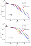Fig. 5. Gamma-ray spectrum for different choices of the parameters n and ${\widehat{l}}_c$. Panel a: Cases 1 to 3 of Table 1, all with n = 1. Panel b: Cases 4 to 6 (excluding Case 4b), with n = 0.9. The three curves on each panel correspond to different values of ${\widehat{l}}_c$, with $\widehat{Q}$ chosen so as to produce the same flux at Eγ = 1 TeV for all cases. The red dots are obtained from HESS Collaboration (2016).

The effect of the cutoff energy of the CR injection spectrum, E_max, is shown in Fig. 6. As expected, it causes the gamma-ray spectrum to cut off around E_γ ∼ κ_πE_max.

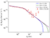Fig. 6. Gamma-ray spectrum for different maximum energies Emax = 1, 3, and 10 PeV (Cases 11, 2, and 12, respectively), all with the same parameter values n = 1, m = 0, q = 2, $\widehat{B}=1$, ${\widehat{l}}_c=3$, and slightly different values of $\widehat{Q}$, chosen so that the three spectra visually fit the H.E.S.S. data.

In Sect. 3.2, we use approximate expressions for Φ_γ(E_γ) (Eqs. 30 and 31) to argue that the exponent m of the radial profile of the coherence length l_c should not significantly affect the spectral index of the gamma-ray spectrum at low or high energies (α_LE and α_HE, respectively) or the gamma-ray energy that separates these two power-law regimes (E_γ ∼ 3 TeV). This is largely confirmed by Fig. 7a, which compares spectra for different values of m in the case n = 1. However, Eq. (31) implies that, in the case where n = 0.9, increasing the parameter m can weakly increase the index α_HE of the high-energy emission, making this part of the spectrum steeper. This is indeed what is seen in Fig. 7b, where only the case where m = 0.4 shows a noticeably steeper spectrum. However, we show in Sect. 4 that the self-consistency of our model requires m to be small (≲0.3), and so we do not expect any significant effect of the parameter m as long as this restriction is met.

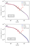Fig. 7. Dependence of the gamma-ray spectrum on the exponent m of the coherence length profile. Panel a: n = 1, ${\widehat{l}}_c=3,$m = 0, 0.2, 0.4 (Cases 2, 7 and 8 in Table 1). Panel b: n = 0.9, ${\widehat{l}}_c\approx 1,$m = 0, 0.2, 0.4 (Cases 4, 9 and 10).

Our findings therefore shows that models with $\widehat{B}=1$, q = 2, and E_max ≳ 1 PeV can accurately reproduce the main features of the spectrum of HESS J1745−290, including its break at E_γ, b ≈ 3 TeV. This happens for a narrow range of parameters spanned by the cases with n ≈ 1, ${\widehat{l}}_c\approx 3$, and $\widehat{Q}\approx 13$ on the one hand, and n ≈ 0.9, ${\widehat{l}}_c\approx 1$, and $\widehat{Q}\approx 6$ on the other. Remarkably, these values of q, $\widehat{Q}$, and E_max are in good agreement with the estimates from the diffuse CMZ emission, in particular those obtained by HESS Collaboration (2016). Regarding m, its effect on the spectrum is relatively weak, and it only appears at E_γ ≳ E_γ, b. These results, however, establish a strong restriction on the largely unknown parameter ${\widehat{l}}_c$, which needs to be in the range ${\widehat{l}}_c\approx 1-3$ (equivalent to a coherence length of l_c ≈ (1 − 3)×10¹⁴ cm).

4. Consistency

In this section we check the consistency of several simplifying assumptions made in the calculation of the gamma-ray emission.

4.1. Gas-density profile n_gas(r) for 0.07 pc < r< 0.4 pc.

According to Fig. 11 of Ressler et al. 2018, the n_gas(r) profile at 0.07pc ≲ r ≲ 0.4pc is steeper than the n_gas(r)∝r⁻¹ profile assumed in our calculations (Eq. 18). This means that our calculated gamma-ray emission is somewhat larger than what we would obtain if a more accurate profile were assumed.

Here we show that using Eq. 18 to model n_gas(r) in the range 0.07pc < r < 0.4pc only leads to a ∼20 − 30% overestimate in the emission and therefore does not affect significantly our results. This is shown in Fig. 3, where the purple dashed line represents the emission from 0.07pc < r < 0.4pc in our Case 2. We see that this emission is ≲20 − 30% of the total emission at all the energies of interest. Thus, assuming n_gas(r)∝r⁻¹ at all radii r < 0.4 pc should not significantly affect our main results.

4.2. Cosmic-ray transport for radii r > 0.4 pc

Even though CR transport at radii r > 0.4 pc is expected to be a combination of advection and diffusion, in our calculations we simply assume that transport at r > 0.4 pc is the same as at r = 0.4 pc. This should lead to an overestimate of the CR density in this region (as the assumed transport process may not be the most efficient one) and therefore provides an upper limit to its corresponding emission from r > 0.4 pc. In Fig. 3, the purple line represents this upper limit to the gamma-ray emission from r > 0.4 pc. We see that this emission is ≲3% of the total emission for all the energies of interest, and so this overestimate should not affect the accuracy of our results.

4.3. Validity of diffusion at r < 0.07 pc

In our calculations, we assume that diffusion is the dominant process for CR transport between r = r_min ∼ 10 R_g (where we expect the CRs to be injected) and r = 0.07 pc. In particular, at r ∼ 10 R_g, diffusion in the LED regime is assumed for CRs of all energies (as seen in the two cases (Case 2 and Case 4b) shown in Fig. 1). However, diffusive transport is a valid approximation for CR propagation only when r ≫ r_λ, where r_λ is defined as the radius where the CRs’ mean free path is equal to the radius itself, that is,

$$\begin{array}{c}\hfill r_{\lambda }={\lambda }_{\mathrm{mfp}}(r_{\lambda }).\end{array}$$(32)

From Eq. (16), we can obtain the expression for the mean free path of the CRs in the LED regime and show that r_λ satisfies

$$\begin{array}{c}\hfill \begin{array}{cc}\hfill {\left(\frac{r_{\lambda }}{10R_g}\right)}^{1-\frac{1}{3}(n+2m)}=& 6\times {10}^{-2}{(2.1\times {10}^4)}^{-2m/3}{\widehat{l}}_c^{2/3}{\widehat{B}}^{-1/3}{\left(\frac{E}{1\mathrm{TeV}}\right)}^{1/3}.\hfill \\ \hfill \end{array}\end{array}$$(33)

As the right hand side of Eq. (33) is a growing function of E, its upper limit is obtained by evaluating it at the maximum CR energy considered in this work, E = 10 PeV. This way we see that r_λ/(10 R_g) is always ≲2.7, implying that assuming diffusion in the LED regime is a valid approximation for r larger than ∼30R_g, which is just outside the region where CRs are injected in our model.

We note, however, that applying Eq. (33) to values of r_λ of as small as r ∼ 10 R_g may not be entirely consistent with the fact that Eq. (15) predicts the existence of a radius r_eq defined by

$$\begin{array}{c}\hfill r_{\mathrm{eq}}=l_c(r_{\mathrm{eq}}),\end{array}$$(34)

such that, at r ≲ r_eq, Eq. (15) is no longer a valid description of l_c(r) (because l_c(r) cannot be larger than r). Also, at r < r_eq, the diffusion process should behave more as a 1D process, in the sense that the propagation occurs along a nearly homogeneous background magnetic field. Therefore, in obtaining Eq. (33), we are implicitly making the simplifying assumption that the dependence of the CR mean free path on r at r < r_eq is the same as for r > r_eq. Given that this simplification only applies to r between ∼10R_g (∼10¹³ cm) and r_eq (≲10¹⁴ cm for ${\widehat{l}}_c\sim 1$), whereas most of the emission comes from large radii, we believe that it should not significantly affect the accuracy of our results.

4.4. Neglecting advection for r < 0.07 pc

In addition to influencing diffusion, advection can also contribute to CR transport because of the average radial gas velocity v_gas at r < 0.07 pc. Ressler et al. (2018) show that for 0.01 pc ≲ r ≲ 0.07 pc, there is a stagnation region where the mass-accretion rate averaged over the whole solid angle approaches Ṁ ≈ 0, indicating that v_gas should have a small effect on the CR transport in that region. In addition, for r ≲ 0.01 pc there is an inflow-dominated region where Ṁ is nearly constant. Taking Ṁ ≈ 10⁻⁸ M_⊙/year near the black hole (Dexter et al. 2020), we obtain the expression for v_gas given by Eq. (19). In order to neglect the effect of v_gas on the transport of the CRs, its magnitude has to be smaller than v_diff for the lowest-energy CRs, which diffuse in the LED regime for all radii r < 0.07 pc (as seen in Fig. 1). Considering the definition of v_diff from Eq. (9), we obtain:

$$\begin{array}{c}\hfill \begin{array}{cc}\hfill v_{\mathrm{diff}}\approx & 3\times {10}^{6}0.{52}^{2m}14.4^{n-1}{\widehat{l}}_c^{2/3}{\widehat{B}}^{-1/3}\hfill \\ \hfill & \times {\left(\frac{E}{\mathrm{TeV}}\right)}^{1/3}{\left(\frac{r}{0.01\mathrm{pc}}\right)}^{\frac{1}{3}(n+2m)-1}\mathrm{cm}/\mathrm{s},\hfill \end{array}\end{array}$$(35)

from which we obtain that the ratio v_diff/|v_gas| is

$$\begin{array}{c}\hfill \begin{array}{cc}\hfill \frac{v_{\mathrm{diff}}}{|v_{\mathrm{gas}}|}\approx & 90·0.{52}^{2m}14.4^{n-1}{\widehat{l}}_c^{2/3}{\widehat{B}}^{-1/3}{\left(\frac{E}{\mathrm{TeV}}\right)}^{1/3}\hfill \\ \hfill & \times {\left(\frac{r}{0.01\mathrm{pc}}\right)}^{\frac{1}{3}(n+2m)}.\hfill \end{array}\end{array}$$(36)

As we are focusing on emission with E_γ ≳ 0.2 TeV, the lowest CR energy that we consider is E ∼ 0.2/κ_π TeV ≈1 TeV. Therefore, since the ratio v_diff/|v_gas| is an increasing function of r, neglecting advection requires v_diff/|v_gas|≳1 for E = 1 TeV and r = 10R_g.

Figure 8a shows v_diff/|v_gas| as a function of m for E = 1 TeV and r = 10R_g, for the two favored cases in this work: n = 1, ${\widehat{l}}_c=3$, and n = 0.9, ${\widehat{l}}_c=1$, shown in blue and red, respectively. We see that for n = 1, ${\widehat{l}}_c=3$, neglecting advection requires m ≲ 0.4, while for n = 0.9, ${\widehat{l}}_c=1$, it requires m ≲ 0.3. This result shows that the consistency of our calculations demands a weak dependence of l_c on r, as assumed throughout this work.

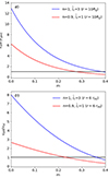Fig. 8. Panel a shows vdiff/|vgas| (Eq. (36)) as a function of m for E = 1 TeV and r = 10Rg. Panel b shows vdiff/vtd (Eq. (39)) as a function of m for E = 1 TeV and r = 6req. In both panels, the blue line represents the case n = 1, ${\widehat{l}}_c=3$, and the red line corresponds to n = 0.9, ${\widehat{l}}_c=1$, both with $\widehat{B}=1$.

Interestingly, the dependence of v_diff/|v_gas| on E also implies that, in our model, CRs of energies E≪ 1 TeV are significantly affected by advection towards the black hole, in principle not being able to propagate beyond r ∼ 10R_g. This implies that a significant fraction of these particles should simply be accreted onto the black hole, with their gamma-ray emission for E_γ ≪ κ_π × 1TeV ∼ 0.2 TeV not being captured by our model.

Cosmic rays could also be advected by the random motions of the MHD turbulence in the accretion flow, which we neglect in our model. If we estimate this turbulent velocity from the Alfvén velocity of the gas, ${\mathit{v}}_A=B/\sqrt{4\pi n_{\mathrm{gas}}{m}_p},$ and its length scale from l_c, the motion of the turbulence eddies should induce a CR diffusion characterized by a turbulent diffusion coefficient D_t given by

$$\begin{array}{c}\hfill D_t\sim l_c{v}_A/3,\end{array}$$(37)

which allows us to estimate a turbulent diffusion velocity, v_td, as

$$\begin{array}{c}\hfill v_{\mathit{td}}=D_t/r.\end{array}$$(38)

Combining Eqs. (13), (15), (18), (35), (37), and (38), one can show that

$$\begin{array}{c}\hfill \begin{array}{cc}\hfill \frac{v_{\mathrm{diff}}}{v_{\mathit{td}}}\approx & 120{(1.9)}^m{(43200)}^{n-1}{\widehat{l}}_c^{-\frac{1}{3}}{\widehat{B}}^{-\frac{4}{3}}{\left(\frac{E}{\mathrm{TeV}}\right)}^{\frac{1}{3}}\hfill \\ \hfill & \times {\left(\frac{r}{0.01\mathrm{pc}}\right)}^{\frac{4}{3}n-\frac{1}{3}m-\frac{1}{2}},\hfill \end{array}\end{array}$$(39)

which, for the values of n and m of interest (n ≈ 1 and m ≪ 1) is a growing function of r. Figure 8b shows v_diff/v_td as a function of m in the case where r = 6 r_eq, where r_eq is defined by Eq. (34), and for the smallest relevant energy E = 1 TeV. We can see that, in the cases of interest shown in the figure, v_diff/v_td ≳ 1 as long as m ≲ 0.3, which also satisfies the conditions for neglecting the effect of v_gas. Thus, as v_diff/v_td is a growing function of r, v_td can be safely neglected for r ≳ 6 r_eq. On the other hand, the effect of turbulent diffusion should be valid only for r ≳ r_eq. This means that there is a range of radii, r_eq ≲ r ≲ 6 r_eq, in which turbulent diffusion can contribute significantly to CR transport, implying that the CR density dn_CR/dE in that region should be somewhat smaller than what is obtained in our model. In order to find an upper limit to this effect, Figure 9 compares gamma-ray spectra calculated with r_min = 10 R_g and with r_min = 6 r_eq, otherwise with the same parameters. We see that there are only small differences (at E_γ ≳ 100 TeV) between the calculations with r_min = R_g and r_min = 6 r_eq, implying that neglecting turbulent diffusion should not significantly affect the accuracy of our results.

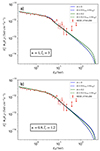Fig. 9. Effect of using different minimum radii rmin on the gamma-ray spectra. The solid and dashed lines represent analogous cases using rmin = 10 Rg and rmin = 6 req, respectively. Panels a and b show the cases where n = 1, ${\widehat{l}}_c=3$ and n = 0.9, ${\widehat{l}}_c=3$, respectively. In both panels we consider m = 0 (blue lines) and m = 0.2 (green lines).

This finding also reinforces the idea that gamma-ray emission is mainly produced at large radii, either close to 0.07 pc for E_γ ≲ 3 TeV or close to r_C(E_γ/κ_π) for E_γ ≳ 3 TeV, as shown in Fig 2.

4.5. Cosmic-ray, gas, and magnetic pressures

Our calculations assume that the gas properties in the accretion flow are determined by the hydrodynamic evolution of the wind of ∼30 WR stars that feed Sgr A*, as in the simulations of Ressler et al. (2018, 2020a) on which our results are based. However, the presence of CRs diffusing out from the central black hole can be dynamically important in this evolution if the CR pressure becomes comparable to the gas pressure. Figure 10 shows these two pressures as functions of r for the Cases 2 and 4b in Table 1 (corresponding to our fiducial cases with n = 1 and n = 0.9 shown in Fig. 1). The CR pressure is calculated as

$$\begin{array}{c}\hfill P_{\mathrm{CR}}r)=\frac{1}{3}{\displaystyle {\int }_{E_{\min }}^{E_{\max }}}\mathrm{d}EE\frac{\mathrm{d}{n}_{\mathrm{CR}}(E,r)}{\mathrm{d}E},\end{array}$$(40)

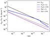Fig. 10. Cosmic-ray, gas and magnetic pressure comparison (PCR, Pgas and PB, respectively). The values of the parameters considered correspond to cases 2 (solid lines) and 4b (dashed lines) in Table 1.

where E_min = 1 TeV (as the CR density should be significantly suppressed for E ≪ 1 TeV, as shown in Sect. 4.4), and E_max = 3 PeV, while the gas pressure is calculated as

$$\begin{array}{c}\hfill P_{\mathrm{gas}}(r)=2n_{\mathrm{gas}}(r)k_B{T}_{\mathrm{gas}}(r),\end{array}$$(41)

where k_B is the Boltzmann constant, n_gas(r) is the gas density specified in Eq. (18), and T_gas(r) is the angle- and time-averaged temperature of the gas obtained from Fig. 11 of Ressler et al. (2018),⁶ as

$$\begin{array}{c}\hfill T_{\mathrm{gas}}(r)=1.5\times {10}^7{\left(\frac{r}{0.4\mathrm{pc}}\right)}^{-1}\mathrm{K}.\end{array}$$(42)

For completeness, we have also added the magnetic pressure profile for Cases 2 and 4b. We see that the gas pressure is dominant at almost all radii, with the CR pressure becoming relevant at r ∼ 0.07 pc, around the inner boundary of the region where the WR star winds feed the accretion flow (∼0.1 − 1 pc). The fact that P_CR and P_gas are comparable at r ∼ 0.07 pc may somewhat modify the evolution of the accreting gas near the feeding region. However, regarding the hydrodynamic properties of the gas, we use the fact that P_CR should only change the gas pressure by a factor ∼2 near r ∼ 0.07 pc, and thus assume that the gas dynamics at those radii is fairly well described by hydrodynamic considerations.

5. Diffusion timescales

The timescale for diffusion from the central black hole to a certain radius r can be estimated as t_diff ∼ r²/D(r) (valid as long as D(r) grows more slowly than r²). Above, we show that for CR energies E < E_C ∼ 20 TeV, most of the emission occurs close to the radius r ≈ 0.07 pc where the transition from the LED to the advection regime occurs. Therefore, the time for CRs to diffuse out and produce the gamma-ray emission below the break energy is

$$\begin{array}{c}\hfill \begin{array}{cc}\hfill t_{\mathrm{diff}}(E<E_C)& \sim \frac{{(0.07\mathrm{pc})}^2}{D_{\mathrm{LED}}(r=0.07\mathrm{pc})}\hfill \\ \hfill & \approx {10}^4{(2.1\times {10}^4)}^{\frac{1-n}{3}}{\widehat{l}}_c^{-\frac{2}{3}}{\widehat{B}}^{\frac{1}{3}}{\left(\frac{E}{\mathrm{TeV}}\right)}^{-\frac{1}{3}}\mathrm{yr}.\hfill \end{array}\end{array}$$(43)

On the other hand, for E > E_C, most of the emission occurs near the transition radius r_C(E) from the LED to the HED regime, for which the diffusion time is found to be

$$\begin{array}{c}\hfill \begin{array}{cc}\hfill t_{\mathrm{diff}}(E>E_C)& \sim \frac{{(r_C(E))}^2}{D_{\mathrm{LED}}(r_C(E))}\hfill \\ \hfill & \approx 1.7\times {10}^5{(5.7)}^{\frac{2-2n+m}{n-m}}{(2.1\times {10}^4)}^{\frac{(1-n)(1-m)}{n-m}}{\widehat{l}}_c^{\frac{2-n}{n-m}}{\widehat{B}}^{\frac{2-m}{n-m}}\hfill \\ \hfill & \times {\left(\frac{E}{\mathrm{TeV}}\right)}^{-\frac{2-m}{n-m}}\mathrm{yr}.\hfill \end{array}\end{array}$$(44)

For any given gamma-ray energy E_γ, the emission currently observed roughly averages over the injection rate of CRs of energy E ∼ E_γ/κ_π over the last t_diff(E). As expected, for all relevant energies, these diffusion times are much shorter than those corresponding to the CMZ, and therefore the gamma-ray emission of the point source is sensitive to much more recent activity (or inactivity) of the central black hole than the diffuse emission. Thus, the injection rate inferred from the point-source emission must not necessarily be the same as that explaining the CMZ; although we find them to be consistent with each other (with sizeable error bars on both).

It can also be seen from Eq. 44 that, for E > E_C, t_diff is a quickly decreasing function of E, mostly because of the decreasing critical radius r_C(E) (Eq. 25), which in turn is due to the rapidly increasing diffusion coefficient in the HED regime. For parameter choices favored by our model (n = 1, m = 0, ${\widehat{l}}_c=3$, $\widehat{B}=1$), we obtain t_diff ∼ 0.5 yr(E/PeV)⁻². Therefore, if the CR injection rate at PeV energies varies significantly on a comparable timescale (i.e., of the order of a few months), as suggested by the enhanced activity of Sgr A* in the radio, near-infrared, and X-ray bands during 2019 (Weldon et al. 2023 and references therein), this should be reflected in a significant variation of the gamma-ray emission at E_γ ≳ 100 TeV. This variable gamma-ray emission might be detectable in the near future by the Cherenkov Telescope Array Observatory (CTAO; Cherenkov Telescope Array Consortium 2019; Viana et al. 2019).

6. Conclusions

The spatial distribution of the diffuse gamma-ray emission detected in the CMZ (corresponding to the inner ∼100 pc of the Milky Way), along with its extended spectrum reaching ∼100 TeV energies, suggests the presence in the Galactic center of a “PeVatron”, that is, a CR accelerator capable of reaching PeV energies, which has been associated to the supermassive black hole Sgr A* (HESS Collaboration 2016). In addition, due to the apparently coincident position of the point-like gamma-ray source HESS J1745−290 with Sgr A*, a PeVatron could potentially allow an explanation of both the diffuse CMZ emission and the point source as being due to the same CRs accelerated in the immediate vicinity of Sgr A* and diffusing outwards from it. This scenario, however, is challenged by the fact that the spectrum of the point source shows a power-law behavior with a spectral turnover at a few TeV, which is not shown by the diffuse emission in the CMZ. Although this turnover is usually characterized as an exponential cutoff, the spectrum of the point source is also compatible with a broken power law (Aharonian et al. 2009; Adams et al. 2021), as we also show in Appendix A using observations from HESS Collaboration (2016).

In order to reconcile the CMZ and point source spectra, we propose a model for the point source in which the CRs are continuously injected near Sgr A* (within a radius r ∼ 10R_g) and subsequently diffuse through its accretion flow (r ≲ 0.1 pc). This way, very high-energy gamma rays are emitted in the accretion flow via inelastic hadronic collisions between the CR protons and the background protons. A key feature of this model is the existence of two CR diffusion regimes within the accretion flow of Sgr A*. These regimes, according to theoretical arguments and test-particle simulations of CR propagation in synthetic MHD turbulence (which we assume is strong and has a Kolmogorov spectrum), depend on the ratio between the Larmor radius, R_L, of the CRs and the coherence length, l_c, of the turbulence. This way, the transition between these two regimes gives rise to a significant depletion of the highest-energy CRs (R_L/l_c ≫ 1) within the emission region, which explains the existence of a break in the point-source spectrum.

The free parameters of our model characterize the spectrum of the injected CRs, their propagation efficiency through the accretion flow, and the properties of the background gas. Interestingly, the values of these parameters, which are required to fit HESS J1745-290, are all consistent with expectations from the observations of the diffuse emission from the CMZ and with previous hydrodynamical and MHD simulations of the Sgr A* accretion flow. The only exception is given by the (very uncertain) coherence length of the magnetic turbulence, which needs to have an approximately homogeneous value, l_c ∼ (1 − 3)×10¹⁴ cm ≈ (3 × 10⁻⁵ − 10⁻⁴) pc. Although disentangling the possible origin of this rather small coherence length is beyond the scope of this work, we speculate that its value might be affected by various processes, such as hydrodynamic instabilities in the colliding winds of the WR stars (Calderón et al. 2020) or even MHD instabilities driven by the CRs themselves. Indeed, in Sect. 4.5 we show that the CR pressure can be dynamically important within the feeding region (0.07 pc ≲ r ≲ 0.4 pc), where gas injection from the WR stars occurs. This region thus appears as an ideal environment for the action of, for example, the nonresonant instability, which is driven by the electric current of the CRs and has the potential to produce highly nonlinear MHD turbulence (Bell 2004, 2005; Riquelme & Spitkovsky 2009, 2010). We defer the study of these possible sources of turbulence to future research.

Our results therefore support the hypothesis that Sgr A* is capable of accelerating CRs up to a few PeV, contributing to explaining the origin of Galactic CRs up to the “knee”. It is worth emphasizing, however, that although we define our CR acceleration region very close to Sgr A* (at r ∼ 10R_g), the obtained emission spectra from our model are highly insensitive to the precise location of the injection region, as long as this region is anywhere in the range r ∼ (10 − 10³) R_g (see discussion in Sect. 3.1).

Our model has the potential to be tested by future TeV telescopes, such as CTAO (Cherenkov Telescope Array Consortium 2019). Given the small size of the emitting region (r ≲ 0.1 pc, equivalent to ≲3 arcsec in angular size), our model predicts a gamma-ray source that cannot be resolved by any foreseeable TeV observatory. However, an interesting prediction of our model is that the spectrum of the point source should be a broken power law, with specific spectral indices α_LE ≈ 2.3 for E_γ ≲ 3 TeV and α_HE ≈ 3 for E_γ ≳ 3 TeV (see discussion in Sect. 3.2). This is in contrast to a single power law with an exponential cutoff, as has been suggested by other models (e.g., Guo et al. 2017). This means that, at gamma-ray energies of ≳ 10 TeV, the gamma-ray spectrum obtained from our model becomes notably different from other competing models. This is particularly interesting given that CTAO will be approximatelly ten times more sensitive than H.E.S.S., thus allowing us, in principle, to discriminate between the different models. Further model discrimination might be done using the possible time variability of HESS J1745−290 at the highest energies. This is interesting given the significant variability exhibited by Sgr A* at various wavelengths. Although our model assumes a steady injection of CRs, in Sect. 5 we estimate that, if CR injection were variable, our model would predict potentially significant variability at E_γ ∼ 100 TeV on timescales of as short as months. To date, however, observations have failed to detect variability of the HESS J1745−290 gamma-ray point source, possibly because current observatories do not possess the required sensitivity to detect such variability. In this respect, the upcoming observations with CTAO may, in principle, have sufficiently sensitivity to detect the point-source variability. We defer the study of this possibility to future research.

Acknowledgments

The authors gratefully acknowledge support from ANID-FONDECYT grants 1191673 and 1201582, as well as the Center for Astrophysics and Associated Technologies (CATA; ANID Basal grant FB210003).

References

Appendix A: Fitting HESS J1745-290 spectrum with a broken power law

The central point source HESS J1745-290 is usually characterized by a hard power law spectrum with a photon index ∼2.1 and an exponential cutoff at ∼10 TeV. When compared with a pure power law, the power law with an exponential cutoff (ECPL) is clearly preferred by the data (HESS Collaboration 2016).

Besides a power law with an exponential cutoff, the spectral shape of HESS J1745-290 has also been shown to be compatible with a broken power law with the break energy at a few TeV (Aharonian et al. 2009; Adams et al. 2021). Here we use more up-to-date H.E.S.S. observations of this source obtained from HESS Collaboration (2016) to confirm this point.

Fig. A.1 shows two least-squares fits of the point source (for which we used the Levenberg-Marquardt algorithm). The blue line corresponds to a broken power-law (BPL) model for the photon flux, Φ_γ(E_γ), given by

$$\begin{array}{c}\hfill {\mathrm{\Phi }}_{\gamma }(E_{\gamma })=\frac{{\mathrm{\Phi }}_0{(E_{\gamma }/E_c)}^{-{\mathrm{\Gamma }}_1}}{1+{(E_{\gamma }/E_c)}^{{\mathrm{\Gamma }}_2-{\mathrm{\Gamma }}_1}},\end{array}$$(A.1)

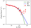Fig. A.1. Least squares fits of the point source spectrum. The blue and green lines correspond to a BPL model and a single ECPL model for photon fluxes given by Eqs. A.1 and A.2, respectively. The red circles correspond to H.E.S.S. data from HESS Collaboration (2016).

for which we obtain Φ₀ = (2.44 ± 1.2)×10⁻¹⁴ TeV⁻¹ cm⁻² s⁻¹, E_c = 8.22 ± 1.4 TeV, Γ₁ = 2.18 ± 0.04, Γ₂ = 3.89 ± 0.52, a p-value of p = 0.63, and χ²/DOF = 0.87.

The green line corresponds to a ECPL model given by

$$\begin{array}{c}\hfill {\mathrm{\Phi }}_{\gamma }(E_{\gamma })={\mathrm{\Phi }}_0{(E_{\gamma }/E_c)}^{-{\mathrm{\Gamma }}_1}{e}^{-E_{\gamma }/E_c},\end{array}$$(A.2)

for which we find Φ₀ = (1.83 ± 0.88)×10⁻¹⁴ TeV⁻¹ cm⁻² s⁻¹, E_c = 10.13 ± 1.89 TeV, Γ₁ = 2.13 ± 0.03, a p-value of p = 0.62, and χ²/DOF = 0.88. The similar values of p and χ²/DOF obtained from these two fits imply that the BPL and ECPL models are both compatible with the current H.E.S.S. data from HESS Collaboration (2016).

Appendix B: Heuristic derivation of the diffusion coefficients

Here, we give simple, rough, physical derivations of the effective mean free paths, λ_mfp, and therefore of the diffusion coefficients, D = λ_mfpc/3, of relativistic, charged particles in a medium with isotropic, magnetic Kolmogorov turbulence with coherence length l_c and Larmor radius R_L. For the HED regime, R_L ≫ l_c, a similar derivation has been given by Subedi et al. (2017), and we give it here for completeness. For the LED regime, R_L ≪ l_c, we are not aware of a similar derivation in the literature. For simplicity and given the rough approximations involved, we generally ignore numerical factors ∼2π and smaller.

B.1. High-energy diffusion (HED) regime

If R_L ≫ l_c, as a particle crosses a coherence length l_c, it deviates only by a small angle, θ₁ ∼ l_c/R_L. These deviations are random, in different directions for successive steps of size l_c. Therefore, the direction of motion undergoes a random walk, accumulating a typical deviation ${\theta }_N\sim \sqrt{N}{\theta }_1$ after N such steps. The direction of motion will have changed significantly once θ_N ∼ 1, implying N ∼ (R_L/l_c)², which defines the mean free path ${\lambda }_{\text{mfp}}~N{l}_c~R_L^2/l_c$.

B.2. Low-energy diffusion (LED) regime

On scales ≪l_c, the magnetic field can be approximated by B = B₀ + δBr), where B₀ = constant and |δB(r)| ≪ B₀. If R_L ≡ γmc²/(qB₀)≪l_c, where γ, m, and q are the Lorentz factor, the mass, and the charge of the particles, respectively, the latter will follow a roughly helical motion, typically with velocity components of similar magnitude (not much smaller than c) along B₀, v_‖, and perpendicular to it, v_⊥. Thus, the particles will move a distance ∼R_L along B₀ while completing an orbit of radius ∼R_L in the perpendicular plane.

The equation of motion for the parallel velocity component is

$$\begin{array}{c}\hfill \gamma m\frac{\mathrm{d}{\mathit{v}}_{\Vert }}{\mathrm{d}t}=\frac{q}{c}{\mathit{v}}_{\perp }\times \delta \mathit{B}.\end{array}$$(B.1)

Since the direction of v_⊥ completes a loop while the particle travels a distance ∼R_L, v_‖ will be mostly affected by field perturbations on roughly the same scale, which we will call δB^*. Its typical change while traveling this scale will be small, Δv_∥, 1 ∼ cδB^*/B₀, but these random changes can accumulate, yielding a substantial change $\mathrm{\Delta }{\mathit{v}}_{\Vert ,N}\sim \sqrt{N}\mathrm{\Delta }{\mathit{v}}_{\Vert ,1}\sim c$ after N ∼ (c/Δv_∥, 1)² steps, corresponding to a one-dimensional mean free path (along B₀) given by λ_mfp ∼ R_L(B₀/δB^*)². For Kolmogorov turbulence, B₀/δB^* ∼ (l_c/R_L)^1/3, therefore the one-dimensional mean free path is

$$\begin{array}{c}\hfill {\lambda }_{\mathrm{mfp}}\sim R_L^{1/3}{l}_c^{2/3},\end{array}$$(B.2)

with a corresponding diffusion coefficient D_1D = λ_mfpc/3.

The time required to diffuse a distance l_c along B₀ is $t_c~l_c^2/D_{\text{1D}}$. On each patch of size l_c, the magnetic field has a random orientation. Thus, on larger scales, the diffusion process becomes three-dimensional, with steps of size l_c traversed at a typical speed v_c ∼ l_c/t_c, so the large-scale, three-dimensional diffusion coefficient is $D~l_c{v}_c/3~l_c^2/t_c~D_{\text{1D}}$, as in the one-dimensional analysis above.

Appendix C: Full expressions for dn_CR/dE

In this appendix we describe the analytical treatment for the CR density distribution per unit energy dn_CR/dE of our full model described in Sect. 2.

C.1. Continuity and boundary conditions

As explained in 2.1, in order to determine the CR density distribution on the Sgr A* accretion flow, we solve Eq. 8 neglecting one of the two terms on the right hand side, depending on whether diffusion of advection dominates. In the case dominated by diffusion, we have

$$\begin{array}{c}\hfill \frac{\mathrm{d}N}{\mathrm{d}E\mathrm{d}t}(E)=-4\pi r^{2}D(E,r)\frac{\partial }{\partial r}\left(\frac{\mathrm{d}{n}_{\mathrm{CR}}}{\mathrm{d}E}(E,r)\right),\end{array}$$(C.1)

while is advection is the dominant transport mechanism of CRs,

$$\begin{array}{c}\hfill \frac{\mathrm{d}N}{\mathrm{d}E\mathrm{d}t}(E)=4\pi r^2{v}_{\mathrm{gas}}(r)\frac{\mathrm{d}{n}_{\mathrm{CR}}}{\mathrm{d}E}(E,r).\end{array}$$(C.2)

The above equations for dn_CR/dE are constrained by continuity restrictions, which we characterize in Fig. C.1, noting that: r_C(E) represent the critical radius at which a CR of energy E will transit from the LED regime to HED regime (see Eq. 25), r_C, ad(E) represent the radius at which a CR of energy E transit from the HED regime to the AD regime (see Eq. 27), given that the gas velocity is determined by Eq. 20.

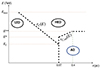Fig. C.1. Schematic representation of the different CR transport regimes used to calculate dnCR/dE, as a function of radius r and CR energy E. These regimes correspond to low-energy diffusion (LED), high-energy diffusion (HED) and advection-dominated (AD).

Fig C.1, shows a schematic representation of the different CR transport regimes used to calculate dn_CR/dE, as a function of radius r and CR energy E. We see that, besides E_C (defined by r_C(E) = 0.07 pc), the limits between these regions are characterized by the energies E^* and E^**, corresponding to the energies where r_C, ad(E) becomes equal to 0.07 pc and 0.4 pc, respectively. Thus, the continuity conditions for the CR density can be described within the four energy ranges shown in Fig C.1:

1. Energy range E ϵ [1TeV − E_C]:

   $$\begin{array}{c}\hfill \frac{d{n}_{\mathit{CR}}}{\mathit{dE}}{{|}_{\mathit{LED}}(E,r=0.07\mathrm{pc})=\frac{d{n}_{\mathit{CR}}}{\mathit{dE}}|}_{\mathit{AD}}(E,r=0.07\mathrm{pc}).\end{array}$$(C.3)

2. Energy range E ϵ [E_C − E^*]:

   $$\begin{array}{c}\hfill \frac{d{n}_{\mathit{CR}}}{\mathit{dE}}{{|}_{\mathit{LED}}(E,r=r_C(E))=\frac{d{n}_{\mathit{CR}}}{\mathit{dE}}|}_{\mathit{HED}}(E,r=r_C(E)),\mathrm{and}\end{array}$$(C.4)

   $$\begin{array}{c}\hfill \frac{d{n}_{\mathit{CR}}}{\mathit{dE}}{{|}_{\mathit{HED}}(E,r=0.07\mathrm{pc})=\frac{d{n}_{\mathit{CR}}}{\mathit{dE}}|}_{\mathit{AD}}(E,r=0.07\mathrm{pc}).\end{array}$$(C.5)

3. Energy range E ϵ [E^* − E^**]:

   $$\begin{array}{c}\hfill \frac{d{n}_{\mathit{CR}}}{\mathit{dE}}{{|}_{\mathit{LED}}(E,r=r_C(E))=\frac{d{n}_{\mathit{CR}}}{\mathit{dE}}|}_{\mathit{HED}}(E,r=r_C(E)),\mathrm{and}\end{array}$$(C.6)

   $$\begin{array}{c}\hfill \frac{d{n}_{\mathit{CR}}}{\mathit{dE}}{{|}_{\mathit{HED}}(E,r=r_{C,ad}(E))=\frac{d{n}_{\mathit{CR}}}{\mathit{dE}}|}_{\mathit{AD}}(E,r=r_{C,ad}(E))\end{array}$$(C.7)

4. Energy range E ϵ [E^** − E_max]:

   $$\begin{array}{c}\hfill \frac{d{n}_{\mathit{CR}}}{\mathit{dE}}{{|}_{\mathit{LED}}(E,r=r_C(E))=\frac{d{n}_{\mathit{CR}}}{\mathit{dE}}|}_{\mathit{HED}}(E,r=r_C(E)).\end{array}$$(C.8)

References

- Adams, C. B., Benbow, W., Brill, A., et al. 2021, ApJ, 913, 115 [NASA ADS] [CrossRef] [Google Scholar]
- Aharonian, F. 2004, Very High Energy Cosmic Gamma Radiation: a Crucial Window on the Extreme Universe (World Scientific) [CrossRef] [Google Scholar]
- Aharonian, F., & Neronov, A. 2005, Astrophys. Space Sci., 300, 255 [NASA ADS] [CrossRef] [Google Scholar]
- Aharonian, F., Akhperjanian, A. G., Aye, K. M., et al. 2004, A&A, 425, L13 [NASA ADS] [CrossRef] [EDP Sciences] [Google Scholar]
- Aharonian, F., Akhperjanian, A. G., Bazer-Bachi, A. R., et al. 2006, Phys. Rev. Lett., 97, 221102 [NASA ADS] [CrossRef] [Google Scholar]
- Aharonian, F., Akhperjanian, A. G., Anton, G., et al. 2009, A&A, 503, 817 [NASA ADS] [CrossRef] [EDP Sciences] [Google Scholar]
- Aharonian, F., Yang, R., & de Oña Wilhelmi, E. 2019, Nat. Astron., 3, 561 [Google Scholar]
- Albert, J., Aliu, E., Anderhub, H., et al. 2006, ApJ, 638, L101 [NASA ADS] [CrossRef] [Google Scholar]
- Aloisio, R., & Berezinsky, V. 2004, ApJ, 612, 900 [NASA ADS] [CrossRef] [Google Scholar]
- Bell, A. R. 2004, MNRAS, 353, 550 [Google Scholar]
- Bell, A. R. 2005, MNRAS, 358, 181 [NASA ADS] [CrossRef] [Google Scholar]
- Calderón, D., Cuadra, J., Schartmann, M., et al. 2020, MNRAS, 493, 447 [Google Scholar]
- Cembranos, J. A. R., Gammaldi, V., & Maroto, A. L. 2012, Phys. Rev. D, 86, 103506 [NASA ADS] [CrossRef] [Google Scholar]
- Cherenkov Telescope Array Consortium (Acharya, B. S., et al.) 2019, Science with the Cherenkov Telescope Array [Google Scholar]
- Chernyakova, M., Malyshev, D., Aharonian, F. A., Crocker, R. M., & Jones, D. I. 2011, ApJ, 726, 60 [NASA ADS] [CrossRef] [Google Scholar]
- Clavel, M., Terrier, R., Goldwurm, A., et al. 2013, A&A, 558, A32 [NASA ADS] [CrossRef] [EDP Sciences] [Google Scholar]
- Cuadra, J., Nayakshin, S., Springel, V., & Di Matteo, T. 2006, MNRAS, 366, 358 [NASA ADS] [CrossRef] [Google Scholar]
- Cuadra, J., Nayakshin, S., & Martins, F. 2007, MNRAS, 383, 458 [Google Scholar]
- Dexter, J., Jiménez-Rosales, A., Ressler, S. M., et al. 2020, MNRAS, 494, 4168 [NASA ADS] [CrossRef] [Google Scholar]
- Dörner, J., Becker Tjus, J., Blomenkamp, P. S., et al. 2024, ApJ, 965, 180 [CrossRef] [Google Scholar]
- Dundovic, A., Pezzi, O., Blasi, P., Evoli, C., & Matthaeus, W. H. 2020, Phys. Rev. D, 102, 103016 [NASA ADS] [CrossRef] [Google Scholar]
- Eatough, R. P., Falcke, H., Karuppusamy, R., et al. 2013, Nature, 501, 391 [Google Scholar]
- Fleishman, G. D., & Toptygin, I. N. 2013, Cosmic Electrodynamics: Electrodynamics and Magnetic Hydrodynamics of Cosmic Plasmas (Springer), 388 [CrossRef] [Google Scholar]
- Funk, S., & Hinton, J. A. 2008, Am. Inst. Phys. Conf. Ser., 1085, 882 [NASA ADS] [Google Scholar]
- GRAVITY Collaboration (Abuter, R., et al.) 2018, A&A, 618, L10 [NASA ADS] [CrossRef] [EDP Sciences] [Google Scholar]
- Guo, Y.-Q., Tian, Z., Wang, Z., Li, H.-J., & Chen, T.-L. 2017, ApJ, 836, 233 [NASA ADS] [CrossRef] [Google Scholar]
- HESS Collaboration (Abramowski, A., et al.) 2016, Nature, 531, 476 [Google Scholar]
- HESS Collaboration (Abdalla, H., et al.) 2018, A&A, 612, A9 [NASA ADS] [CrossRef] [EDP Sciences] [Google Scholar]
- Hinton, J. A., & Aharonian, F. A. 2007, ApJ, 657, 302 [NASA ADS] [CrossRef] [Google Scholar]
- Hooper, D., de la Calle Perez, I., Silk, J., Ferrer, F., & Sarkar, S. 2004, JCAP, 2004, 002 [CrossRef] [Google Scholar]
- Hosek, M. W., Do, T., Lu, J. R., et al. 2022, ApJ, 939, 68 [NASA ADS] [CrossRef] [Google Scholar]
- Kosack, K., Badran, H. M., Bond, I. H., et al. 2004, ApJ, 608, L97 [CrossRef] [Google Scholar]
- Liu, R.-Y., Wang, X.-Y., Prosekin, A., & Chang, X.-C. 2016, ApJ, 833, 200 [NASA ADS] [CrossRef] [Google Scholar]
- MAGIC Collaboration (Acciari, V. A., et al.) 2020, A&A, 642, A190 [NASA ADS] [CrossRef] [EDP Sciences] [Google Scholar]
- Marin, F., Churazov, E., Khabibullin, I., et al. 2023, Nature, 619, 41 [Google Scholar]
- Mertsch, P. 2020, Ap&SS, 365, 135 [NASA ADS] [CrossRef] [Google Scholar]
- Muno, M. P., Baganoff, F. K., Bautz, M. W., et al. 2004, ApJ, 613, 326 [NASA ADS] [CrossRef] [Google Scholar]
- Ponti, G., George, E., Scaringi, S., et al. 2017, MNRAS, 468, 2447 [NASA ADS] [CrossRef] [Google Scholar]
- Profumo, S. 2005, Phys. Rev. D, 72, 103521 [NASA ADS] [CrossRef] [Google Scholar]
- Reichherzer, P., Becker Tjus, J., Zweibel, E. G., Merten, L., & Pueschel, M. J. 2022a, MNRAS, 514, 2658 [NASA ADS] [CrossRef] [Google Scholar]
- Reichherzer, P., Merten, L., Dörner, J., et al. 2022b, SN Appl. Sci., 4, 15 [NASA ADS] [CrossRef] [Google Scholar]
- Reichherzer, P., Bott, A. F. A., Ewart, R. J., et al. 2023, ArXiv e-prints [arXiv:2311.01497] [Google Scholar]
- Ressler, S. M., Quataert, E., & Stone, J. M. 2018, MNRAS, 478, 3544 [NASA ADS] [CrossRef] [Google Scholar]
- Ressler, S. M., Quataert, E., & Stone, J. M. 2020a, MNRAS, 492, 3272 [NASA ADS] [CrossRef] [Google Scholar]
- Ressler, S. M., White, C. J., Quataert, E., & Stone, J. M. 2020b, ApJ, 896, L6 [NASA ADS] [CrossRef] [Google Scholar]
- Riquelme, M. A., & Spitkovsky, A. 2009, ApJ, 694, 626 [Google Scholar]
- Riquelme, M. A., & Spitkovsky, A. 2010, ApJ, 717, 1054 [CrossRef] [Google Scholar]
- Rodríguez-Ramírez, J. C., de Gouveia Dal Pino, E. M., & Alves Batista, R. 2019, ApJ, 879, 6 [Google Scholar]
- Scepi, N., Dexter, J., & Begelman, M. C. 2022, MNRAS, 511, 3536 [NASA ADS] [CrossRef] [Google Scholar]
- Scherer, A., Cuadra, J., & Bauer, F. E. 2022, A&A, 659, A105 [NASA ADS] [CrossRef] [EDP Sciences] [Google Scholar]
- Scherer, A., Cuadra, J., & Bauer, F. E. 2023, A&A, 679, A114 [NASA ADS] [CrossRef] [EDP Sciences] [Google Scholar]
- Strong, A. W., Moskalenko, I. V., & Ptuskin, V. S. 2007, Ann. Rev. Nucl. Part. Sci., 57, 285 [NASA ADS] [CrossRef] [Google Scholar]
- Su, M., Slatyer, T. R., & Finkbeiner, D. P. 2010, ApJ, 724, 1044 [Google Scholar]
- Subedi, P., Sonsrettee, W., Blasi, P., et al. 2017, ApJ, 837, 140 [Google Scholar]
- Subroweit, M., Mossoux, E., & Eckart, A. 2020, ApJ, 898, 138 [CrossRef] [Google Scholar]
- Tsuchiya, K., Enomoto, R., Ksenofontov, L. T., et al. 2004, ApJ, 606, L115 [CrossRef] [Google Scholar]
- Viana, A., Ventura, S., Gaggero, D., et al. 2019, Int. Cosmic Ray Conf., 36, 817 [NASA ADS] [CrossRef] [Google Scholar]
- Wang, Q. D., Lu, F. J., & Gotthelf, E. V. 2006, MNRAS, 367, 937 [NASA ADS] [CrossRef] [Google Scholar]
- Weldon, G. C., Do, T., Witzel, G., et al. 2023, ApJ, 954, L33 [NASA ADS] [CrossRef] [Google Scholar]
- Zhang, J. L., Bi, X. J., & Hu, H. B. 2006, A&A, 449, 641 [NASA ADS] [CrossRef] [EDP Sciences] [Google Scholar]