| Issue |
A&A
Volume 690, October 2024
|
|
|---|---|---|
| Article Number | A185 | |
| Number of page(s) | 16 | |
| Section | Stellar structure and evolution | |
| DOI | https://doi.org/10.1051/0004-6361/202449794 | |
| Published online | 08 October 2024 | |
Dynamical accretion flows
ALMAGAL: Flows along filamentary structures in high-mass star-forming clusters
1
Max-Planck-Institut für Astronomie, Königstuhl 17, 69117 Heidelberg, Germany
2
INAF-Istituto di Astrofisica e Planetologia Spaziale, Via Fosso del Cavaliere 100, 00133 Roma, Italy
3
I. Physikalisches Institut, Universität zu Köln, Zülpicher Str. 77, 50937 Köln, Germany
4
University of Connecticut, Department of Physics, 2152 Hillside Road, Unit 3046, Storrs, CT 06269, USA
5
Institute of Astronomy and Astrophysics, Academia Sinica, Taipei 10617, Taiwan
6
East Asian Observatory, 660 N. A’ohoku, Hilo, Hawaii, HI 96720, USA
7
Institut de Ciéncies de l’Espai (ICE, CSIC), Can Magrans s/n, 08193 Bellaterra, Barcelona, Spain
8
Institut d’Estudis Espacials de Catalunya (IEEC), Barcelona, Spain
9
Universität Heidelberg, Zentrum für Astronomie, Institut für Theoretische Astrophysik, Heidelberg, Germany
10
Universität Heidelberg, Interdisziplinäres Zentrum für Wissenschaftliches Rechnen, Heidelberg, Germany
11
Harvard-Smithsonian Center for Astrophysics, 160 Garden St, Cambridge, MA 02420, USA
12
Center for Data and Simulation Science, University of Cologne, Cologne, Germany
13
INAF – Osservatorio Astrofisico di Arcetri, Largo E. Fermi 5, 50125 Firenze, Italy
14
Jodrell Bank Centre for Astrophysics & UK ALMA Regional Centre Node, School of Physics & Astronomy, University of Manchester, Manchester M13 9PL, UK
15
Jet Propulsion Laboratory, California Institute of Technology, 4800 Oak Grove Drive, Pasadena, CA 91109, USA
16
SRON Netherlands Institute for Space Research, Landleven 12, 9747 AD Groningen, The Netherlands
17
Kapteyn Astronomical Institute, University of Groningen, Groningen, The Netherlands
18
UK Astronomy Technology Centre, Royal Observatory Edinburgh, Blackford Hill, Edinburgh EH9 3HJ, UK
19
National Radio Astronomy Observatory (NRAO), 520 Edgemont Rd, Charlottesville, VA 22903, USA
20
UK ALMA Regional Centre Node, Manchester M13 9PL, UK
21
SKA Observatory, Jodrell Bank, Lower Withington, Macclesfield SK11 9FT, UK
22
National Astronomical Observatory of Japan, National Institutes of Natural Sciences, 2-21-1 Osawa, Mitaka, Tokyo 181-8588, Japan
23
Department of Astronomical Science, SOKENDAI (The Graduate University for Advanced Studies), 2-21-1 Osawa, Mitaka, Tokyo 181-8588, Japan
24
Dipartimento di Fisica, Universita di Roma La Sapienza, Piazzale Aldo Moro 2, 00185 Roma, Italy
25
Faculty of Physics, University of Duisburg-Essen, Duisburg, Germany
26
Shanghai Astronomical Observatory, Chinese Academy of Sciences, 80 Nandan Road, Shanghai 200030, PR China
27
Centre for Astrochemical Studies, Max-Planck-Institute for Extraterrestrial Physics, Giessenbachstrasse 1, 85748 Garching, Germany
28
LERMA, Observatoire de Paris, PSL Research University, CNRS, Sorbonne Universite, 92190 Meudon, France
29
INAF-Istituto di Radioastronomia & Italian ALMA Regional Centre, Via P. Gobetti 101, 40129 Bologna, Italy
30
Max-Planck-Institut fur Radioastronomie (MPIfR), Auf dem Hügel 69, 53121 Bonn, Germany
31
Department of Astrophysical and Planetary Sciences, University of Colorado, Boulder, CO 80389, USA
32
Leiden Observatory, Leiden University, PO Box 9513 2300 RA Leiden, The Netherlands
33
Departamento de Astronomía, Universidad de Chile, Santiago, Chile
34
European Southern Observatory, Karl-Schwarzschild-Strasse 2, 85748 Garching, Germany
35
Department of Space, Earth & Environment, Chalmers University of Technology, 412 96 Gothenburg, Sweden
36
Dipartimento di Fisica e Astronomia “Augusto Righi”, Viale Berti Pichat 6/2, Bologna, Italy
37
Universidad Autónoma de Chile, Nucleo Astroquimica y Astrofisica, Avda Pedro de Valdivia 425, Providencia, Santiago de Chile, Chile
38
Max Planck Institute for Extraterrestrial Physics, Giessenbachstraße 1, 85749 Garching bei München, Germany
39
School of Physics and Astronomy, University of Leeds, Leeds LS2 9JT, UK
⋆ Corresponding author; This email address is being protected from spambots. You need JavaScript enabled to view it.
.
Received:
29
February
2024
Accepted:
7
August
2024
Abstract
Context. Investigating the flow of material along filamentary structures towards the central core can help provide insights into high-mass star formation and evolution.
Aims. Our main motivation is to answer the question of what the properties of accretion flows are in star-forming clusters. We used data from the ALMA Evolutionary Study of High Mass Protocluster Formation in the Galaxy (ALMAGAL) survey to study 100 ALMAGAL regions at a ∼1″ resolution, located between ∼2 and 6 kpc.
Methods. Making use of the ALMAGAL ∼1.3 mm line and continuum data, we estimated flow rates onto individual cores. We focus specifically on flow rates along filamentary structures associated with these cores. Our primary analysis is centered around position velocity cuts in H2CO (30, 3–20, 2), which allow us to measure the velocity fields surrounding these cores. Combining this work with column density estimates, we were able to derive the flow rates along the extended filamentary structures associated with cores in these regions.
Results. We selected a sample of 100 ALMAGAL regions, covering four evolutionary stages from quiescent to protostellar, young stellar objects (YSOs), and HII regions (25 each). Using a dendrogram and line analysis, we identify a final sample of 182 cores in 87 regions. In this paper, we present 728 flow rates for our sample (4 per core), analysed in the context of evolutionary stage, distance from the core, and core mass. On average, for the whole sample, we derived flow rates on the order of ∼10−4 M⊙ yr−1 with estimated uncertainties of ±50%. We see increasing differences in the values among evolutionary stages, most notably between the less evolved (quiescent and protostellar) and more evolved (YSO and HII region) sources and we also see an increasing trend as we move further away from the centre of these cores. We also find a clear relationship between the calculated flow rates and core masses ∼M2/3, which is in line with the result expected from the tidal-lobe accretion mechanism. The significance of these relationships is tested with Kolmogorov–Smirnov and Mann-Whitney U tests.
Conclusions. Overall, we see an increasing trend in the relationships between the flow rate and the three investigated parameters, namely: evolutionary stage, distance from the core, and core mass.
Key words: accretion, accretion disks / stars: evolution / stars: massive
© The Authors 2024
 Open Access article, published by EDP Sciences, under the terms of the Creative Commons Attribution License (https://creativecommons.org/licenses/by/4.0), which permits unrestricted use, distribution, and reproduction in any medium, provided the original work is properly cited.
This article is published in open access under the Subscribe-to-Open model.
Open access funding provided by Max Planck Society.
1. Introduction
The formation and evolution of high-mass stars have been the subject of intense scientific interest for decades. High-mass stars play a crucial role in shaping not only their parental clouds, but also the interstellar medium on kpc scales, enriching it with heavy elements and influencing the dynamics of their surrounding environments via the energy they release through radiation and stellar winds (e.g., Kahn 1974; Yorke & Kruegel 1977; Wolfire & Cassinelli 1987; Zinnecker & Yorke 2007; Arce et al. 2007; Frank et al. 2014; Smith et al. 2009; Zhang et al. 2015; Motte et al. 2018; Kuiper & Hosokawa 2018). This, in turn, triggers new waves of star formation and helps sculpt the physical conditions of the interstellar medium (ISM) in galactic disks. Therefore, understanding the intricate processes involved in the birth and subsequent evolution of high-mass stars is fundamental not only for stellar physics, but also for comprehending the broader aspects of galaxy formation and evolution. High-mass stars are rare due to their short lifetimes and comparatively low numbers when compared to low-mass stars. Looking at the initial mass function (IMF), we see one reason they are in limited numbers is that the IMF at high mass values follows a power law (e.g., Salpeter 1955; Bonnell et al. 2007; Offner et al. 2014). Moreover, high-mass stars typically stay embedded in their natal clusters until they reach the main sequence, making it much more difficult for us to study and constrain how they form and evolve. This leaves us with a large knowledge gap in not only star formation, but astrophysics in general.
What we do know is that the most common place for star formation to occur is in clustered environments inside giant molecular clouds (GMCs, e.g., Lada & Lada 2003; Bressert et al. 2010). These are immense reservoirs of cold, dense gas and dust that provide the material for new generations of stars. Molecular clouds are commonly described to have a hierarchical structure (e.g., Scalo 1985; Thomasson et al. 2022). Following Williams et al. (2000) and Beuther et al. (2007), we know that these clouds host massive condensations of gas called clumps (∼1 pc), which form clusters. Within these clusters, more compact cores (∼10 000 AU) have been observed to form gravitationally bound single, binary, or multiple systems. The process begins with the fragmentation of these GMCs due to gravitational instabilities, resulting in the formation of clumps and cores (e.g., Zinnecker 1984; Bonnell et al. 2003; Traficante et al. 2017; Urquhart et al. 2018; Svoboda et al. 2019). The extreme pressures and temperatures within these cores facilitate the collapse of material, leading to the creation of protostellar objects. The rapid accretion of surrounding material onto these protostars can trigger the release of intense radiation and powerful outflows, establishing an intricate balance between inward gravitational forces and outward pressure. The interplay of physical forces during high-mass star formation contributes to the observed clustering of these stars. These clusters play a crucial role in shaping the subsequent evolution of the stars within them, as well as the galaxies in which they reside (e.g., McKee & Tan 2003; Zinnecker & Yorke 2007).
One of the key components that profoundly influence the high-mass star formation process is the filamentary structure prevalent in molecular clouds. These elongated, thread-like structures have been observed in various molecular tracers and continuum emission, indicating their essential role in the formation and distribution of high-mass stars assisting in the flow of material onto individual cores (e.g., Goldsmith et al. 2008; Myers 2009; André et al. 2010; Schneider et al. 2010). Accretion is a central process in the early stages of star formation. By examining how mass flows onto a core, the mechanisms driving their growth can be investigated. Understanding the interplay between accretion, radiation pressure, and other physical processes provides a clearer picture of how these massive objects form from their natal material. Filamentary structures have been found on many spatial scales and a full review of the filamentary ISM can be found in the literature (e.g., Hacar et al. 2023; Schisano et al. 2020). Notable Galactic scale structures, extended up to tens and even more than hundreds of parsecs, include ‘Maggie’ (Syed et al. 2022), ‘Nessie’ (Jackson et al. 2010), and the Radcliffe wave (Alves et al. 2020). On smaller scales, the filamentary structures prevalent in molecular clouds and their surrounding have been studied as well, with some examples including Serpens South (Kirk et al. 2013), G035.39 00.33 (Henshaw et al. 2014), and infrared dark cloud G28.3 (Beuther et al. 2020). Mass accretion estimates are on the order of 10−5 M⊙ yr−1 for all three studies. Previous examples of flow rate analysis carried out with the Atacama Large Millimetre Array (ALMA), are seen in the works from Peretto et al. (2013), Sanhueza et al. (2021), Redaelli et al. (2022), and Olguin et al. (2023), which all give estimates on the order of 10−4 M⊙ yr−1.
Evidence for both radial and longitudinal flows have been observed, each representing different kinds of material transport. Radial traces flows from the environment onto the filament and help build up its mass, however, longitudinal flows trace flows along the filament and onto cores, building up the core mass. The kinematic molecular gas study done by Tackenberg et al. (2014) compliments the work done on 16 high-mass star-forming regions from the Herschel key project. Titled ‘The Earliest Phases of Star formation (EPoS)’, it demonstrates that profiles perpendicular to the filament have almost constant velocities and that the velocity gradient occurs predominantly along the filament. Such regions often have unique filamentary structures, but in most cases, velocity gradients can be identified along these filamentary structures towards the central hubs of clumps. This allows for mass accretion estimates to be calculated.
Looking at derived parameters throughout the stages of evolution can provide constraints for theoretical models. It is especially important to investigate all aspects of high-mass star formation process throughout the complete evolutionary sequence, so that we can compare and analyse how these results change through the lifetimes of (proto)stars.
In this paper, we use a subset of the regions from the ALMA Evolutionary study of High Mass Protocluster Formation in the Galaxy (ALMAGAL) survey (Molinari et al., in prep.; see Sect. 2.1) to investigate properties of flow rates, focusing on longitudinal flows along filamentary structures towards the high-mass cores. Making use of selected spectral lines we estimate flow rates onto individual cores as a function of the evolutionary stage (see Sect. 2.3), distance from the cores, or core masses. The qualitative and quantitative results are discussed in the context of high-mass star-forming clusters.
The structure of the paper is as follows: the survey introduction and overview are given in Sect. 2.1. In Sect. 2, we introduce the sample, along with how and why the regions were selected. In Sect. 2.5, we investigate the selected cores in more detail looking at signs of potential outflow signatures and line properties for velocity estimation. Details of how the flow rate calculation is done with detailed parameter descriptions are presented in Sect. 3. In Sect. 4, we present the results of this calculation on our sub-sample before discussions in Sect. 5, including an expansion to theory and a wider context. We draw our conclusions and discuss opportunities for future work in Sect. 6.
2. Sample selection
For this analysis, we chose a smaller subset of 100 regions for a focussed study on flow rates and the relationship between them and other core properties. These sources were selected visually based on having strong continuum and line emission, so that the initial sample includes 25 regions from each of the four evolutionary stages (quiescent, protostellar, young stellar object (YSO), and HII region; see Sect. 2.3).
2.1. ALMAGAL survey details
The ALMAGAL survey (2019.1.00195.L; PIs: Sergio Molinari, Peter Schilke, Cara Battersby, Paul Ho) is a large programme approved during in ALMA Cycle 7. The ALMAGAL targets consist of 1013 compact dense clumps, covering different evolutionary stages, the majority being selected from the Herschel Hi-GAL survey (Molinari et al. 2010a; Elia et al. 2017, 2021), with ∼100 regions come from the Red MSX Source (RMS) survey (Hoare et al. 2005; Urquhart et al. 2007; Lumsden et al. 2013). The 1017 targets are spread across the Galaxy. Figure 1 shows their distribution in the face-on view of the Galactic plane. The 1017 regions were observed in ALMA band 6 at frequencies from 217 to 221 GHz (corresponding to 1.3 mm). Information on the observations, data reduction, and image generation are presented and discussed in more detail in the ALMAGAL data reduction paper (Sanchez-Monge et al., in prep.). Here, we present a brief description of those aspects relevant for the scientific analysis of this work. The ALMAGAL spectral set-up was designed to have four different spectral windows, with two of them covering a broad frequency range of 2× 1.875 GHz being sensitive to the continuum emission, as well as many spectral lines at low spectral resolution (1.3 km/s); and two narrower spectral windows (2× 0.468 GHz) aimed at studying specific molecular species (e.g., H2CO, CH3CN) at a higher spectral resolution (0.3 km/s). In this work, we make use of the spectral lines H2CO (30, 3–20, 2) at 218.222 GHz and SO SO (65–54) at 219.949 GHz. The ALMAGAL observations made use of three different array configurations to observe each source, including two different configurations of the main 12 m ALMA array, and observations with the 7 m Atacama Compact Array. This allows for observations that are sensitive to angular scales from 0.1″ up to 10″. The data products used in this work are images with combined data from the 7 m array (7M hereafter) and the most compact 12-m array configuration (TM2 hereafter). We note that this work does not make use of the most extended array configurations available within the ALMAGAL project. The resulting images have angular resolutions of 0.5−1.0″, depending on the distance of the source, which result in similar linear resolutions of 5000 au for all the targets. We refer to Table 1 for details on typical observational parameters. The entire survey, including full observational details, is described in Molinari et al. (in prep.), while the details of the data reduction pipeline are in Sanchez-Monge et al. (in prep.).
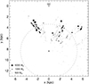 |
Fig. 1. Source distribution for the regions in our ALMAGAL sub-sample is shown as black dots. The size of the markers scales with the masses of the ALMAGAL clumps. Grey dots are the rest of the ALMAGAL survey and the dashed line is a heliocentric distance circle at 5 kpc. |
Observational parameters.
2.2. Sample
Looking at our sample, compared to the whole survey we check how the mass, luminosity, luminosity-to-mass ratio, and distance distributions compared to each other and whether there were signs of any bias. We see no signs of bias in distance, luminosity, or luminosity to mass ratio. For the mass we specifically chose regions over 500 M⊙ and, thus, this is reflected here. Histograms of these distributions can be found in Fig. A.1. For more information on how the survey parameters were calculated we refer to Molinari et al. (in prep.), but as an overview, the distances were derived with the Mège et al. (2021) method using the ALMAGAL spectral cubes and following this the distance dependent quantities were calculated.
2.3. Evolutionary stage
Before selecting the regions for the analysis, the ALMAGAL sample is classified by evolutionary sequence. We use the sequence and classification scheme defined by Urquhart et al. (2022), which divides the sources into four evolutionary stages: quiescent, protostellar, young stellar object (YSO), and HII regions. The classification is done by looking at the sources at three wavelengths: Hi-GAL 70 μm (Elia et al. 2017), MIPSGAL 24 μm (Carey et al. 2009), and GLIMPSE 8 μm (Churchwell et al. 2009). Quiescent sources have a central area free of emission at all three wavelengths. For protostellar sources, there is a point source in the 70 μm image, potentially a 24 μm counterpart, but the source is not visible in the 8 μm image. A YSO is detected as a point-like source at all three wavelengths. HII regions also have a point source at all three wavelengths but the source in the 8 μm image becomes more extended and ‘fluffy’.
Initially, the ALMAGAL sample was cross-matched with the ATLASGAL (Schuller et al. 2009; Urquhart et al. 2018, 2022) sample to see how many sources overlap and how many classifications can be immediately adopted. Cross-matching on Galactic coordinates with an error margin of 40″ leads to an initial match of roughly 600 regions out of 1013. The remaining ALMAGAL regions were classified visually according to the same rules as described above.
As an alternative evolutionary indicator, we can also look at the luminosity-to-mass ratio. This ratio increases with time, being very low in the early quiescent stage (e.g., Molinari et al. 2019; Elia et al. 2021). The distribution of the regions in each classification stage can be seen in Fig. 2a, where we have the peak luminosity-to-mass ratio progression as the cores become more evolved. Figure 2a enables a comparison of our evolutionary sequence with this evolutionary indicator and, as expected, the two classification schemes roughly agree, with some overlap. This can also be seen in Fig. 2b, showing a cumulative distribution. These classifications are done for the entire cluster-forming clump. However, within individual ALMAGAL regions, HII regions, YSO, protostellar, and even quiescent regions often coexist. Examples of this include NGC 6334I (e.g., Beuther et al. 2005) or G29.96+0.02 (e.g., Cesaroni et al. 1998, ISOSS J23053+5953 (Gieser et al. 2022).
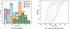 |
Fig. 2. Colour-coding for both figures is on evolutionary stage, legend shown in panel a. These plots show the sample of 17 quiescent, 23 protostellar, 22 YSO, and 25 HII regions. (a) Stacked histogram distribution of the luminosity-to-mass ratio for the regions in the ALMAGAL sub-sample being used for this work. (b) Individual cumulative distribution functions (CDF) of regions in each evolutionary stage, generated from kernel density estimates (KDEs) of the data shown in (a). |
2.4. Core identification
Each source in the subset of our ALMAGAL sample contains up to seven cores identified via the following process. We used the astrodendro1 programme on the continuum data for core identification, obtaining the peak position of these identified cores and estimating their peak and integrated flux density values. The astrodendro package allows us to break down the hierarchical structures in our observational data. The highest hierarchical level for each structure is a ‘leaf’ (i.e a structure with no substructure), these correspond to what we define as a core. We can see an example of a ‘leaf’ in Fig. 3, which shows the case of source AG348.5792–0.9197. The three main input parameters of astrodendro are min_value (the minimum pixel intensity to be considered), min_delta (the minimum height for any local maximum to be defined as an independent entity), and min_npix (the minimum number of pixels for a leaf to be defined as an independent entity). We decided to have a large significance level for the cores to be identified so that we were left dealing with just the cores themselves and their structures and not the extended parental cloud. We use min_value = 5σcont, min_delta = 5σcont and min_npix = beam area. With the combination of our choices of min_value and min_delta, all cores have a peak flux density ≥10σcont. Here, σcont or σline are the rms values of either the continuum image or the spectral cube for the lines being used. Running the analysis with these parameters, we were able to identify 203 cores within the 100 regions. Of these 100 regions, five regions had no cores identified with our criteria, so these were removed from the sample leaving an initial 95 regions with 203 cores. The official core catalogue for ALMAGAL calculated on the final data products, including also more extended ALMA configurations, will be available in Coletta et al. (in prep.).
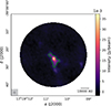 |
Fig. 3. Continuum image of ALMAGAL source AG348.5792–0.9197 from the astrodendro package where the green contours indicate the ‘leaves’ that are the areas we focus on here, namely: the cores. |
2.5. Analysis
We start the analysis with a detailed look into the main lines suitable for identifying outflows, such as SiO (5–4) and SO (65–54) and making position-velocity (PV) cuts along the filamentary structures surrounding each core (identified visually from the continuum contours, seen in Figs. 4 and 5a), in the H2CO (30, 3–20, 2) line.
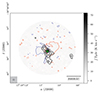 |
Fig. 4. Zeroth moment map of SO (65–54) in grey-scale for source AG348.5792–0.9197 overlaid with continuum contours in black (levels 3, 6, 9σcont). A green star to show the peak intensity position of the core. Red and blue contours show the ‘wings’ of the spectral line emission, from 3 to 20 km s−1 either side, with respect to the region velocity of rest. |
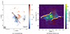 |
Fig. 5. Velocity analysis of source AG348.5792–0.9197. (a): First-moment map of YSO source AG348.5792–0.9197 in H2CO (30, 3–20, 2). The position of the continuum peak flux density is shown by the green star, and continuum contours are shown in black (levels 3, 6, 9σcont). The red line indicates the axis along which the PV cut was taken. (b): PV cut with 3 and 5σline contours in white, and the vlsr of the region shown by the white dashed line. The orange points show the nearest pixels at the 3σline contours. The red boxes are examples of the areas where we estimate the flow rates across (∼1″). The peak flux density position of the continuum core is located at the centre of each axis. |
2.5.1. Outflows
This work is primarily focussed on longitudinal flows along filamentary structures. To ensure there was no contamination from any associated outflows, we looked at the shock tracers available in the ALMAGAL survey. After a comparison of shock and outflow tracers SiO (5−4) and SO (65–54), it was evident that SO (65–54) presented the most outflow signatures, manifested as blue- and red-shifted line wing emission (‘wing’ structures on zeroth-moment maps, inspected visually, as seen in Fig. 4; also e.g., Widmann et al. 2016; van Gelder et al. 2021). It must be noted that these are not definite detections, just indications of outflows, and this decision was made by visually inspecting the data and results for both lines. We investigated the presence of any red and blue shifted SO (65–54) emission, before continuing with our analysis. Figure 4 shows an example of such an analysis, and we can see signatures of a bipolar outflow from the central core in source AG348.5792–0.9197 (denoted by a green star in the figure). We see red-shifted emission extending to the west and blue-shifted emission to the east, both almost perpendicular to the filamentary structure. With such an analysis, we can focus on the filamentary structures and calculate the flow rates along this axis without any major outflow contamination.
2.5.2. Position-velocity diagrams
Of all the strong lines available to use in the ALMAGAL spectral set-up, we decided to cut along the visibly elongated filamentary-like structures in the PV space using H2CO (30, 3–20, 2) due to its intermediate critical density (∼7 × 105 cm−3, Shirley 2015) that is similar to the densities we expect to trace in our regions. H2CO (30, 3–20, 2) is also a tracer of relatively cool gas (Eu/k 21 K) and can be used in combination with another H2CO line as a well-known temperature tracer (∼100 K e.g., Shirley 2015; Mangum & Wootten 1993; van der Tak et al. 2007; Gieser et al. 2021; Izumi et al. 2024). Abundance may vary by an order of magnitude over the evolutionary stages (Gerner et al. 2014).
The angle at which the PV cut was taken was determined by the outflow signatures and the filamentary structures. To ensure as little contamination from the potential outflows, the cut was made perpendicular to any signatures where possible, whilst keeping the cut inline with the filamentary structure. This is shown in Fig. 5. Any cores that did not have suitable emission in the PV cuts were removed from the sample (8 regions, 21 cores).
3. Flow rates
After sample selection, core identification, and line analysis the final sample consists of 87 regions with 182 cores in total. Table 2 shows how this sample is split among the evolutionary stages.
Final sample distribution.
3.1. Quantifying flow rates
To estimate the flow rates along the filamentary structures leading toward the cores, we follow the approach outlined in Beuther et al. (2020). The mass flows rates,  , are estimated as
 (1)
(1)
where Σ is the surface density in units of g cm−2 (converted from the column density calculated in Sect. 3.2), Δv is the velocity difference from the velocity of rest to the 3σline contour of the PV cut in km s−1, considered for the specific flow rate, and w is the width of the area along which the flow rate is measured in AU. The final values of  are converted to M⊙ yr−1. In the following, we describe the parameter determinations in more detail along with details of the calculation (see Appendix B).
3.2. Column density
Column density maps were made using Equation (2) (modified black body emission equation from Schuller et al. 2009) assuming optically thin dust emission at mm wavelengths (Hildebrand 1983) as follows:
 (2)
(2)
Here Fν is the continuum flux density, Bν(TD) is the Planck function for a dust temperature TD (see Sect. 3.3), Ω is the solid beam angle, μ is the mean molecular weight of the interstellar gas, assumed to be equal to 2.8, and mH is the mass of a hydrogen atom. We also assumed a gas-to-dust mass ratio of R = 150 (with the inclusion of heavy elements Draine 2011), along with κν = 0.899 cm2 g−1 (interpolated to 1300 μm from Table 1, col. 5 of Ossenkopf & Henning 1994). This was used to compute the column density for each pixel from the continuum image. The column density maps will be used to select the specific positions where we compute the mass flow rates. In addition to the column densities, we also estimated the core masses following Equation (3) below (e.g., as in Schuller et al. 2009):
 (3)
(3)
Here, we use the same values for κν and the gas-to-dust ratio, d, is the distance to the source, and Fν is taken from the integrated flux density from the cores (leaves) from the astrodendro analysis. Details of how we applied these values can be found in Sect. 4.4.
3.3. Temperature estimates
Different possibilities exist to estimate the temperatures needed for deriving the column density and mass. Individual estimates per core via molecular line emission of high-density tracers for the ALMAGAL sample will be presented in Jones et al. (in prep.). While we could use the dust temperatures derived from Hi-GAL (Molinari et al. 2010b), they have the disadvantage that they generally only sample the colder gas because of the Herschel far-infrared wavelength coverage and the large Herschel beam size. In a different approach, Molinari et al. (2016) and Traficante et al. (2023) calculated temperatures from spectral line emission, where they used luminosity to mass ratio (L/M) values as cut-off points for different temperatures. Following a similar approach, Coletta et al. (in prep.) have estimated temperatures that can be assigned to sources based on their evolutionary stage (indicated by luminosity to mass ratio):
Figure 6 shows the temperatures derived via these two approaches plotted against each other for each region. The gas temperatures show (as expected from Fig. 2b) that quiescent and protostellar sources have temperatures of 20 K, while at 35 K and above we see mostly YSOs and HII regions, with some exceptions. Comparing this with the dust temperatures where there are some YSO and HII region sources with dust temperature values below 15 K leads us to investigate further how this selection would affect the end result. The calculation of the flow rates was therefore done with both the Hi-GAL dust temperatures and the gas temperatures. Comparing the results there were no qualitative and only small quantitative differences (∼5−10%) so we are confident to proceed with the gas temperatures with the reasoning that the dust temperatures are tracing primarily cold gas, whereas the gas temperatures take the warmer protostellar cores into consideration, which is more aligned more with our aims.
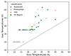 |
Fig. 6. Herschel derived dust temperature and the gas temperature plot against each other colour-coded in evolutionary stage. The grey dashed line shows the temperature equivalence line between the dust and the gas temperatures. |
3.4. Width
The width parameter, w, in Equation (1) is the width of the area along the filament we calculate the flow rate across. We took four areas along each PV cut to allow comparison between results at different offsets from the core. Two inner and two outer positions were chosen (0.75″ and 1.75″ away on either side of the core), excluding the central most 0.5″ (approximately half a beam size) to avoid contamination as this area is where the flows from all directions are merging. This width was taken as 1″, the approximate beam size of the data, for all four areas toward each core. An example of this is shown in Fig. 5b with the red box showing the width we are looking at to be 1″. With any conversion to linear distance, we have to take into account the range of distances to the sources in this work. Looking at our range of ∼2 to 6 kpc (see Fig. 1), the more distant sources could have linear width parameters up to a factor three higher. Given that our widths are defined by the (approximate) beam width, at larger distances we capture a larger physical scale and, hence, they are more likely to have diffuse gas within our source area. This, in turn, results in more distant sources typically having a lower average column density. While these distance effects may be possible, our derived flow rates show no significant distance dependence, hence, the effect should be small.
3.5. Velocity difference
To calculate a velocity difference we used the KeplerFit code from Bosco et al. (2019). The code works by dividing the PV cut into quadrants, taking the strongest (largest intensity) opposing quadrants and reading out the velocity values from the pixels that the specified σline contours go through (here we used 3σline). These points are highlighted in orange in Fig. 5b. The velocity measurements are then taken as the difference between the velocity value from the central pixel along the contour confined to each red box in Fig. 5b, and the velocity of rest (white dashed line in Fig. 5b). To use the region’s rest velocities as a proxy for the core velocities, we compared the rest velocity values to the velocities measured toward the core peak positions in the H2CO 1st moment maps. Comparing the difference between the two, we find that the majority of the values are less than our velocity resolution of 0.6 km s−1. In comparison to our median velocity difference measurement Δv of 3.4 km s−1, this is less than a 20% error margin. Considering that the ALMA H2CO emission is also affected by missing flux (see Sect. 3.6.1 for more information), especially near the peak velocities, this makes the rest velocity a good proxy for the reference velocity.
3.6. Error analysis
3.6.1. Data
Interferometric data without short spacing observations always suffer from missing flux. Regarding the continuum data, comparisons have been made to similar studies, for instance, the CORE project in the northern hemisphere, with 20 regions observed with a similar spectral set-up and similar baseline ranges. For instance, Beuther et al. (2018) estimated 60 to 90% missing flux across their range of sources in this context. Regarding the spectral line emission, typically the extended emission around the rest velocity is more strongly affected than compact emission offset from the rest velocity. Therefore the lower-level contours (outlined in Figure 5b) needed for the PV analysis are not strongly affected. Hence, we are confident that the velocity structure from the H2CO (30, 3–20, 2) line is relatively well recovered. Missing flux values impact our mass and column density estimates, so we took these values as lower limits.
3.6.2. Constants
For the gas-to-dust ratio, we used 150 (Draine 2011). The mean molecular weight of the ISM, μ, and the mass of a hydrogen atom, mH, both have standard values that were used in our equations (Draine 2003). The dust opacity, κν was chosen for our conditions and suitable wavelength. For different densities and ice mantels the value could vary up to 30–40%. Any uncertainties in these parameters here are considered minor compared to the systematic uncertainties discussed above and below. Overall, we are confident that the overall trends we observe will remain consistent.
3.6.3. Error propagation
We consider five of our parameters used across this project to have significant uncertainties. These are the flux density, temperature, distance, width, and velocity difference. To calculate the effects this has on our overall results we use Gaussian error propagation for each equation that contains one or more of these parameters. To calculate a mean, standardised error for each flow rate we use mean values combined with the following errors; for the flux density we take 10% from the calibration uncertainty, for temperature, we take 5 K, for the distance we assume a kinematic distance error of 0.5 kpc, for width we take 0.1″ for on sky offset discrepancy and finally for the velocity differences we take the spectral resolution of 0.6 km s−1 as the error from the nearest pixel approximation. When combining these we end up with ±50% error margins on our final flow rates. For the core mass, we also estimate roughly ±50% error margins using flux density, temperature, and distance in the Gaussian error propagation.
3.6.4. Inclination angle
We set the inclination angle, i, to 0 for the filamentary structures in the plane of the sky. Our input parameters are all affected by the unknown inclination angles. Considering these, Equation 1 becomes Equation (4), below (full derivation can be found in Appendix A).
 (4)
(4)
Here, we are left with a correction factor of  . Hence, the inclination clearly affects the results, meaning our flow rate results have a more narrow distribution in reality as tan(i) will both increase and decrease with the inclination angle. In order to check for the potential spreading of the observed flow rates due to the unknown inclination angle between the filament direction and the observer’s line-of-sight, we compute analytically the spreading for an idealised case: We assume a sample of an arbitrary number of filaments with an universal flow rate of
  M⊙ yr−1 along all filamentary structures of the sample. We approximate the filaments as cylindrical tube-like structures with a constant and uniform flow rate, hereafter called the ‘real’ flow rate,
  . The corresponding probability density of the observed flow rates is then given as
 (5)
(5)
We binned the flow rates in the range from 10−6 M⊙ yr−1 to 10−2 M⊙ yr−1 into 60 bins with uniform binning width in log space and compute the observational probability by numerically integrating the probability density over the bin. The final outcome is presented in Fig. 7.
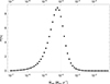 |
Fig. 7. Theoretical spreading of the observed flow rate due to unknown inclination of the filament for a tube-like cylindrical filament model with a universal flow rate of |

The peak of the probability distribution is quite close to the true flow rate, especially compared to the overall uncertainties of the measurement of the observed flow rates. Also the spread is acceptable with a full width at half maximum (FWHM) of the distribution of quite exactly one order of magnitude in observed flow rate.
In reality, the longer slope toward smaller flow rates will be further reduced (i.e. it will attain a lower probability to be observed) due to the fact that in the simple tube-like model the flow velocity is always aligned with the filament axis and an observer at an inclination of i = 0 is assumed to measure zero velocity; in reality, there will be a non-zero velocity in those directions, which, in turn, reduces the likelihood for observations of the smallest flow rates. Furthermore, a real sample of filaments will most likely deviate from the assumption of an universal flow rate through all filaments. This will yield an additional spreading of the distribution of observed flow rates, which is purposely not taken into account in our analytical model; our analysis is focussed on the effect of the unknown inclinations only.
4. Results
Following the initial analysis and methodology laid out in Sections 2.5 and 3 we present the results for our sample, which using the parameters discussed in Sect. 3 contains 728 measured flow rates. These are mainly constrained between 10−6 M⊙ yr−1 and 10−2 M⊙ yr−1, with the average values being on the order of 10−4 M⊙ yr−1, which is conducive to forming a high-mass star in a few hundred thousand years (e.g., McKee & Tan 2003; Beuther et al. 2007; Zinnecker & Yorke 2007; Tan et al. 2014; Motte et al. 2018). All flow rates can be found in Table D.2.
Our general assumption for the estimated flow rates is that they are directional toward the cores and hence they are accretion flows. This should certainly be valid for the earlier evolutionary stages: quiescent, protostellar, and YSO. However, that is less clear for the HII regions. If we have evolving HII regions, those could already be pushing the gas outwards. Hence, the HII flow rates are not necessarily accretion flows. An individual classification of each core is beyond the scope of this paper.
4.1. Statistical testing
To determine the statistical relevance of the results we applied two different, well-known, significance tests, the Kolmogorov–Smirnov (KS) test and the Mann-Whitney U test (Chakravarti et al. 1967; McKnight & Najab 2010). Both tests are non-parametric, making them suitable for data that may not follow a normal distribution. The KS test is focussed on the entire distribution function, while the Mann-Whitney U test looks at the ranks of observations. Both tests generate probability values (p-values) and the interpretation is based on comparing the p-value to a chosen significance level. Here, we use 0.05, as used by Chakravarti et al. (1967). The null hypothesis for both tests is the assumption that the samples come from the same distribution (KS) or population (Mann-Whitney U). The KS test generates a p-value, indicating the probability of observing the observed or more extreme differences if the samples come from the same distribution. The Mann-Whitney U test generates a p-value, indicating the probability of observing the calculated U statistic or a more extreme value if the samples come from the same population.
If our p values from either test are greater than 0.05 then any difference between the distributions is sufficiently small as to be not significant. These results are discussed in Sections 4.2, 4.3, and 4.4 below.
4.2. Evolutionary stage
Looking at our flow rates in the context of evolutionary stage may tell us about how the accretion process changes as a (proto)star evolves. This result is presented in Figure 8. The four panels show the distribution for each evolutionary stage from quiescent to the HII regions. Considering the ±50% errors, there is a trend between the means and medians of these sub-samples, most notably between Protostellar and YSO sources. In terms of outliers, we have a few that can be seen in Figure 8. Outliers on the lower end are present in the earlier stages: quiescent and protostellar, and on the higher end in the more evolved sources. KS and Mann-Whitney tests were done for each combination of the four data sets, the p-value results can be seen in Table 3. Using a significance level of 5%, any p-value above 0.05 tells us there is likely no statistical difference between the data sets. We see that quiescent sources in combination with any of the others are likely not from the same distribution using the KS test however the Mann-Whitney p-value suggests these are not statistically different. By eye, we see there is an increasing trend in the mean or median flow rate through the evolutionary stages. We also note the similarity between these histograms and the distribution in Fig. 7, looking at the theoretical spreading due to unknown inclination angle. This gives us an idea that the spread we see in these results is likely partly due to the unknown inclination angle for our observational data.
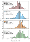 |
Fig. 8. Histograms of the flow rate results for cores in each evolutionary stage quiescent to HII region from top to bottom. The mean and median are shown by the black dashed and grey solid lines, respectively, in each panel. |
p-values from the KS and Mann-Whitney U tests.
4.3. Offset from the core
We now discuss whether the flow rate changes with offset from the core. We look specifically at sections that are 1″ in width at offsets from the central coordinates of 0.75 and 1.75″ away on either side of the core, along the filamentary axis. Figure 9 shows the distributions for the flow rates at 0.75″ (inner) and 1.75″ (outer) offsets. We see these two distributions have very similar median values but their means are qualitatively different by approximately a factor of two. Again, to determine if these two data sets have a significant difference KS and Mann-Whitney tests were performed (more information in Sect. 4.1). The p-values from the two tests were 0.0691 and 0.0731 respectively. Using our significance level of 0.05, we cannot reject the null hypothesis that these two distributions are from the same origin. As a further analysis, we looked at the difference between the inner and outer flow rates per core. The distribution can be seen in Fig. 10 where we can see the distribution centered around 0, with less than 0 meaning the core had higher flow rates further away along the filamentary structure and more than 0 meaning the core has higher flow rates closer to the centre of the core. With a median of 1.12 × 10⁻⁵ M⊙ yr−1, we see a trend that the inner flow rates are larger than the outer ones.
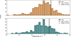 |
Fig. 9. Histograms of the flow rate results in the context of offset from the core. The top panel shows the results from the inner regions and the bottom from those further from the core. |
4.4. Core mass
Taking the integrated flux values for each core from the identification analysis (see Sect. 2.5) we calculated individual core masses, using Equation (3). The distribution of the flow rates vs. core mass is shown in Fig. 11 and we see a clear trend between the mass of these cores and the rate at which the material flows onto them. Overlaid in Fig. 11 in grey are the same points now binned, first per core (as there are four values per core), and then along the sample. Here we also have a line of best fit through these binned values. This suggests that we have a relationship where the flow rate follows ∼M2/3. We also looked to see if there was a relationship between these flow rates and the mass of the parental clump and we found no correlation. This indicates that flow rates are largely independent from the parental gas clump and that the found correlation is constrained to the smaller core scales.
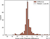 |
Fig. 10. A histogram showing the distribution of the difference between the inner and outer flow rates per core ( |

As mentioned in Sect. 2.2 we looked into whether the sample had any bias’ with respect to the whole ALMAGAL sample. Here we want to see if the distance spread, offset or evolutionary stage is causing any unexpected effects. We find no correlation between these flow rates and the distances of these clumps. For the offsets, the distance from the cores, we find that only taking into account the two flow rates closer to the cores gives a steeper relation than the one presented in Fig. 11 and if we look at just the flow rates further away from the cores we get a flatter relation. This is not surprising and is in support of Fig. 10 where we show that the inner flow rates are systematically larger than the outer ones. Comparative higher flow rates closer to the centre and a steeper relation with core mass are supportive that indeed gravity is dominating the infall dynamics. Figures with these relations shown can be found in Appendix C.
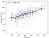 |
Fig. 11. Scatter plot of the results of the whole sample showing flow rate vs. core mass in grey. The purple points are the average flow rate/mass values per bin, with the associated errors. Here, each bin contains the same number of cores. A line of best fit is shown in black. |
This is not the first time that a correlation between core mass and accretion rate has been found and or discussed in the literature. Beltrán & de Wit (2016) compiled YSOs with a range of masses and looked at the relationship between their mass and their accretion rates, getting an overall relationship proportional to ∼M2. During our analysis this relationship was looked at per evolutionary stage to see if (in Fig. 11) we were seeing any of the evolutionary stages clumped together; however, we found this was not the case. We cannot comment on a specific relationship for our YSO values. Clark & Whitworth (2021) discuss what the resulting exponent in this relationship can mean in terms of different mass accretion mechanisms and also the star clusters system mass function. The two accretion mechanisms they discuss are tidal-lobe and Bondi-Hoyle (Bonnell et al. 2001). It is thought that tidal-lobe dominates when the potential of the cluster is still dominated by gas, this mechanism has an exponent of 2/3. The Bondi-Hoyle accretion mechanism dominates when the potential in the cluster is dominated by proto-systems, this mechanism has exponent 2. Our results are in clear agreement with the tidal-lobe accretion mechanism where the potential is dominated by the gas. This is consistent with the ALMAGAL sample covering early evolutionary stages.
5. Discussion
5.1. Comparison between low- and high-mass regions
In this section, we discuss how the flow rates estimated in this work compare to previous studies that quantitatively describe flow rates. The flow rates we present here are comparable to others in the literature for different mass ranges and scales (e.g., López-Sepulcre et al. 2010; Duarte-Cabral et al. 2013; Kirk et al. 2013; Peretto et al. 2013; Henshaw et al. 2014; Traficante et al. 2017; Beuther et al. 2020; Sanhueza et al. 2021; Redaelli et al. 2022). Looking at an example from the low mass case, Kirk et al. (2013) uses their Mopra survey of multiple molecular emission lines to look for possible accretion flows onto the central cluster. They present values on the order of 2.8 × 10⁻⁵ M⊙ yr−1. For an example of a high mass region, Henshaw et al. (2014) investigates the filamentary structure of an infrared dark cloud G035.39−00.33 in N2H+ and finds mass accretion rates of 7 × 10⁻⁵ M⊙ yr−1 with individual filaments feeding individual cores. An example with varying distances from the core is shown in Beuther et al. (2020). The authors looked at infrared dark cloud G28.3 using 13CO and, depending on the distance from the core, they presented values around 5 × 10⁻⁵ M⊙ yr−1. If we zoom out and look at larger clumps, we see that Traficante et al. (2017) reported mass accretion rates between 0.04 × 10⁻³ and 2 × 10⁻³ M⊙ yr−1. They also reported seeing an apparent increase in the accretion rate depending on the presence of embedded 24 μm sources. This correlates to seeing a difference between our less evolved protostellar sources and more evolved YSO sources.
The results presented here are consistent with the results from the works in the literature mentioned above. The work done by Kirk et al. (2013) in the Serpens South region results are between a factor of 10 and 1000 times smaller than the results we present. If we think about the relationship between flow rate and core mass shown in Sect. 4.4 this is to be expected. Furthermore, comparing low to high-mass star formation, actual accretion rates in the high-mass regime tend to be much higher. There are many competing models discussing the formation timescale of high mass stars (e.g., Bonnell et al. 1998, 2001, 2007; McKee & Tan 2003; Beuther et al. 2007; Hartmann et al. 2012; Tan et al. 2014; Motte et al. 2018) giving approximately 105–106 years. This then explains that our protostellar and YSO sources, similar to the one studied in Henshaw et al. (2014), exhibit very similar results.
5.2. Comparison to simulations
Observational studies and theoretical models are extremely complementary to each other for advancing our knowledge in many topics. Here we compare our results to theoretical models that have quantitatively produced accretion flow rates, looking specifically at the work done by Padoan et al. (2020) and Gómez & Vázquez-Semadeni (2014).
Looking at the simulations by Padoan et al. (2020), they produce a sample of roughly 1500 stars within a volume of 250 pc and study the physical conditions surrounding the sample. The range of this simulation provides a large statistical sample of massive stars, forming realistic distributions of initial conditions. They present mean mass accretion rates on the order of ∼10−5 M⊙ yr−1 onto the core and they also look at the mass accretion rate 1 pc away from the core and find it increases by an order of magnitude, which agrees with Traficante et al. (2017) on their values for larger scale accretion rates. They also state that their largest values are nearly ten times higher than these mean values. The range of results we get from our sample agrees with the orders of magnitude discussed in their work. They go on to discuss whether the accretion rate grows systematically with time. We agree with their interpretation that this is not systematic (in their case, at the ends of the prestellar phase; whereas in our case, it is throughout our evolutionary sequence).
Turning to Gómez & Vázquez-Semadeni (2014), they simulate the formation of a molecular cloud from converging gas flows resulting in a dynamic cloud with a lot of substructures, and the cloud grows due to accretion through filamentary structures channelling gas onto the clumps. They look at accretion rates radially along the filament and see a dependence that correlates to changes in the column density profile along the filament. Whilst the method produces filamentary structures the difference in scale makes it hard for a complete interpretation and comparison. Taking into account our work and the examples in this discussion, there are definite similarities. The discussion of perpendicular versus parallel flows looking at accretion onto the filament itself and then along towards the central clump is also something discussed by many of these works. In the study by Gómez & Vázquez-Semadeni (2014), they looked at flows both along the filament and perpendicular and even compared themselves to the perpendicular results in Kirk et al. (2013), along with similar values; however, they also pointed out that their scales are slightly different.
6. Conclusions
This work aims to answer the question: what the properties are of accretion flows in high-mass star-forming clusters. This paper presents a subset of the regions from the ALMAGAL survey chosen to investigate the properties of flow rates, focussing specifically on longitudinal flows along filamentary structures towards the central core. A summary of our main results is as follows:
-
Using calculated column density values and derived velocity differences based on H2CO (30, 3–20, 2) emission, we were able to estimate flow rates for 182 cores from 87 regions of the ALMAGAL survey. We got flow rates on average on the order of ∼10−4 M⊙ yr−1 with error margins of ±50%.
-
We see trends of increasing flow rates through the evolutionary stages and along the filamentary structure, increasing as we get closer to the central cores.
-
We also see a relationship between the flow rates and the masses of these cores of ∼M2/3, which supports the tidal-lobe accretion mechanism.
-
Our results are in line with other observational studies and complementary to theoretical studies in the literature using different methods and mass ranges. Specifically, from the examples discussed, our flow rates are consistent with Padoan et al. (2020); however, we were not able to directly make any comparison to Gómez & Vázquez-Semadeni (2014).
In addition to the conclusions drawn from this project, it is worth noting several supplementary contributions. This includes evolutionary classifications that have been assigned to the whole ALMAGAL sample to allow for analysis in the context of evolutionary stage and outflow signatures being detected in this ALMAGAL sub-sample using the SO (65–54) spectral line; this is done by looking at the ‘wings’ of the spectra. Building on the trends we have seen in this work, some important next steps would be to see what these relationships look like at both smaller and larger scales and how these are linked to each other.
Data availability
Tables D.1 and D.2 are available at the CDS via anonymous ftp to cdsarc.cds.unistra.fr (130.79.128.5) or via https://cdsarc.cds.unistra.fr/viz-bin/cat/J/A+A/690/A185
Acknowledgments
The authors thank Felix Bosco and Daniel Seifried for their discussions during this work and the use of the KeplarFit code by FB. We would also like to thank the referee for the insightful comments and suggestions that improved the paper during the submission process. This research made significant use of astrodendro, a Python package to compute dendrograms of Astronomical data (http://www.dendrograms.org/), Astropy (http://www.astropy.org): a community-developed core Python package and an ecosystem of tools and resources for astronomy (Astropy Collaboration 2013, 2018, 2022), NumPy (Harris et al. 2020), matplotlib (Hunter 2007) and Spectral-Cube (Ginsburg et al. 2019). This paper makes use of the following ALMA data: ADS/JAO.ALMA2019.1.00195.L. ALMA is a partnership of ESO (representing its member states), NSF (USA), and NINS (Japan), together with NRC (Canada), MOST and ASIAA (Taiwan), and KASI (Republic of Korea), in cooperation with the Republic of Chile. The Joint ALMA Observatory is operated by ESO, AUI/NRAO and NAOJ. RSK acknowledges financial support from the European Research Council via the ERC Synergy Grant “ECOGAL” (project ID 855130), from the German Excellence Strategy via the Heidelberg Cluster of Excellence (EXC 2181 – 390900948) “STRUCTURES”, and from the German Ministry for Economic Affairs and Climate Action in project “MAINN” (funding ID 50OO2206). RSK also thanks for computing resources provided by the Ministry of Science, Research and the Arts (MWK) of the State of Baden-Württemberg through bwHPC and the German Science Foundation (DFG) through grants INST 35/1134-1 FUGG and 35/1597-1 FUGG, and also for data storage at SDS@hd funded through grants INST 35/1314-1 FUGG and INST 35/1503-1 FUGG. Part of this research was carried out at the Jet Propulsion Laboratory, California Institute of Technology, under a contract with the National Aeronautics and Space Administration (80NM0018D0004). RK acknowledges financial support via the Heisenberg Research Grant funded by the Deutsche Forschungsgemeinschaft (DFG, German Research Foundation) under grant no. KU 2849/9, project no. 445783058. T.L. acknowledges support from the National Key R&D Program of China (No. 2022YFA1603100); the National Natural Science Foundation of China (NSFC), through grants No. 12073061 and No. 12122307; the international partnership programme of the Chinese Academy of Sciences, through grant No. 114231KYSB20200009; and the Shanghai Pujiang Program 20PJ1415500. SW gratefully acknowledges funding via the Collaborative Research Center 1601 (sub-project A5) funded by the German Science Foundation (DFG). A.S.-M. acknowledges support from the RyC2021-032892-I grant funded by MCIN/AEI/10.13039/501100011033 and by the European Union ‘Next GenerationEU’/PRTR, as well as the programme Unidad de Excelencia María de Maeztu CEX2020-001058-M, and support from the PID2020-117710GB-I00 (MCI-AEI-FEDER, UE). PS was partially supported by a Grant-in-Aid for Scientific Research (KAKENHI Number JP22H01271 and JP23H01221) of JSPS. GAF gratefully acknowledges funding via the Collaborative Research Center 1601 (sub-project A2) funded by the German Science Foundation (DFG) and from the University of Cologne through its Global Faculty Program.
References
- Alves, J., Zucker, C., & Goodman, A. 2020, Nature, 578, 237 [NASA ADS] [CrossRef] [Google Scholar]
- André, P., Men’shchikov, A., Bontemps, S., et al. 2010, A&A, 518, L102 [NASA ADS] [CrossRef] [EDP Sciences] [Google Scholar]
- Arce, H. G., Shepherd, D., Gueth, F., et al. 2007, in Protostars and Planets V, eds. B. Reipurth, D. Jewitt, & K. Keil, 245 [Google Scholar]
- Astropy Collaboration (Robitaille, T. P., et al.) 2013, A&A, 558, A33 [NASA ADS] [CrossRef] [EDP Sciences] [Google Scholar]
- Astropy Collaboration (Price-Whelan, A. M., et al.) 2018, AJ, 156, 123 [Google Scholar]
- Astropy Collaboration (Price-Whelan, A. M., et al.) 2022, ApJ, 935, 167 [NASA ADS] [CrossRef] [Google Scholar]
- Beltrán, M. T., & de Wit, W. J. 2016, A&ARv, 24, 6 [Google Scholar]
- Beuther, H., Thorwirth, S., Zhang, Q., et al. 2005, ApJ, 627, 834 [CrossRef] [Google Scholar]
- Beuther, H., Zhang, Q., Bergin, E. A., et al. 2007, A&A, 468, 1045 [NASA ADS] [CrossRef] [EDP Sciences] [Google Scholar]
- Beuther, H., Mottram, J. C., Ahmadi, A., et al. 2018, A&A, 617, A100 [NASA ADS] [CrossRef] [EDP Sciences] [Google Scholar]
- Beuther, H., Wang, Y., Soler, J., et al. 2020, A&A, 638, A44 [NASA ADS] [CrossRef] [EDP Sciences] [Google Scholar]
- Bonnell, I. A., Bate, M. R., & Zinnecker, H. 1998, MNRAS, 298, 93 [Google Scholar]
- Bonnell, I. A., Clarke, C. J., Bate, M. R., & Pringle, J. E. 2001, MNRAS, 324, 573 [NASA ADS] [CrossRef] [Google Scholar]
- Bonnell, I. A., Bate, M. R., & Vine, S. G. 2003, MNRAS, 343, 413 [NASA ADS] [CrossRef] [Google Scholar]
- Bonnell, I. A., Larson, R. B., & Zinnecker, H. 2007, in Protostars and Planets V, eds. B. Reipurth, D. Jewitt, & K. Keil, 149 [Google Scholar]
- Bosco, F., Beuther, H., Ahmadi, A., et al. 2019, A&A, 629, A10 [NASA ADS] [CrossRef] [EDP Sciences] [Google Scholar]
- Bressert, E., Bastian, N., Gutermuth, R., et al. 2010, MNRAS, 409, L54 [NASA ADS] [Google Scholar]
- Carey, S. J., Noriega-Crespo, A., Mizuno, D. R., et al. 2009, PASP, 121, 76 [Google Scholar]
- Cesaroni, R., Hofner, P., Walmsley, C. M., & Churchwell, E. 1998, A&A, 331, 709 [Google Scholar]
- Chakravarti, I. M., Laha, R. G., & Roy, J. 1967, Handbook of Methods of Applied Statistics (New York: John Wiley and Sons) [Google Scholar]
- Churchwell, E., Babler, B. L., Meade, M. R., et al. 2009, PASP, 121, 213 [Google Scholar]
- Clark, P. C., & Whitworth, A. P. 2021, MNRAS, 500, 1697 [Google Scholar]
- Draine, B. T. 2003, ApJ, 598, 1017 [NASA ADS] [CrossRef] [Google Scholar]
- Draine, B. T. 2011, Physics of the Interstellar and Intergalactic Medium (Princeton: Princeton University Press) [Google Scholar]
- Duarte-Cabral, A., Bontemps, S., Motte, F., et al. 2013, A&A, 558, A125 [NASA ADS] [CrossRef] [EDP Sciences] [Google Scholar]
- Elia, D., Molinari, S., Schisano, E., et al. 2017, MNRAS, 471, 100 [NASA ADS] [CrossRef] [Google Scholar]
- Elia, D., Merello, M., Molinari, S., et al. 2021, MNRAS, 504, 2742 [NASA ADS] [CrossRef] [Google Scholar]
- Frank, A., Ray, T. P., Cabrit, S., et al. 2014, in Protostars and Planets VI, eds. H. Beuther, R. S. Klessen, C. P. Dullemond, & T. Henning, 451 [Google Scholar]
- Gerner, T., Beuther, H., Semenov, D., et al. 2014, A&A, 563, A97 [NASA ADS] [CrossRef] [EDP Sciences] [Google Scholar]
- Gieser, C., Beuther, H., Semenov, D., et al. 2021, A&A, 648, A66 [EDP Sciences] [Google Scholar]
- Gieser, C., Beuther, H., Semenov, D., et al. 2022, A&A, 657, A3 [CrossRef] [EDP Sciences] [Google Scholar]
- Ginsburg, A., Koch, E., Robitaille, T., et al. 2019, https://doi.org/10.5281/zenodo.2573901 [Google Scholar]
- Goldsmith, P. F., Heyer, M., Narayanan, G., et al. 2008, ApJ, 680, 428 [Google Scholar]
- Gómez, G. C., & Vázquez-Semadeni, E. 2014, ApJ, 791, 124 [Google Scholar]
- Hacar, A., Clark, S. E., Heitsch, F., et al. 2023, ASP Conf. Ser., 534, 153 [NASA ADS] [Google Scholar]
- Harris, C. R., Millman, K. J., van der Walt, S. J., et al. 2020, Nature, 585, 357 [NASA ADS] [CrossRef] [Google Scholar]
- Hartmann, L., Ballesteros-Paredes, J., & Heitsch, F. 2012, MNRAS, 420, 1457 [Google Scholar]
- Henshaw, J. D., Caselli, P., Fontani, F., Jiménez-Serra, I., & Tan, J. C. 2014, MNRAS, 440, 2860 [Google Scholar]
- Hildebrand, R. H. 1983, QJRAS, 24, 267 [NASA ADS] [Google Scholar]
- Hoare, M. G., Lumsden, S. L., Oudmaijer, R. D., et al. 2005, in Massive Star Birth: A Crossroads of Astrophysics, eds. R. Cesaroni, M. Felli, E. Churchwell, & M. Walmsley, 227, 370 [NASA ADS] [Google Scholar]
- Hunter, J. D. 2007, Comput. Sci. Eng., 9, 90 [NASA ADS] [CrossRef] [Google Scholar]
- Izumi, N., Sanhueza, P., Koch, P. M., et al. 2024, ApJ, 963, 163 [NASA ADS] [CrossRef] [Google Scholar]
- Jackson, J. M., Finn, S. C., Chambers, E. T., Rathborne, J. M., & Simon, R. 2010, ApJ, 719, L185 [Google Scholar]
- Kahn, F. D. 1974, A&A, 37, 149 [NASA ADS] [Google Scholar]
- Kirk, H., Myers, P. C., Bourke, T. L., et al. 2013, ApJ, 766, 115 [Google Scholar]
- Kuiper, R., & Hosokawa, T. 2018, A&A, 616, A101 [NASA ADS] [CrossRef] [EDP Sciences] [Google Scholar]
- Lada, C. J., & Lada, E. A. 2003, ARA&A, 41, 57 [Google Scholar]
- López-Sepulcre, A., Cesaroni, R., & Walmsley, C. M. 2010, A&A, 517, A66 [NASA ADS] [CrossRef] [EDP Sciences] [Google Scholar]
- Lumsden, S. L., Hoare, M. G., Urquhart, J. S., et al. 2013, ApJS, 208, 11 [Google Scholar]
- Mangum, J. G., & Wootten, A. 1993, ApJS, 89, 123 [Google Scholar]
- McKee, C. F., & Tan, J. C. 2003, ApJ, 585, 850 [Google Scholar]
- McKnight, P. E., & Najab, J. 2010, The Corsini Encyclopedia of Psychology, 1 [Google Scholar]
- Mège, P., Russeil, D., Zavagno, A., et al. 2021, A&A, 646, A74 [NASA ADS] [CrossRef] [EDP Sciences] [Google Scholar]
- Molinari, S., Swinyard, B., Bally, J., et al. 2010a, A&A, 518, L100 [NASA ADS] [CrossRef] [EDP Sciences] [Google Scholar]
- Molinari, S., Swinyard, B., Bally, J., et al. 2010b, PASP, 122, 314 [Google Scholar]
- Molinari, S., Merello, M., Elia, D., et al. 2016, ApJ, 826, L8 [Google Scholar]
- Molinari, S., Baldeschi, A., Robitaille, T. P., et al. 2019, MNRAS, 486, 4508 [Google Scholar]
- Motte, F., Bontemps, S., & Louvet, F. 2018, ARA&A, 56, 41 [NASA ADS] [CrossRef] [Google Scholar]
- Myers, P. C. 2009, ApJ, 700, 1609 [Google Scholar]
- Offner, S. S. R., Clark, P. C., Hennebelle, P., et al. 2014, in Protostars and Planets VI, eds. H. Beuther, R. S. Klessen, C. P. Dullemond, & T. Henning, 53 [Google Scholar]
- Olguin, F. A., Sanhueza, P., Chen, H.-R. V., et al. 2023, ApJ, 959, L31 [NASA ADS] [CrossRef] [Google Scholar]
- Ossenkopf, V., & Henning, T. 1994, A&A, 291, 943 [NASA ADS] [Google Scholar]
- Padoan, P., Pan, L., Juvela, M., Haugbølle, T., & Nordlund, Å. 2020, ApJ, 900, 82 [NASA ADS] [CrossRef] [Google Scholar]
- Peretto, N., Fuller, G. A., Duarte-Cabral, A., et al. 2013, A&A, 555, A112 [NASA ADS] [CrossRef] [EDP Sciences] [Google Scholar]
- Redaelli, E., Bovino, S., Sanhueza, P., et al. 2022, ApJ, 936, 169 [NASA ADS] [CrossRef] [Google Scholar]
- Salpeter, E. E. 1955, ApJ, 121, 161 [Google Scholar]
- Sanhueza, P., Girart, J. M., Padovani, M., et al. 2021, ApJ, 915, L10 [NASA ADS] [CrossRef] [Google Scholar]
- Scalo, J. M. 1985, in Protostars and Planets II, eds. D. C. Black, & M. S. Matthews, 201 [Google Scholar]
- Schisano, E., Molinari, S., Elia, D., et al. 2020, MNRAS, 492, 5420 [Google Scholar]
- Schneider, N., Csengeri, T., Bontemps, S., et al. 2010, A&A, 520, A49 [CrossRef] [EDP Sciences] [Google Scholar]
- Schuller, F., Menten, K. M., Contreras, Y., et al. 2009, A&A, 504, 415 [NASA ADS] [CrossRef] [EDP Sciences] [Google Scholar]
- Shirley, Y. L. 2015, PASP, 127, 299 [Google Scholar]
- Smith, R. J., Longmore, S., & Bonnell, I. 2009, MNRAS, 400, 1775 [Google Scholar]
- Svoboda, B. E., Shirley, Y. L., Traficante, A., et al. 2019, ApJ, 886, 36 [Google Scholar]
- Syed, J., Soler, J. D., Beuther, H., et al. 2022, A&A, 657, A1 [NASA ADS] [CrossRef] [EDP Sciences] [Google Scholar]
- Tackenberg, J., Beuther, H., Henning, T., et al. 2014, A&A, 565, A101 [NASA ADS] [CrossRef] [EDP Sciences] [Google Scholar]
- Tan, J. C., Beltrán, M. T., Caselli, P., et al. 2014, Protostars and Planets VI (Tucson: University of Arizona Press) [Google Scholar]
- Thomasson, B., Joncour, I., Moraux, E., et al. 2022, A&A, 665, A119 [NASA ADS] [CrossRef] [EDP Sciences] [Google Scholar]
- Traficante, A., Fuller, G. A., Billot, N., et al. 2017, MNRAS, 470, 3882 [Google Scholar]
- Traficante, A., Jones, B. M., Avison, A., et al. 2023, MNRAS, 520, 2306 [NASA ADS] [CrossRef] [Google Scholar]
- Urquhart, J. S., Busfield, A. L., Hoare, M. G., et al. 2007, A&A, 474, 891 [NASA ADS] [CrossRef] [EDP Sciences] [Google Scholar]
- Urquhart, J. S., König, C., Giannetti, A., et al. 2018, MNRAS, 473, 1059 [Google Scholar]
- Urquhart, J. S., Wells, M. R. A., Pillai, T., et al. 2022, MNRAS, 510, 3389 [NASA ADS] [CrossRef] [Google Scholar]
- van der Tak, F. F. S., Black, J. H., Schöier, F. L., Jansen, D. J., & van Dishoeck, E. F. 2007, A&A, 468, 627 [NASA ADS] [CrossRef] [EDP Sciences] [Google Scholar]
- van Gelder, M. L., Tabone, B., van Dishoeck, E. F., & Godard, B. 2021, A&A, 653, A159 [CrossRef] [EDP Sciences] [Google Scholar]
- Widmann, F., Beuther, H., Schilke, P., & Stanke, T. 2016, A&A, 589, A29 [NASA ADS] [CrossRef] [EDP Sciences] [Google Scholar]
- Williams, J. P., Blitz, L., & McKee, C. F. 2000, in Protostars and Planets IV, eds. V. Mannings, A. P. Boss, & S. S. Russell, 97 [Google Scholar]
- Wolfire, M. G., & Cassinelli, J. P. 1987, ApJ, 319, 850 [NASA ADS] [CrossRef] [Google Scholar]
- Yorke, H. W., & Kruegel, E. 1977, A&A, 54, 183 [NASA ADS] [Google Scholar]
- Zhang, Q., Wang, K., Lu, X., & Jiménez-Serra, I. 2015, ApJ, 804, 141 [Google Scholar]
- Zinnecker, H. 1984, MNRAS, 210, 43 [Google Scholar]
- Zinnecker, H., & Yorke, H. W. 2007, ARA&A, 45, 481 [Google Scholar]
Appendix A: Sample parameter Hhstograms
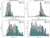 |
Fig. A.1. Histograms comparing the all regions in the ALMAGAL survey versus those ones chosen for this sample for distance, mass, luminosity, and L/M. |
Appendix B: Derivation of flow rate along a filament
In this appendix, we present a derivation of the formula used for the observational measurement of the flow rates along filamentary structures. We start from mass conservation in hydrodynamics, namely the continuity equation:
 (B.1)
(B.1)
with the density as ρ and the velocity as v. If we represent the filament as a cylindrical object and we check for the temporal change of mass within a section of the cylinder of real length, wr, and fixed volume, V, we can take the volume out of the time derivative as:
 (B.2)
(B.2)
If we further approximate the medium density to be uniform along the spatial scale of interest wr, we take the density out of the spatial derivative, and the volume, V, cancels out:
 (B.3)
(B.3)
For a one-dimensional (1D) flow along the filament, we can approximate the divergence of the velocity field, ∇ ⋅ v, as the velocity difference Δvout − in of the flow out of the section of length, wr, and into it:
 (B.4)
(B.4)
Equation (B.4) represents the mass conservation within the section wr of the filament. As an example: For a uniform velocity field, the inflow and outflow velocities are identical Δvout − in = 0 and the mass within the section remains unchanged.
To obtain a formula for the flow rate  , we have to substitute the velocity difference by the absolute, local velocity vr of the flow (subscript "r" meaning the real values and subscript "obs" the corresponding observed values):
 (B.5)
(B.5)
Here, we included the convention that the flow rate is always treated as a positive value, regardless if the flow is pointing towards the observer or away from the observer.
So far, we have discussed the system only in its local (unobserved) properties. Now let’s introduce the observational properties: The absolute, local velocity vr can be obtained from the observational data by subtracting the systemic velocity vsys from the observed velocity vobs with Δvr = |vobs − vsys|:
 (B.6)
(B.6)
The mass MV can be approximated by the column density Σ times the beam. Since we use 1″ length scale, roughly a beam width, we can approximate the beam with
 (B.7)
(B.7)
Substituting in the beam area, we get
 (B.8)
(B.8)
where we chose our measured length scale as the size of the beam. Including now the inclination dependence of the observed parameters:
 (B.9)
(B.9)
and
 (B.10)
Substituting Equations (B.8)-(B.10) into Equation (B.6) we get
 (B.11)
which in its final form is
 (B.12)
Appendix C: Core mass figures
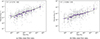 |
Fig. C.1. Flow rate versus core mass relation for only the flow rates closer to the core (panel (a)) and only the flow rates further from the core (panel (b)). |
Appendix D: Source and core parameters
Table of source parameters (ten-row preview).
Table of core parameters (ten-row preview).
All Tables
All Figures
|
Fig. 1. Source distribution for the regions in our ALMAGAL sub-sample is shown as black dots. The size of the markers scales with the masses of the ALMAGAL clumps. Grey dots are the rest of the ALMAGAL survey and the dashed line is a heliocentric distance circle at 5 kpc. |
| In the text | |
|
Fig. 2. Colour-coding for both figures is on evolutionary stage, legend shown in panel a. These plots show the sample of 17 quiescent, 23 protostellar, 22 YSO, and 25 HII regions. (a) Stacked histogram distribution of the luminosity-to-mass ratio for the regions in the ALMAGAL sub-sample being used for this work. (b) Individual cumulative distribution functions (CDF) of regions in each evolutionary stage, generated from kernel density estimates (KDEs) of the data shown in (a). |
| In the text | |
|
Fig. 3. Continuum image of ALMAGAL source AG348.5792–0.9197 from the astrodendro package where the green contours indicate the ‘leaves’ that are the areas we focus on here, namely: the cores. |
| In the text | |
|
Fig. 4. Zeroth moment map of SO (65–54) in grey-scale for source AG348.5792–0.9197 overlaid with continuum contours in black (levels 3, 6, 9σcont). A green star to show the peak intensity position of the core. Red and blue contours show the ‘wings’ of the spectral line emission, from 3 to 20 km s−1 either side, with respect to the region velocity of rest. |
| In the text | |
|
Fig. 5. Velocity analysis of source AG348.5792–0.9197. (a): First-moment map of YSO source AG348.5792–0.9197 in H2CO (30, 3–20, 2). The position of the continuum peak flux density is shown by the green star, and continuum contours are shown in black (levels 3, 6, 9σcont). The red line indicates the axis along which the PV cut was taken. (b): PV cut with 3 and 5σline contours in white, and the vlsr of the region shown by the white dashed line. The orange points show the nearest pixels at the 3σline contours. The red boxes are examples of the areas where we estimate the flow rates across (∼1″). The peak flux density position of the continuum core is located at the centre of each axis. |
| In the text | |
|
Fig. 6. Herschel derived dust temperature and the gas temperature plot against each other colour-coded in evolutionary stage. The grey dashed line shows the temperature equivalence line between the dust and the gas temperatures. |
| In the text | |
|
Fig. 7. Theoretical spreading of the observed flow rate due to unknown inclination of the filament for a tube-like cylindrical filament model with a universal flow rate of |
| In the text | |
|
Fig. 8. Histograms of the flow rate results for cores in each evolutionary stage quiescent to HII region from top to bottom. The mean and median are shown by the black dashed and grey solid lines, respectively, in each panel. |
| In the text | |
|
Fig. 9. Histograms of the flow rate results in the context of offset from the core. The top panel shows the results from the inner regions and the bottom from those further from the core. |
| In the text | |
|
Fig. 10. A histogram showing the distribution of the difference between the inner and outer flow rates per core ( |
| In the text | |
|
Fig. 11. Scatter plot of the results of the whole sample showing flow rate vs. core mass in grey. The purple points are the average flow rate/mass values per bin, with the associated errors. Here, each bin contains the same number of cores. A line of best fit is shown in black. |
| In the text | |
|
Fig. A.1. Histograms comparing the all regions in the ALMAGAL survey versus those ones chosen for this sample for distance, mass, luminosity, and L/M. |
| In the text | |
|
Fig. C.1. Flow rate versus core mass relation for only the flow rates closer to the core (panel (a)) and only the flow rates further from the core (panel (b)). |
| In the text | |
Current usage metrics show cumulative count of Article Views (full-text article views including HTML views, PDF and ePub downloads, according to the available data) and Abstracts Views on Vision4Press platform.
Data correspond to usage on the plateform after 2015. The current usage metrics is available 48-96 hours after online publication and is updated daily on week days.
Initial download of the metrics may take a while.