| Issue |
A&A
Volume 690, October 2024
|
|
|---|---|---|
| Article Number | A131 | |
| Number of page(s) | 22 | |
| Section | Numerical methods and codes | |
| DOI | https://doi.org/10.1051/0004-6361/202346798 | |
| Published online | 02 October 2024 | |
Predicting stellar rotation periods using XGBoost
1
Institut d’Estudis Espacials de Catalunya (IEEC),
08860
Castelldefels (Barcelona),
Spain
2
Departamento de Ciências de Computadores, Faculdade de Ciências, Universidade do Porto,
rua do Campo Alegre s/n,
4169-007
Porto,
Portugal
3
Faculty of Computer Science, Dalhousie University,
6050 University Avenue,
PO BOX 15000,
Halifax,
NS B3H 4R2,
Canada
4
Institute of Space Sciences (ICE-CSIC),
Campus UAB, Carrer de Can Magrans s/n,
08193,
Barcelona,
Spain
5
INAF, Osservatorio Astrofisico di Catania,
via Santa Sofia, 78
Catania,
Italy
6
LIAAD INESC Tec, INESC,
Campus da FEUP, Rua Dr. Roberto Frias,
4200-465
Porto,
Portugal
★ Corresponding author; This email address is being protected from spambots. You need JavaScript enabled to view it.
Received:
2
May
2023
Accepted:
18
June
2024
Abstract
Context. The estimation of rotation periods of stars is a key challenge in stellar astrophysics. Given the large amount of data available from ground-based and space-based telescopes, there is a growing interest in finding reliable methods to quickly and automatically estimate stellar rotation periods with a high level of accuracy and precision.
Aims. This work aims to develop a computationally inexpensive approach, based on machine learning techniques, to accurately predict thousands of stellar rotation periods.
Methods. The innovation in our approach is the use of the XGBoost algorithm to predict the rotation periods of Kepler targets by means of regression analysis. Therefore, we focused on building a robust supervised machine learning model to predict surface stellar rotation periods from structured data sets built from the Kepler catalogue of K and M stars. We analysed the set of independent variables extracted from Kepler light curves and investigated the relationships between them and the ground truth.
Results. Using the extreme gradient boosting (GB) method, we obtained a minimal set of variables that can be used to build machine learning models for predicting stellar rotation periods. Our models have been validated by predicting the rotation periods of about 2900 stars. The results are compatible with those obtained by classical techniques and comparable to those obtained by other recent machine learning approaches, with the advantage of using fewer predictors. When restricting the analysis to stars with rotation periods of less than 45 d, our models are on average wrong less than 5% of the time.
Conclusions. We have developed an innovative approach based on a machine learning method to accurately fit the rotation periods of stars. Based on the results of this study, we conclude that the best models generated by the proposed methodology can compete with the latest state-of-the-art approaches, while offering the advantage of being computationally cheaper, easy to train, and reliant only on small sets of predictors.
Key words: methods: data analysis / methods: miscellaneous / methods: statistical / stars: activity / stars: low-mass / stars: rotation
Deceased on 11 April 2023.
© The Authors 2024
 Open Access article, published by EDP Sciences, under the terms of the Creative Commons Attribution License (https://creativecommons.org/licenses/by/4.0), which permits unrestricted use, distribution, and reproduction in any medium, provided the original work is properly cited.
This article is published in open access under the Subscribe to Open model. This email address is being protected from spambots. You need JavaScript enabled to view it. to support open access publication.
1 Introduction
Measuring the rotation of stars is an essential field of stellar astrophysics. One of the main methods for quantifying the rotation periods of stars is to analyse their light curves and look for modulations that can be related to the stellar rotation rate. Solartype stars, namely, low-mass stars with convective outer layers, are known to develop spots on their surfaces. The origin of these spots is related to stellar magnetism (e.g. Brun & Browning 2017). Similarly, high-mass (e.g. Cantiello & Braithwaite 2011) and fully convective low-mass stars (e.g. Bouvier & Bertout 1989; Damasso et al. 2020; Bicz et al. 2022) also exhibit magnetic spots on their surfaces. Such spots can induce a modulation in stellar light curves which, in principle, allows for the determination of both stellar rotation periods and long-term stellar magnetic activity cycles (e.g. Strassmeier 2009). The rotation period of a star is essential for understanding the transport mechanisms related to the stellar angular momentum, a process that is still poorly understood (Aerts et al. 2019) but especially important for obtaining correct age estimations for stars (Eggenberger et al. 2009). The latter can be very important for the characterisation of planetary systems (Huber et al. 2016). The role of stellar rotation in driving stellar dynamos and determining magnetic cycles is also still much debated (e.g. Bonanno & Corsaro 2022). Any theory on this subject requires an accurate calculation of rotation periods for all types of stars.
The accuracy and precision with which stellar rotation is measured are crucial for the study of stellar evolution. The rotation period of a star correlates with its age: solar-type stars are known to spin down during their main-sequence evolution and so, the rotation period of young solar-like stars can be used to constrain stellar ages using ‘gyrochronology relations’ (Barnes 2003; Skumanich 1972; García et al. 2014; Messina 2021; Messina et al. 2022). However, for stars older than the Sun, gyrochronological ages are not in agreement with asteroseismic ages (Van Saders et al. 2016; Hall et al. 2021) and those inferred from velocity dispersion (Angus et al. 2020). In this case, such a discrepancy can only be solved by developing new methods for accurately measuring stellar rotation.
The vast amount of astronomical photometric data released over the last three decades has recently motivated the use of machine learning (ML) techniques to process and analyse them.
The advent of new large-scale sky surveys and the need to process large numbers of targets simultaneously make manual handling astrophysical data impractical, while the use of artificial intelligence (AI) techniques is becoming increasingly popular (e.g. Pichara Baksai et al. 2016; Biehl et al. 2018). A stellar light curve is nothing more than a time series of photometric data from a star, namely, a sequence of stellar surface fluxes collected at successive points in time. The last decade has seen the emergence of many observations that provide high- quality, long-term and near-continuous stellar photometric data. Examples include the Kepler space observatory (Borucki et al. 2009) and the reborn Kepler K2 mission (Howell et al. 2014), which have altogether observed more than half a million stars (Huber et al. 2016)1. Furthermore, Transiting Exoplanet Survey Satellite (TESS, Ricker et al. 2014) has collected light curves with time spans of 25 d to one year for tens of millions of stars. Such a large number of observations requires automated procedures to process and extract information from them and machine learning methods can be used to accomplish this goal.
The first step in choosing an ML technique is to select the data from available sources and study them carefully. Typically, two approaches can be adopted: using the photometric time series data directly as input or first converting the light curves into structured data that can be represented by a set of variables or features in tabular form. Machine learning models can be trained from these two types of data (unstructured and structured), automating processes that would otherwise be tedious or require too much human effort.
The first case (i.e. unstructured data) is usually tackled with special types of artificial neural networks (ANN, Haykin 2009), which are reinforcement algorithms that require little or no pre-processing of the data. Blancato et al. (2022) used a deep learning (DL) approach and applied convolutional neural networks (CNNs) to predict stellar properties from Kepler data. Claytor et al. (2022) applied a CNN to synthetic light curves to infer stellar rotation periods and then estimated the rotation periods of 7245 main-sequence TESS stars, with periods up to 35 d for G and K dwarfs and up to 80 d for M dwarfs (Claytor et al. 2024). This was achieved using a CNN, which allowed the light curve systematics related to the telescope’s 13.7-day orbit to be removed. However, training neural networks typically requires large computational resources.
The second scenario (i.e.using structured data) is resolved by resorting to algorithms that use tabular data to perform unsupervised (clustering) and supervised (classification and regression) tasks. Lu et al. (2020) developed a model that predicts the rotation periods of TESS stars with an uncertainty of 55%, by training a random forest (RF, Breiman 2001) regressor on Kepler data. The most important features for predictions in their model were the range of variability in the light curve, effective temperature, Gaia colour, the luminosity, and the brightness variation on timescales of 8 h or less. Breton et al. (2021) applied RFs to tabular Kepler data to produce three ML classifiers that can detect the presence of rotational modulations in the data, flag close binary or classical pulsator candidates, and provide rotation periods of K and M stars from the Kepler catalogue (Brown et al. 2011). The method was then applied to F and G main- sequence and cool subgiant Kepler stars by Santos et al. (2021). Breton et al. (2021) used 159 different inputs to train the classifiers: rotation periods, stellar parameters (e.g.mass, effective temperature, and surface gravity), and complementary variables obtained from wavelet analysis, the autocorrelation function of light curves and the composite spectrum. The authors claimed accuracies of 95.3% (when accepting errors within 10% of the reference value) and of 99.5% after a visual inspection of 25.2% of the observations. Breton et al. (2021) used a classification approach, namely, their algorithm was trained to select the most reliable rotation period among these candidate values. One particularity of their work is that they used rotation periods as input variables for training their models. We expected these features to be highly correlated with the response or target variable (the rotation periods considered as ground truth). Thus, we decided to (i) explore their data set and determine what is this level of correlation and (ii) try to train ML models without these rotation period input variables to compare the performance of our models with theirs.
In this paper, we focus on the prediction of rotation periods of K and M stars from the Kepler catalogue (Borucki et al. 2009, 2010), using an ML method. We follow a regression-based approach, namely, we propose predicting the rotation period of several targets, rather than selecting the best candidate among some previously computed values, as in a classification problem. We also address the selection of suitable data, the size of the data set, the optimisation of the ML model parameters, and the training of the latter. The time and computational resources were also important constraints in the development of this project, especially during the learning phase of the models.
The paper is structured as follows: in Sections 2 and 3, we describe the data and the methods used for the experiments. In Sect. 4, we present a discussion of our experimental design. In Sect. 5, we present the results of our contributions by applying a supervised ML approach to predict the rotation periods of stars. In Sect. 6 is dedicated to the discussion of the results and we summarise our contributions in Sect. 7.
2 Materials
The main objective of this project is to develop robust, yet computationally inexpensive supervised ML models from tabular astronomical data for the prediction of stellar rotation periods of K and M stars from the Kepler catalogue.
We used sets of structured, tabular data, containing measurements for the features or predictors and for the response or target variable. Computationally, these tabular data have been organised into data frames, where the columns correspond to the variables (predictors plus response) and the rows correspond to the observations. Each of the rows, consisting of measurements for one star, will be referred to as an observation, an instance, a case, or an object.
These data sets were divided into training and testing sets. The former were used to build prediction models or learners, which, in turn, were used to predict the rotation period of unseen stars, provided they were input as structured data sets similar to the training set, namely, in tabular form, containing at least some of its features. The testing sets acted as the never-before-seen objects, with the advantage of containing the outcome (not given to the model), which could be used to assess the predictive performance and quality of the models by comparing the predicted values with the true outcomes or ground truth. We considered a good model to be one that accurately predicts the response. The following sections describe the specific materials and methods used to build the models and assess their performance2.
2.1 Description of the data
We focused on real data, including features extracted from the light curves, and “standard” predictors, namely, variables that are commonly obtained directly or indirectly from astronomical observations.
We started by analysing structured data from the Kepler catalogue of K and M dwarf stars, already in tabular form, published by Santos et al. (2019) and Breton et al. (2021), whose targets were selected from the Kepler Stellar Properties Catalogue for Data Release 25 (Mathur et al. 2017). Both catalogues (hereafter referred to as S19 and B21, respectively) contain all the predictors and targets considered in our work: B21 was used as the source for most of the predictors; S19 was used specifically to extract the rotation periods and features obtained directly from Kepler observations. The latter are commonly known as ‘stellar parameters’ in the astronomical community and examples include the mass of the star and its effective temperature. However, we do not use the word ‘parameter’ in this context to avoid confusion with the model parameters. Instead, we will use the terminology of astrophysical variables when referring to them.
B21 is available in tabular form, without any particular clustering or classification of the variables. However, we decided to group the predictors according to their nature and/or the method by which they were obtained. We have identified six groups whose characteristics are described in the following paragraphs3.
Astrophysical. (Astro, astro) – predictors related to the physical properties of the stars, derived directly or indirectly from the observation: (i) effective temperature, Teff (teff), and its corresponding upper and lower errors,  (teff_eup) and
  (teff_elo) respectively; (ii) the logarithm of the surface gravity, log 𝑔 (logg) and its upper and lower error limits, log gerr, up (logg_eup) and log 𝑔err,low (logg_elo); (iii) the mass of the star, M (m), and its upper and lower errors, Merr, up (m_eup) and Merr,low (m_elo); (iv) the magnitude from the Kepler input catalogue, Kp (kepmag); and (v) the Flicker in power (FliPer) va lues, F0.7 (f_07), F7 (f_7), F20 (f_20), and F50 (f_50), respectively corresponding to cut-off frequencies of 0.7, 7, 20 and 50 µHz.
Time series. (TS, ts) – quantities that are related to the properties of the time series: (i) the length of the light curve in days, l (length); (ii) the start and end times of the light curve, St (start_time) and Et (end_time) respectively; (iii) the number of bad quarters in the light curve, nQbad (n_bad_q); (iv) the photometric activity proxy or index, Sph (sph), and its error,  (sph_e), according to Santos et al. (2019); (v) the photometric activity proxy computed from the autocorrelation function (ACF) method to obtain the rotation period,
  (sph_acf_xx), for each of the xx-day filters, where xx ∈ {20, 55, 80}, as provided by Breton et al. (2021), and its corresponding error,
  (sph_acf_err_xx)4; (vi) the height of the PACF (i.e.the period of the highest peak in the ACF at a lag greater than zero), GACF (g_acf_xx), for each of the xx-day filters; and (vii) the mean difference between the heights of PACF at the two local minima on either side of PACF, HACF (h_acf_xx), for each of the above filters.
Global wavelet power spectrum. (GWPS, gwps) – quantities obtained from a time-period analysis of the light curve using a wavelet decomposition: (i) the amplitude (gwps_gauss_1_j_xx), central period (gwps_gauss_2_j_xx), and standard deviation (gwps_gauss_3_j_xx) of the jth Gaussian fitted to the GWPS with the xx-day filter, for j ∈ {1, 2, …, 6}; (ii) the mean level of noise of the Gaussian functions fitted to the GWPS for the xx-day filter (gwps_noise_xx); (iii) the χ2 of the fit of the Gaussian function to GWPS for the xx-day filter (gwps_chiq_xx); (iv) the number of Gaussian functions fitted to each GWPS for the xx-day filter (gwps_n_fit_xx); and (v) the photmetric proxy computed from the GWPS method,  (sph_gwps_xx), as provided by Breton et al. (2021), and its corresponding error,
  (sph_gwps_err_xx).
Composite spectrum. (CS, cs) – variables obtained from the product of the normalised GWPS with the ACF: (i) the amplitude of the PCS (the period of the fitted Gaussian with the highest amplitude), HCS (h_cs_xx), for the xx-day filter; (ii) the average noise level of the Gaussian functions fitted to the CS, csnoise (cs_noise_xx), for the xx-day filter; (iii) the χ2 of the fit of the Gaussian function to the CS for the xx- day filter (cs_chiq_xx); (iv) the photometric proxy computed by the CS method,  (sph_cs_xx), and its error,
  (sph_cs_err_xx) for the xx-day filter; and (v) the amplitude (cs_gauss_1_j_xx), central period (cs_gauss_2_j_xx), and the standard deviation (cs_gauss_3_j_xx) of the jth Gaussian fitted to the CS with the xx-day filter, for j ∈ {1, 2, … , 6}.
Rotation periods. (Prot, prot) – rotation periods obtained by combining the ACF, CS, and GWPS time-period analysis methods with the KEPSEISMIC light curves, for the x x-day filters:  (prot_acf_xx),
  (prot_cs_xx), and
  (prot_gwps_xx)5.
The list of 170 explanatory variables, as they appear in the final data set after exploratory data analysis, cleaning, and engineering, is referenced in Table 1. In total, there are 14 Astro, 18 TS, 66 GWPS, 63 CS, and nine Prot predictors.
We chose to use previously published real-world data because they are readily available and our aim is to compare distinct machine learning approaches using different sets of predictors; thus, we want to analyse how much the predictions are affected by the variables closely related to the method used to estimate the reference rotation periods. Also, comparisons of the results with the state-of-the-art can only be made fairly if the data sets are built from the same reference set of observations.
In the following section, we describe the steps we applied to S19 and B21 to build a master data set and several subsets which we used to build the ML models.
Names of the 170 predictors, as they appear in the original data set, and their description.
2.2 Data engineering
The data from S19 and B21 were cleaned and merged to create a master data set, from which several subsets were generated. During the cleaning process, (i) columns containing only null values were dropped, (ii) rows with less than 5% of non-null predictors were removed, (iii) rows containing extreme standard deviation values were removed, (iv) very extreme values of variables other than standard deviations were flagged as NaN and subsequently imputed, (v) rows corresponding to targets with rotation errors greater than 20% of the respective rotation period were removed, (vi) flag-type variables from S19 and B21 were dropped, (vii) all variable names were converted to lowercase, and (viii) some names were changed, for clarity.
In the merging process, we selected all stars that were present simultaneously in both data sets. As explained in detail in Sect. 3.1, we chose to use the XGBoost (XGB) version of the tree-based ensemble approach known as gradient boosting (GB) to train our models. Missing values were imputed using a random forest (RF) with 500 trees and a sample fraction of 0.5. Following data imputation, we decided to create a parallel data set with standardised predictors for further analysis. We note that because we used a tree-based (as opposed to a distance-based) ensemble method, normalisation of the predictors would not be strictly required (Murphy 2012; Chen & Guestrin 2016). Nevertheless, since XGBoost uses a gradient descent algorithm, we decided to use the normalised version of the data set to create the subsets from which the XGB models would be built, in order to optimise the computations during the training phase.
Several features, mainly in the CS and GWPS groups (recall the group in variables in the previous section), exhibit values with extremely large or infinite amplitudes. They are derived variables, corresponding to some of the amplitudes, central periods, standard deviations, and mean noise levels of the Gaussian functions fitted to the CS and GWPS. Their extreme values may have different origins, such as instrumental errors, and possibly they may have been taken into account when they were created. In principle, the presence of outliers would not be a problem, as there are no restrictions on extreme points in GB, and XGB can handle missing values. However, as we are validating a methodology and want to leave open the possibility of comparing the performance of XGBoost with other methods that cannot handle missing values (such as some implementations of RFs), we chose to flag these outliers as missing values and subsequently impute them. We note that the main data set still contains large values from which the models could learn.
After the aforementioned transformations, we ended up with a data set containing 14 913 observations and 170 predictors. This is the full or master set, labelled Data Set 0 (DS0). Several subsets were created from the full data set, each containing a different number of predictors and/or instances: (i) the first subset was obtained by removing the nine rotation period variables (Prot group) and the six *_gauss_2_1_* predictors (GWPS and CS groups), resulting in a data set of 155 independent variables; this is referred to as Data Set 1 (DS1); (ii) a second subset was created by removing from DS1 redundant variables, correlated between them, resulting in a data set with 146 predictors – Data Set 2 (DS2); (iii) the third subset was obtained from DS2, by removing stars with surface rotation periods greater than 45 d, leaving a data set of 14356 rows - this is Data Set 3 (DS3); (iv) the fourth subset is obtained by removing from DS3 stars with surface rotation periods less than 7 d, resulting in a data set of 13 602 rows – Data Set 4 (DS4); (v) a fifth subset was built on top of DS3, using the twenty-eight most important variables as assessed by the previous models – Data Set 5 (DS5); (vi) a sixth subset was obtained from DS4, using the twentyeight most important variables as scored by the models built with DS0 to DS4 – Data Set 6 (DS6); (vii) a final subset was created from DS1, where we used the same twenty-eight most important variables used to build DS5 and DS6 – Data Set 7 (DS7).
In the process of constructing DS1, we observed a single instance in which the reference rotation period did not align with any of the *_gauss_2_1_* predictors. Additionally, a small number of instances (fewer than 10 out of 14 913 cases) were identified where the values of the gwps_gauss_2_2_80 or gwps_gauss_2_3_55 variables were equal to the reference value. However, in those instances, the values of at least one of the *_gauss_2_1_* variables coincided with the reference value. Consequently, we proceeded to eliminate the central period (i = 2) of the first Gaussian (j = 1) fitted in the CS and GWPS. This procedure was implemented in order to ensure that the rotation period values had been removed from the predictors and would not influence the subsequent training of the models.
DS2 was constructed by performing a simple univariate filtering of the features, where the predictors were crossvalidated with the response variable in order to remove redundant or uninformative variables from the learning process. The analysis of correlations between variables is detailed in Sect. 2.3.
DS3 was built because of Kepler’s 90-day quarters (Mullally 2020), to ensure at least two full cycles of observations per object, thus preventing any problems that may arise from stitching together data from different quarters and other potential long-term issues related to the telescope, such as those related to Kepler’s orbital period and its harmonics. Although Breton et al. (2021) have identified and distinguished rotating stars from other types of objects, we also removed stars with surface rotation periods less than 7 d, because these targets can easily be mistaken for close-in binary systems, classical pulsators, or other false positives, whose signals may mimic stellar objects manifesting surface rotation, and we wanted to check how the model would behave by removing these potentially misclassified targets. By including only stars with rotation periods between 7 d and 45 d, as we did in DS4, we expected to improve the predictive performance of the models. We ended up with 13 602 stellar objects, a reduction of about 9% compared to the DS0, DS1, and DS2 data sets.
We also selected the top 20 most important variables in the models trained with the data sets DS0 to DS4, and took their union. This resulted in a set of 28 predictors, which we used to build DS5, DS6, and DS7. These three data sets contain only the most important features identified during the learning of the previous XGB models.
2.3 Statistical analysis of relevant variables
All variables present in DS0, including the response, prot (the stellar rotation period, in days), are continuous. The histograms and box-plots of the target variable, as extracted from DS0 (top panels) and its training set (bottom panels), are shown in Fig. 1. The sample distributions are very similar to each other. The aforementioned plots suggest unimodal, slightly platykurtic, and right-skewed distributions, with several outliers towards large quantiles, corresponding to the largest stellar rotation periods, above approximately 50 d up to about 100 d. The medians are equal to 23.87 d, with minima and maxima of 0.53 d and 98.83 d, respectively. The histograms show that the majority of the stars in the sample have rotation periods roughly between zero and 50 d, but the right tail of the distributions extends well beyond this interval. Therefore, there is no statistical evidence of uniformity in the distribution of prot.
Figure 2 is similar to Fig. 1, but for DS4. The distributions on the full and training sets are very similar to each other. There is no statistical evidence of uniformity in either set, although the distributions are flatter than their DS0 counterparts. The plots suggest unimodal, platykurtic, slightly right-skewed distributions. For both DS4 and its training set, the median is 24.03 d and the minimum and maximum are 7.00 d and 44.85 d, respectively; the mean is equal to 24.42, and the standard deviations are 9.10 d and 9.12 d, respectively. From the histograms, we can see that the sample lacks stars with rotation periods of up to about 12 d and above about 32 d. The fact that the distribution of prot is not uniform affects the learning of the models, especially in the less represented regions.
In DS0, after removing targets with rotation errors 20% larger than the corresponding rotation periods, as described in Sect. 2.2, the distribution of the rotation period errors ( , Fig. 3) is unimodal, right skewed, and slightly platykurtic. The errors vary between 0.03 d and 13.19 d, with a median of 1.92 d. The outliers indicated by the box-plot are not significant, as all the errors are less than 20 % of their corresponding rotation periods. A significant number of points in the QQ-plot are outside the 95 % confidence band, and the graph has two pronounced tails. Therefore, there is no statistical evidence of normality in the distribution of
  .
.
The scatter plot of the rotation period errors as a function of the rotation periods is illustrated in Fig. 4. The majority of the measurements correspond to targets with rotation periods of less than 50 d. Two branches can be identified, one starting at the lowest rotation periods and another starting at prot ≃ 10 d. The nature of these branches is not known. Both branches show a linear relationship between  and prot without much dispersion up to a certain rotation period of about 10 d on the upper branch and 27 d on the lower branch. Beyond these limits, the dispersion increases with prot. The upper branch goes up to the maximum values of prot, while the lower branch stops at about 55 d. An outlier at prot = 82 d seems to belong to the lower branch, but as with the branches, its nature is unknown. For rotation periods of around 50 d, the amplitude of the dispersion in the upper branch is about 7 d. Increasing dispersion with prot can lead to a decrease in model performance and be a source of outliers in the predictions.
The correlations between the Prot, TS, and Astro families of variables and the response are shown in Figs. 5–7. The correlation between some of the variables belonging to the CS and GWPS families and the Astro group and Prot is shown in Figs. A.1 and A.2. Reddish colours indicate a positive correlation between any two features, blueish colours indicate a negative correlation, and white indicates no correlation at all. As expected, most of the Prot variables are strongly positively correlated with the response, since the latter is obtained directly from the estimation of the former. The same can be said of the variables containing the central period of the first Gaussian function fit in the CS and GWPS (although they are not represented in the correlation plots above). These variables were the source of the values of the ground truth, and therefore also exhibit a strong positive correlation with it. This was the motivation for creating the DS1 data set. Some of the TS features are negatively correlated with the response (Fig. 6), such as h_acf_20, g_acf_20, or sph_acf_20. These predictors are expected to be important in building the models, as opposed to variables that have little correlation with prot, such as start_time, end_time, and n_bad_q. All TS variables extracted from the ACF are highly correlated with each other, which in principle is not a problem because we used tree-based ensembles (see Sect. 3.1). Classical ‘Astro’ variables are not correlated with the response (Fig. 7), apart from the mass, some cut-off frequencies of the Flicker in power (FliPer) method, and the effective temperature. However, some features of the CS and GWPS families, such as cs_gauss_, gwps_gauss_, and their errors, are strongly correlated with the FliPer metrics (Bugnet et al. 2018, see Figs. A.1 and A.2). This means that, in principle, any one of these variables could be replaced for the other without affecting how well the model performs. For the CS and GWPS families of variables, we identified three groups of correlation with the response: low correlation, strong positive, and strong negative correlation. Examples of strong positive correlations are cs_gauss_2_l_20, cs_gauss_3_l_20, and gwps_gauss_2_1_55, and examples of strong negative correlations are h_cs_20 and sph_gwps_20, just to name a few.
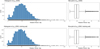 |
Fig. 1 Histograms (left panels) and box-plots (right panels) of the target variable, prot, on DS0 (top row) and on the training set generated from it (bottom row). The distributions are very similar to each other, right skewed, with medians equal to 23.87 d, minima and maxima of 0.53 d and 98.83 d, respectively. Both have several outliers. |
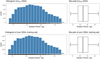 |
Fig. 2 Similar to Fig. 1, but for the DS4 data set. The distributions are very similar to each other, approximately symmetrical, with means of 24.44 d and 24.43 d, and standard deviations of 9.11 d and 9.07 d, on DS4 and its training set, respectively. |
 |
Fig. 3 Histogram (left panel), box-plot (middle panel), and QQ-plot (right panel) of the rotation period errors, |

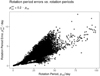 |
Fig. 4 Rotation period errors, |

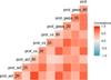 |
Fig. 5 Correlations between the Prot variables and the response. In this case, all predictors are highly correlated with the target variable. |
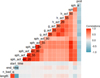 |
Fig. 6 Correlations between the TS variables and the response. |
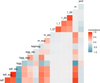 |
Fig. 7 Correlations between the ‘Astro’ variables and the response. |
3 Methods
3.1 Problem formulation
Stellar rotation periods are positive real numbers, that can range from almost zero up to tens or hundreds of days (e.g. Santos et al. 2019; McQuillan et al. 2014), and so we framed the problem as a regression task. Assuming that there is a relationship between a quantitative response y and a set of p predictors x = (x1, x2, …, xp), our problem can be described mathematically by the equation
 (1)
(1)
where f is an unknown fixed function of x, and e is a random error term independent of x, with zero mean. The function f can be estimated, but it is never fully known. If the inputs x are readily available, given an estimate for  , the output can be predicted by
 (2)
(2)
In the context of this project, the target variable y and the p predictors are the rotation period, prot, and the set of variables described in Sect. 2 and Table 1, respectively, so that Eq. (1) becomes
 (3)
(3)
In this equation, the index p is an integer that varies up to 170, according to the number of variables that make up the data set used to train the model (DS0 to DS7). The models, trained by ML methods, can be expressed generically as
 (4)
(4)
where  is the estimate of f. We were not concerned with the exact form of
  , but rather with the accuracy of the predictions made by the models.
An important condition for us was that the models should simultaneously be robust, have good predictive performance, and be computationally cheap. Given the tabular nature of the available data, we decided to use a tree-based ensemble method, specifically XGBoost, to tackle the research problem, as it is fast and has recently been shown to be the best for predictive tasks from structured data (Géron 2017; Raschka & Mirjalili 2017).
The proposed method aims to improve the predictive performance of existing models, such as the RF classifier published by Breton et al. (2021), so that rotation periods can be estimated for thousands of K and M stars from the Kepler catalogue, in an efficient and timely manner, with little human interaction.
3.2 The extreme gradient boosting approach
Boosting can combine several weak learners, namely, models that predict marginally better than random, to produce a strong model, an ensemble with a superior generalised error rate. The gradient boosting (GB) method (Friedman 2001) can be applied to classification and regression tasks, based on the idea of steepest-descent minimisation. Given a loss function L and a weak learner (e.g. regression trees), it builds an additive model as:
 (5)
(5)
which attempts to minimise L. In this equation, wk is the kth weight of the weak base model hk(xi), and xi is the predictor i, as defined in Sect. 3.1. The algorithm is typically initialised with the best estimate of the response, such as its mean in the case of regression, and it tries to optimise the learning process by adding new weak learners that focus on the residuals of the current ensemble. The model is trained on a set consisting of the cases (xi, ri), where ri is the ith residual, given by
 (6)
(6)
The residuals thus provide the gradients, which are easy to calculate for the most common loss functions. The current model is added to the previous one, and the process continues until a stopping-condition is met (e.g. the number of iterations, specified by the user).
We used XGBoost, a successful implementation of GB, which was designed with speed, efficiency of computing resources, and model performance in mind. The algorithm is suitable for structured data. It is able to automatically handle missing values, it supports parallelisation of the tree-building process, it automatically ensures early stopping if the training performance does not evolve after some predetermined iterations, and it allows the training of a model to be resumed by boosting an already fitted model on new data (Chen & Guestrin 2016). The method implements the GB algorithm with minor improvements in the objective function. A prediction of the response is obtained from a tree-ensemble model built from K additive functions:
 (7)
(7)
where the function fk belongs to the functional space ℱ of all possible decision trees. Each fk represents an independent tree learner. The final prediction for each example is given by the aggregation of the predictions of the individual trees. The set of functions in the ensemble is learned by minimising a regularised objective function,  , which consists of two parts:
 (8)
(8)
The first term on the right-hand side of Eq. (8) is the training loss,  , and the second term is the regularisation term. Here, ℓ is a differentiable convex loss function that measures the difference between the predicted and the true values of the response. The training loss measures how good the model is at predicting using the training data, and it may be selected from a number of performance metrics, some of which will be described in detail in Sect. 3.3. The regularisation term controls (penalises) the complexity of the model. It helps to smooth the final learning weights, to avoid overfitting. In practice, the regularised objective function tends to select models that use simple and predictive functions (Chen & Guestrin 2016). A model is learned optimising the objective function above.
The XGBoost algorithm has several hyperparameters, which are not considered in Eq. (4). Hyperparameters are tuning parameters that cannot be estimated directly from the data, and that are used to improve the performance of an ML model (Kuhn et al. 2013). They are parameters of a learning algorithm, not of a model, and are mostly used to control how much of the data is fitted by the model, so that, ideally, the true structure of the data is captured by the model, but not the noise. Optimising them using a resampling technique is crucial and the best way to build a robust model with good predictive performance. They are set in advance and remain constant throughout the training process. Hyperparameters are not affected by the learning algorithm, but they do affect the speed of the training process (Géron 2017; Raschka & Mirjalili 2017). There is no formula for calculating the optimal value nor a unique rule for tuning the parameters used to estimate a given model. The optimal configuration depends on the data set, and the best way to build a model is to test different sets of hyperparameter values using resampling techniques. Section 4 describes the strategy we used to optimise the XGBoost hyperparameters.
3.3 Performance assessment
The performance of the ML models built with the data sets described in Sect. 2.2 was assessed by quantifying the extent to which the predictions were close to the true values of the response for the set of observations. Given the regression nature of the problem in this project, we used six metrics to assess the predictive quality and the goodness of fit of the learners: (a) the root mean squared error (RMSE) and the mean absolute error (MAE); (b) an interval-based error or residual, ϵ∆,δ: (c) an interval-based ‘accuracy’, acc∆, calculated using the interval-based error; (d) the mean of the absolute values of the residuals, µerr; and (e) the adjusted coefficient of determination,  . Furthermore, the error bars associated with the predictions were estimated in accordance with the specifications outlined in Sect. 3.3. The RMSE, MAE, and ϵ∆,δ were used to measure the statistical dispersion, while acc∆ and
  were used to assess the predictive performance of the models. The mean of the residuals, µerr, was used simultaneously as a measure of the dispersion and of the quality of the models, in the sense that we could infer from it how wrong the models were on average.
During the learning phase, a model’s performance was estimated using the k-fold cross-validation (CV), where a subset of observations was used to fit the model, and the remaining instances were used to assess its quality. This process was repeated several times, and the results were aggregated and summarised.
After the training phase, predictions were made on each of the testing sets, and the resulting rotation periods were compared with the reference values contained in the S19 catalogue. The mean of the relative absolute values of the residuals was used as a measure of goodness of fit, giving us an idea of how wrong the models were on average. The RMSE and the MAE were used together to measure the differences between the predicted and reference values of stellar rotation periods. They were particularly useful in assessing the performance of the models on the training and testing sets, and thus to better tuning them in order to avoid overfitting – large differences in the RMSE and/or MAE between the training and testing sets are usually an indication of overfitting. The interval-based accuracy allowed us to convert the assessment of a regression problem into the evaluation of a classification result. This in turn allowed us to compare the predictive performance of our models with those trained by Breton et al. (2021). Since the latter assessed their results within a 10% interval of the reference values, we used the 10%-accuracy, acc0.1, as a benchmark. When calculating the interval accuracies, it should be noted that the width of the intervals centred on the reference values increases with the rotation period, while the width of the intervals around the corresponding rotation frequencies does not vary significantly with the frequency, except in the low-frequency range. Since the distribution of the amplitudes of the frequency intervals is more uniform than that of the amplitudes of the period intervals, the rotation periods were first converted to rotation frequencies in order to reduce the effect of the increasing width of the accuracy intervals with the period, which would affect the comparisons and the assessment of the quality of the models. The following is a brief description of each of the above metrics and the k-fold CV technique.
RMSE. The most commonly used metric to assess the performance of a model in a regression setting is the mean squared error (MSE). This is defined as:
![Mathematical equation: ${\rm{MSE}} = {1 \over n}\sum\limits_{i = 1}^n {\left[ {{{\left( {{y_i} - {{\hat y}_i}} \right)}^2}} \right]} ,$](/articles/aa/full_html/2024/10/aa46798-23/aa46798-23-eq35.png) (9)
(9)
where  is the prediction for the ith observation given by
  , and n is the number of cases present in the data set. The MSE is a measure of the distance between a point estimator
  and the real value or ground truth y. It is usually interpreted as how far from zero the errors or residuals are on average, i.e. its value represents the average distance between the model predictions and the true values of the response (Kuhn et al. 2013). In general, a smaller MSE indicates a better estimator (Ramachandran & Tsokos 2020): the MSE will be small when the predictions and the responses are slightly different, and will typically be large when they are not close for some cases. The MSE can be computed on both the training and testing data, but we are mostly interested in measuring the performance of the models on unseen data (the testing sets); thus, the model with the smallest testing MSE has the best performance. If a learner produces a small training MSE but a large testing MSE, this is an indication that it is overfitting the data, and therefore a less flexible model would produce a smaller testing MSE (James et al. 2013). A common measure of the differences between estimates and actual values is the root mean squared error (RMSE), which is no more than the square root of the MSE:
 (10)
(10)
The RMSE has the advantage over the MSE that it has the same units as the estimator. For an unbiased estimator, it is equal to the standard deviation. Similarly to the MSE, smaller values of the RMSE generally indicate a better estimator, but as this metric is dependent on the scale of the variables used, comparisons are only valid between models created with the same data set (Hyndman & Koehler 2006).
MAE. The mean absolute error (MAE) of an estimator  is the average of the absolute values of the errors:
 (11)
(11)
where all of the quantities have the same meaning as before. The MAE is a measure of the error between the prediction and the ground truth. It uses the same scale as the estimates and the true values. Therefore, it cannot be used to make comparisons between models built on different data sets. The MAE has the advantage over the RMSE that it is affected by the error in direct proportion to its absolute value (Pontius et al. 2008). When used together, the RMSE and MAE can diagnose variations in the residuals in a set of predictions. For each predictive model and sample under consideration,
 (12)
(12)
The variance of the individual errors increases with the difference between the RMSE and the MAE, and all the errors are of the same size when both metrics are equal to each other.
MARE. The mean absolute value of the relative error (MARE) is given by
 (13)
(13)
where n is the number of observations, yi = f (xi) and  . It is similar to the MAE, but the mean absolute value is calculated on the relative residuals rather than the magnitude of the errors. The MARE is a measure of the model’s mean relative error, giving a percentage estimate of how wrong the model is on average.
Interval accuracy. We developed an interval-based error function and an “accuracy” metric to bridge the gap between regression and classification settings. The interval-based error, ϵ∆,δ, estimates the prediction error in a regression task when we are willing to accept an error of 100 × ∆%, and it is given by:
![Mathematical equation: ${_{\Delta ,\delta }} = \left\{ {\matrix{ {0,} \hfill & {\left| {{_i}} \right|\Delta \cdot {y_i}} \hfill \cr {\left[ {(1 + \Delta ) \cdot {y_i} - {{\hat y}_i}} \right]{{1 + \delta } \over \delta },} \hfill & {\Delta \cdot {y_i} < {_i}\Delta \cdot (1 + \delta ){y_i}} \hfill \cr {\left[ {(1 - \Delta ) \cdot {y_i} - {{\hat y}_i}} \right]{{1 + \delta } \over \delta },} \hfill & { - \Delta \cdot (1 + \delta ){y_i}{_i} < - \Delta {y_i}} \hfill \cr {{_i},} \hfill & {{\rm{ otherwise, }}} \hfill \cr } } \right.$](/articles/aa/full_html/2024/10/aa46798-23/aa46798-23-eq45.png) (14)
(14)
where  and
and  are the ith ground truth and predicted values, respectively, ∆ is the fractional width of the zeroing interval, and δ is the fraction of ∆ · y that defines a transition zone, where the error varies linearly between zero and the typical residual. When ∆ is zero, the metric returns the simple residuals. The second and third branches of Eq. (14) correspond to the transition zone. We used a linear function to join the residuals to the error interval, but any other function could be used, such as a logistic function or a hyperbolic tangent, just to name a few. Figure 8 shows the interval-based error function calculated on simulated data, when an error of 10% is considered acceptable, i.e. when ∆ = 0.1. The transition zone is defined for δ = 0.2, corresponding to 20 % of ∆ · y. The predictions were obtained from a uniform distribution of 200 values varying between 0 and 2 around a fixed ground truth value of 10. Similar to Eq. (13), this error function, when normalised to the reference values, can be used to approximate how much a model is wrong on average for a given error-interval width.
An interval-based ‘accuracy’, acc∆, can be obtained from the interval-based residuals of Eq. (14):
 (15)
(15)
where ∆, yi, and  are as before, and n is the number of observations6. The indicator function is equal to 1 when the interval-based regression error is zero, namely, whenever
  , and zero otherwise; that is, we consider an event every time the error in Eq. (14) is equal to zero, and a non-event otherwise.
Adjusted coefficient of determination. We used the adjusted coefficient of determination,  , as a fair measure of a model’s goodness of fit, to characterise its predictive ability:
 (16)
(16)
where R2 is the coefficient of determination, n is the number of observations, and p is the number of predictor variables (Baron 2019).
k-fold cross-validation. We used the k-fold cross-validation as a resampling technique during the training phase of the models, in which the training instances were randomly partitioned into k non-overlapping sets or folds of approximately equal size. One of the folds was kept as the validation set, and the remaining folds were combined into a training set to which a model was fitted. After assessing the performance of the model on the validation fold, the latter was returned to the training set, and the process was repeated, with the second fold as the new validation set, and so on and so forth (Kuhn et al. 2013; Hastie et al. 2009). The k performance estimates were summarised with the mean and the standard error, and they were used to tune the model parameters. The testing error was estimated by averaging out the k resulting MSE estimates. The bias of the technique, namely, the difference between the predictions and the true values in the validation set, decreases with k. Typical choices for k are 5 and 10, but there is no canonical rule. Figure 9 illustrates an example of a CV process with k = 3.
Estimation of error bars. In order to estimate the errors associated with the predictions made on the testing set, we employed a straightforward methodology, whereby the predictions were binned into uniform unit intervals centred on integer values spanning between the minimum and the maximum. The standard deviation within each bin was then taken as the error bar.
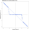 |
Fig. 8 Graphical representation of the interval-based error function computed on simulated data, for a fixed ground truth of 10. The plot shows the 10%-width error function with a transition zone of 20% of the half width of the error-interval. The blue dashed line indicates the residuals and the grey vertical dotted lines indicate the transition zones. |
 |
Fig. 9 Schematic of a three-fold CV process. The original training data are divided into three non-overlapping subsets. Each fold is held out in turn while models are fitted to the remaining training folds. Performance metrics, such as MSE or R2, are estimated using the retained fold in a given iteration. The CV estimate of the model performance is given by the average of the three performance estimates. |
4 Experimental design
We applied XGBoost to build regressor models, each of which was trained using the hold-out method, where the data sets described in Sect. 2.2 were split into training and testing subsets, in an 80-to-20 percent ratio. This proportion was reflected in the following distribution: in the case of DS0, DS1, DS2, and DS7, the training and testing sets comprised 11 930 and 2983 instances, respectively; DS3 and DS5 consisted of 11484 observations in the training set and 2872 elements in the testing set; finally, for DS4 and DS6, 10 881 instances were for the training set and 2721 for the testing one. We converted all training and testing sets to XGB dense matrices for efficiency and speed, as recommended by the authors of the xgboost package (Chen & Guestrin 2016). During the training phase, we used a 10-fold CV with five repetitions, where the best values for the hyperparameters were sought using a search grid on the training set. In all cases, the testing sets remained unseen by the models until the prediction and model evaluation phase. That is, the instances belonging to the testing sets were at no time part of the model learning process, behaving as new, unknown observations, as it would happen in a real-life scenario.
The experiment was carried out in two iterations. In the first iteration, we searched for the best values of the hyperparameters using a two-step grid search: firstly, the best parameters were searched for within a set of possible values; the search was then refined on the learning rate and the sub-sample ratio of training instances, by varying the parameter in a finer grid centred on the best value found in the previous step. Typically, no more than 1500 iterations were run for each submodel, and we activated a stopping criterion, where the learning for a given model would stop if the performance did not improve for five rounds. The grid values for each parameter were as follows: (a) colsample_bytree: the fraction of columns to be randomly subsampled when constructing each tree; it was searched within the set {1/3, 1/2, 2/3}7. (b) eta, η: the learning rate, was first searched within the values {0.03, 0.04, 0.05, 0.06, 0.07, 0.08, 0.09, 0.1}; the search was then refined by looking for five values centred on the best η found in the first iteration, each 0.01 apart. (c) gamma, γ: the minimum loss reduction required to further partition a leaf node of the tree; it was chosen within the set of values {0,1, 3, 5, 10}. (d) max_depth: the maximum depth per tree; during the first iteration, the best value was chosen from the set of integers {5L, 6L, 7L}; in the subsequent iteration, the optimal value was selected from the set {7L, 8L, 9L}. (e) min_child_weight: the minimum sum of instance weights required in a child node, which in a regression task is simply the minimum number of instances needed in each node; this parameter was searched for within the grid of integers {1L, 5L, 10L, 20L}. (f) subsample: the subsample ratio of the training instances; we opted for both stochastic and regular boosting, and so during the first grid search, subsample was chosen within eleven possible values, between 0.5 and 1, varying in steps of 0.05; the best value of the parameter found in the first grid search was then refined by searching for the optimal of five values centred on this best value or, if the latter was 1, by searching for the best of three values less than 1, each 0.05 apart in all cases. We tried other XGB hyper-parameters, but we found that these had the greatest impact on the performance of the model. The grid produced a maximum of 12 672 + 25 submodels during training, not counting the 10-fold CV with five repetitions.
In the second iteration, we refined the grid search, by using three values per hyperparameter, centred on the optimum for each parameter found in the first iteration. The grid is given in Table 2. The rationale for iteration 2 was to search for two additional values for each hyperparameter around the optimal value found in iteration 1. In the case of eta and subsample, care was taken not to exceed the allowed limits for these hyperparameters. The training produced a maximum of 729 + 20 submodels, not counting the CV.
After being trained by performing a grid search on the selected hyperparameters, the models were evaluated, and the importance of each feature was assessed in terms of the predictive power of the model, using the variance of the responses. The following sections present results and analysis for all models obtained during both iterations.
Set of possible values used for the hyperparameter grid search in iteration 2.
Best set of values for the XGB hyperparameters after performing a grid search.
5 Results
In Table 3, we present the results of the parameter optimisation carried out in iterations 1 and 2. As far as the hyperparameters are concerned, we highlight the following points by comparing the results of Table 3 with the original grid of Sect. 4:
colsample_bytree: In iteration 1, the optimal value was 1/2 or less for all the remaining models except DS0; thus, in the data sets comprising less predictors, fewer variables were randomly subsampled. In iteration 2, the tendency to reduce the number of randomly sampled variables with smaller sets remained.
eta: In the first iteration, η remained below 0.05, with 0.02 being the most common value; so, smaller values were prioritised; this came at the cost of longer convergence times and the risk of over-fitting, so we relied on gamma for a more conservative approach. In iteration 2, the most common learning rate value was 0.02, and only in one situation was the best value 0.03.
gamma: In iteration 1, γ was equal to 5 or 10 in three models, imposing the most conservative constraint of the options offered – this happened for the lowest (0.02) optimal value of the learning rate; nevertheless, this lowest η value also correlated with the low γ value of 1 in four models; this suggests, as expected, that the optimal values for these hyperparameters are also dependent on the data set in question and the values of the other hyperparameters. In the second iteration, γ was observed to vary between 0 and 5, with 3 being the most common value; in DS5, no constraints were applied to the model, and in no case was the most conservative value of 10 imposed.
max_depth: In iteration 1, it was always equal to 7, which is the maximum value offered by the grid. Iteration 2 offered cases with higher values (8 and 9) and, except for the DS1, DS2, and DS4 models, 9 was the best value; it was never equal to 7.
min_child_weight: In the first iteration, the most common value was 20 and the minimum value was 10; therefore, highly regularised models were generated, with smaller trees than when this hyperparameter was equal to 1 (the default value) – this limited a possible perfect fit for some observations, but made the models less prone to overfitting and compensated for smaller values of η and γ. In the second iteration, similarly to the previous case, DS1, DS2, and DS3 were the models with the highest degree of regularisation; the most common values were 15 and 20, and with them the trend towards models with smaller trees.
subsample: It was equal or close to 1.0 (never below 0.90) in both iterations, and so regular boosting was prioritised, despite the range of values suitable for stochastic boosting available in the grid.
The models were built using the optimal sets of the hyperparameters found by the grid search, and the algorithm was stopped after nrounds iterations, as given in the last row of Table 3. We had set the maximum number of possible iterations during the learning phase to 1500. In the case of DS2 in iteration 2, the stopping criterion was not activated, so we extended the maximum rounds to 2000 and found an optimal hyperparameters for nrounds equal to 1516.
The performance of the models obtained by applying XGB to the aforementioned data sets for predicting stellar rotation periods is summarised in Table 4. The number of predictors used to train the models is given under each data set in the header of the table. The quantities used to assess the quality of the models were described in Sect. 3.3.
Overall, the XGBoost models were wrong, on average, approximately between 4.1 and 9.0% of the time in iteration 1, and between 4.1 and 8.5% of the time in iteration 2, as indicated by µerr. DS4 was the least likely to make an error, and DS5 had the best adjusted R-squared.
Excluding DS0, the 10%-accuracy varied between 85.4 and 89.6% in iteration 1, and between 86.1 and 89.7% in iteration 2, with an increase of about 2 to 4 points when stars with rotation periods shorter than 7 d and greater than 45 d were removed and the number of predictors was reduced to the 28 most important. In the case of DS7, there is also an increase compared to DS1 and DS2. However, it is less significant than in the other cases. Therefore, the 10%-accuracy seems to increase with smaller data sets and especially with an improvement in data quality. The evolution of the interval-based accuracy with the error tolerance for the models obtained during iteration 2 is illustrated in Fig. 10. Overall, DS0 stands out from the other models, and the interval-based accuracy increases with the error tolerance, that is, when we are willing to accept larger errors. We find that (i) upon the exclusion of DS0, it is possible to identify two distinct groups of models: the first, composed of DS1, DS2, and DS7, with lower accuracies; and the second, containing the remaining models, with higher interval-based accuracies; (ii) particularly within the lowest error tolerance regime, there is a discernible enhancement in the accuracies of DS2 over DS1 and DS7 over DS2, i.e. when we run an initial selection of variables, as described in Sect. 2.2, and reduce the set of predictors to the most relevant ones; (iii) overall, DS1 is the model with the worst accuracy; (iv) in the highest tolerance regime, DS4 reaches values that are comparable to those of DS0; (v) DS7 consistently outperforms DS1 and DS2; (vi) there is a noticeable increase in performance when potentially problematic targets, i.e.stars with rotation periods above 45 d and below 7 d, are removed, especially for lower error tolerances; and (vii) the performance increases further when only the 28 most important predictors are used to train the models, with the interval-based accuracy always remaining above 87%.
The adjusted-R2 measured on the testing set was always equal to or greater than 94%. The model with the best goodness of fit measured by this metric was DS3 with 96%, followed by DS5 with 95%. These values seem to indicate a slightly greater ability of the predictors to explain the variability of the response when stars with short rotation periods (less than 7 d) are kept in the data set used to train the model. When compared with the corresponding unadjusted coefficients of determination, these  values were all of the same magnitude within each model, with differences typically to the third decimal place.
Figure 11 shows the RMSE and MAE differences between the testing and training sets – ∆RMSE (blue thick line) and ∆MAE (red thin line), respectively – and the difference between the two, ∆RMSE – ∆MAE (dotdashed grey line), for all the models generated in iteration 2. It can be observed that both differences, ∆RMSE and ∆MAE, reach a minimum value with DS0; following an initial increase in DS1 and DS2, a tendency towards a decrease can be identified as the data sets get smaller and the quality of the data increases. However, even if the downward trend continues, these differences reach values greater than the previous models in the case of DS2 and DS68. The general downward trend in the solid lines indicates that, with the exception of DS6, the degree of overfitting is less pronounced with the number of the model, i.e. with data sets comprising a smaller number but more relevant predictors and higher data quality. In iteration 2, ∆RMSE varied between 1.55 d for DS0 and 2.26 d for DS2. The latter was, therefore, the model with the highest degree of overfitting. After DS0, DS5 was the model with the least over-fitting. The highest degree of overfitting occurred for DS2. A similar behaviour was also observed in the case of∆MAE, where it reached the minimum value of 0.48 d for DS0 and a maximum of 0.93 d for DS2. The difference ∆RMSE – ∆MAE suggests that, with the exception of DS2 and DS6, the variance of individual errors generally decreased with smaller data sets. This greater overfitting did not prevent the models from performing slightly better in iteration 2 than in iteration 1. We can also see that the overfitting is less pronounced in DS7 than in DS2 and is similar to DS1. The evolution of these differences is in line with the behaviour of the adjusted R2, and seems to indicate that the removal of rotation periods shorter than 7 d and larger than 45 d has a positive impact on the performance of the models.
The mean values of the standard deviations for each model,  , and the ratio between these uncertainties and the mean values of the predictions carried out on the testing set,
  , estimated in uniform bins of unit length centred on integer values, are indicated in Table 5. For each prediction, the associated error bar is taken to be equal to the standard deviation in the corresponding bin. The values are indicative of the variability of the predictions. The mean length of the error bars oscillates between 0.28 and 0. 29 d, while the mean relative uncertainty is approximately equalto 1.2%, ranging between 0.0115 and0.0122. Furthermore, two additional rows have been included in this table, which indicate the proportion of under- and overestimates for all the models. It can be observed that the models exhibit a slight tendency to underestimate the predictions, as can be seen for DS1, DS2, DS3, DS5, and DS7.
The scatter plots of the ground truth against the predicted values for all the models built during iteration 2 are shown in Fig. 12 and, with additional marginal density plots, in Fig. A.3. The blue dashed lines indicate the identity function, and the red solid lines represent the linear models between the predicted and actual values. In order to enhance the clarity of the plot, the error bars associated with the predictions have been omitted. Most of the points fall on or near the y = x line, but some outliers can be seen, representing both under- and over-predicted cases. Nevertheless, all graphs show a high degree of positive correlation between the predicted and the reference values of the stellar rotation periods, indicating that there is generally good agreement between the predictions and the ground truth. This is confirmed by the marginal histograms and density plots for both the predicted and reference values in each panel of Fig. A.3, which are similar in terms of centrality, dispersion, and kurtosis. The dispersion of the observations relative to the identity line is not significantly large in all the models, but it increases with the predictions, namely, it has different values for low and high values of the response, which is an indication of heteroscedasticity. Moreover, the dispersion around the identity function is not exactly symmetric in all cases. For DS2 and DS7, we observe a change from predominant overestimates to underestimates around 25 d, while for models DS3 to DS6, this pattern occurs for rotation periods around 30 d. However, all models exhibit similar behaviour around y = x. The prevalence of overestimates and underestimates below and above a certain rotation period is approximately balanced on average. The R-squared reported in the panels correspond to the coefficient of determination between the predicted and the reference values. As expected, they are not significantly different from the  reported in Table 4, given the large total number of observations, n. The F-statistics shown in the graphs result from testing the null hypothesis that all of the regression coefficients are equal to zero. Overall, the F-tests and the corresponding p-values considered in the panels indicate that the sets of independent variables are jointly significant. Models DS0, DS1, DS2, and DS7 exhibit a similar performance for rotation periods shorter than about 50 d. If we consider rotation periods longer than 50 d, the dispersion is lowest for DS7.
In Fig. 13, we plot the ratio between the predicted and the reference values (top panel), and the ratio between the ground truth and the predictions (bottom panel), both against the reference values. The former highlights the over-predictions, while the latter emphasises the under-predictions. The highest over-and under-prediction ratios are equal to 44.4 and 30.2, respectively. There are nine under-prediction ratios equal to infinity, corresponding to zero values predicted by the model (we made negative predictions equal to zero). The largest ratios occur only for predictions close to zero, i.e. for very small rotation periods, typically below 7 d, corresponding to fast rotators. It can be seen that above the 7 d threshold, both the overestimations and the underestimations are at most about four times the reference values.
The Tukey-Anscombe (TA) plots of the raw residuals and of the 10%-error are shown in Fig. 14. For each model, the y-axis in the top panel corresponds to the residuals calculated on the rotation periods (in days), and in the bottom panel to the interval-based error calculated on the rotation frequencies (in days−1). The x-coordinate always represents the predictions in days. In all the plots, the points fluctuate randomly around the horizontal line passing through zero, forming a cloud that is approximately symmetrical around it. However, this cloud is not rectangular in shape. A detail of the TA plot for DS0, where we have constrained the y-axis to vary between −2 and 2, is shown in Fig. 15. We have added a regression line to the graph, which does not show a meaningful slope. The variance of the residuals increases with the predictions, indicating some degree of heteroscedasticity. All models share this characteristic of the TA plot.
The most important predictors for the models obtained in iteration 2 are highlighted in the bar plots of Fig. 16. Apart from DS0, the variables belonging to the CS and GWPS families typically contributed the most to the models. In the case of DS0 (the only data set where they were present), the rotation periods were naturally the dominant variables. Having obtained DS1, DS2, DS3 and DS4, we calculated the union of the 20 most important variables for these models. We were left with a set of 28 predictors, which we used to create the DS5, DS6, and DS7 data sets and their respective models. These variables are indicated in Table 6. The predictors that contributed most to the models are shown on the y-axis of Fig. 16. For models DS0 to DS4, we show the 30 most relevant variables for training; for the rest of the models, the plots show the 28 most important predictors mentioned above. We emphasise that the ‘Astro’ variables, such as the mass and the effective temperature, although they had some relevance for DS0, DS1, and DS2, they contribute little to the DS3 and DS4 models. TS-type variables, such as the photometric activity proxy, have some relevance and are important to support the model – we observe a drop in model performance when they are removed.
Quality assessment of the XGBoost models generated during iterations 1 and 2.
 |
Fig. 10 Evolution of the interval-based accuracies with the error tolerance. Models are indicated in different colours. The lines correspond to a locally weighted scatterplot smoothing (LOESS) regression of the accuracies for each model. The 10%-accuracy is highlighted by the vertical gray-shaded column in the background. The model with the highest overall accuracy was DS6. |
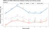 |
Fig. 11 RMSE and MAE differences, respectively: the ∆RMSE (blue thick line) and ∆MAE (red thin line), between the testing and training sets for the models generated in iteration 2. For both the RMSE and MAE, the differences are highest at DS2 and lowest at DS0. The dot-dashed grey line indicates ∆RMSE – ∆MAE, which is maximum at DS2 and minimum at DS4 and DS5. |
Mean error bars, in days (first row), ratio between the uncertainty and the average predicted values (second row), and the proportion of under- (third row) and over-estimates (last row) for each model.
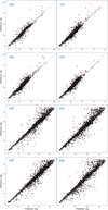 |
Fig. 12 Scatter plots of the reference rotation period as a function of the predicted values for the models built in iteration 2. The blue dashed lines indicate the identity function and the red solid lines represent the linear model between the ground truth and the predictions. DS7 has been placed next to DS1 and DS2 to facilitate model comparisons. |
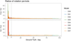 |
Fig. 13 Predictions over the ground truth (top panel) and its inverse (bottom panel) for the models obtained in iteration 2. The top plot highlights the magnitude of over-predictions, while the bottom plot highlights the amplitude of under-predictions. |
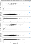 |
Fig. 14 Tukey-Anscombe plots (i) of the crude residuals computed on the rotation periods (top panels) and (ii) of the 10%-error computed on the rotation frequencies (bottom panels) for the models constructed during iteration 2 (continues on the next column). |
6 Discussion
The main findings from this work are highlighted in Figs. 10, 12, and 16. On the basis of the latter, if DS0 is excluded, the results show that the three most important variables for predicting rotation periods of K and M stars from the Kepler catalogue arguably belong to the Composite Spectrum and the Global Wavelet Power Spectrum groups, and specifically are cs_gauss_3_1_20, cs_gauss_3_1_55, and gwps_gauss_3_1_55. After removing features containing rotation period values from the data set, these variables were always in the top ten in terms of importance and stood out from the rest of the features. They correspond to the standard deviation of the first Gaussian fitted to the CS and GWPS for the 20-and 55-day filters, respectively. Not only these three predictors, but most of the CS and GWPS features with a non-negligible positive or negative correlation with the response are relevant to the predictive performance of the models. In addition, other variables, such as gwps_gauss_2_2_20, cs_gauss_2_2_20, gwps_gauss_2_2_55, cs_gauss_2_2_55, f_07, sph, h_cs_20, teff, and length have some relevance to the training of the models. In the specific case of the central periods of the second Gaussian function fitted in the GWPS and CS, although they are not the most relevant variables when training the models, the degree of importance assigned by the XGBoost algorithm to them can be attributed to the fact that the ground truth values were extracted from the central periods of the first fitted Gaussian functions, in conjunction with the algorithm’s inherent ability to identify harmonic sequences. The 20 and 55-day filters are more relevant than the 80-day ones, given that K and M stars typically exhibit relatively slow rotation periods and the filter at 80-day may potentially be susceptible to instrumental issues.
For the most important predictors, we used tree-based approaches to build our models, which by their nature do not suffer from the inclusion of highly correlated features. However, interpretability tools, such as importance estimations like the plots of Fig. 16, are hampered by collinearity and multicollinearity. If two features are perfectly correlated, such as cs_gauss_3_1_20 and cs_gauss_1_1_20, they are likely to be selected by the algorithm. In boosting, a link between a predictor and the response will remain stable once it has been learned by the model and so, the algorithm will stick to one of the correlated variables (but not both). This can be seen for the pair of correlated variables above and others, such as cs_gauss_1_1_20 and cs_gauss_1_1_55 or sph_cs_err_80, or gwps_gauss_2_2_55 and gwps_gauss_3_3_20 (just to name a few). We end up realising that one of the variables plays an important role in generating predictions, but we do not realise that the other variable is also important in the link between the observations and the response unless we perform a correlation analysis of the features (Chen et al. 2018), as we did in Sect. 2.3. In this sense, any of the features identified as most important, in particular the CS and GWPS variables based on the standard deviation of the fitted Gaussian, could in principle be replaced by any other predictor highly correlated with them without significant loss of model performance. In addition, as can be seen in the panels of Fig. 16, the GB importance profile typically has a steep slope because the trees from boosting are interdependent and thus present correlated structures as the gradient evolves. As a result, several predictors are selected across the trees, increasing their importance.
We believe that the level of importance attained by the CS and GWPS families of variables is related to the fact that most of the reference stellar rotation periods have been estimated from them. As mentioned in Sect. 2.3, there is a strong correlation between some features of these families and the response. One way to test this hypothesis would be to train new models from structured data obtained from synthetic light curves, produced by reliable stellar simulators, such as the StarSim code (Rosich et al. 2020) or the PLATO Simulator (Marcos-Arenal et al. 2014)9. This might require the engineering of new variables, but in principle we would be able to control for the correlations between the predictors and the response.
The results indicate that the CS features are slightly more important for the model than those of the GWPS. This is probably due to the fact that the CS is the product of the normalised GWPS and the ACF, thus amplifying peaks present in both and attenuating signals possibly due to instrumental effects, that manifest themselves differently in the GWPS and the ACF.
The most important TS variables are the activity proxies. They are relevant in the sense that they are often in the top ten of the most important variables. It then becomes apparent that it is important to extract all possible activity proxies (photometric, magnetic, and others) directly from the light curves and to use them as predictors when building a model.
The weakest features for predicting stellar rotation periods are the astrophysical ones. They are rarely included in the top ten most important variables. The exceptions are the mass and the effective temperature, which sometimes make it into the top 30 and were somewhat relevant to train DS0, despite the use of rotation periods as explanatory variables. This is consistent with the fact that it is not possible to predict stellar rotation periods from astrophysical variables alone. However, the FliPer metrics are strongly correlated with some of the CS and GWPS predictors, as shown in Sect. 2.3. Therefore, it is expected that the FliPer metric, which is a proxy for the total power spectral density of a star, can play an important role in a regression ML model based on GB. This means that the FliPer metrics could in principle replace any of the CS or GWPS features with which they are strongly correlated without significant loss of performance of the model. The parameter space may also play a role in the small contribution of the Astro predictors. We cannot exclude the possibility that examining a wider parameter space might change the picture, although we usually find a correlation in a narrower parameter space and not in a wider one.
In selecting the most important predictors common to all data sets from DS1 to DS4, it is possible that some variables relevant to DS5 and DS6 may have been overlooked. An example is the mass, which was not selected for the final set of independent variables because it was not within the top 20 most important predictors for DS3 and DS4. Therefore, perhaps a more prudent approach, analogous to the methodology employed to generate DS2, should be used when identifying the most relevant predictors.
As seen in Fig. 10, DS0 naturally stands out from the other models because it includes rotation periods in its explanatory variables. This fact is also responsible for the considerable discrepancy in the number of iterations required to achieve the optimal model observed between the training of DS0 and that of the remaining models. Reducing the number of predictors favours the XGB models, especially for lower error tolerance regimes, as can be seen from the fact that DS7 performs better overall than DS0, DS1 and DS2, as well as the enhanced performance in terms of interval-based accuracy of DS3, DS4, DS5, and DS6 in comparison to all other models10. In particular, DS7 is on average less wrong, and has comparable accuracy, testing RMSE and MAE, and adjusted R2 to the other models. If anything, it has the same tendency to overfit, and has less variance than DS0, DS1 and DS2 for slower rotators. However, the selection of predictors must be made with great care to prevent eliminating variables that are important for training the model. Our approach of selecting the 20 most important variables common to the initial four models might have been less optimal, given the lack of significant performance improvement observed in DS6 relative to DS4.
The differences between the training and testing RMSE and MAE (although natural) indicate a degree of overfitting during the training process of the models built from the DS0 to DS7 data sets. They vary between the models generated with the different data sets, indicating dissimilar levels of variation of the individual errors. However, these differences are not significant, even in the case of DS2, where they reached the highest value – this seems to be related to the initial selection of predictors.
Prior to rotation period filtering, the models struggled to predict some of the very short rotation periods, typically less than a few days, and periods greater than 45 d. These discrepancies are evident in the scatter plots of the models trained on the DS0 to DS6 data sets, and are further highlighted in Fig. 13. The over-and under-predictions are larger for very short rotation periods, below 7 d. Therefore, cases corresponding to K and M stars with rotation periods below 7 d or above 45 d are not suitable for training a predictive model using Kepler data. This is mainly due to the fact that (a) Kepler’s quarters are 90 days long, (b) at least two full cycles are required to obtain reliable observations, (c) the process of stitching two or more Kepler time series is not trivial and error-free, and (d) signals from stars with rotation periods of less than 7 d can be mimicked by fluxes from close binaries, classical pulsators, and other sources of confusion. After the filtering of the rotation periods, the predictive power of the XGB models improved, as shown by the analysis of the models learned from DS3 to DS6. By restricting the predictors to the set of the 28 most important variables identified by the XGB models built with DS0 to DS4, and by filtering in stars with rotation periods between 7 and 45 d, we were able to train computationally cheap but solid models, with good predictive performance.
While the final models are characterised by a goodness of fit around 96 %, there are still a few outliers with predictions varying from approximately from 50 to 200% of the actual values. The dispersion around the identity function is not exactly symmetric in most cases. This may be indicative of a limitation inherent to the models, whereby shorter periods are slightly overestimated and longer periods are slightly underestimated. However, it is probable that the dearth of data pertaining to rotation periods exceeding the 30 d and falling below the 20 d threshold is a significant contributing factor to this observed asymmetry. Moreover, it is likely that the error bars underestimate the overall uncertainty resulting from differential rotation when compared to the solar case and other K and M stars (Balona & Abedigamba 2016; Küker et al. 2019). In principle, increasing the number of training cases, controlling the errors in the measurements, and (most importantly) having a uniform distribution of training rotation periods (only possible with simulated data) would help to circumvent this problem and to improve the predictive power of the models. Furthermore, we could perform feature engineering on the original light curves to try to get a better set of predictors.
Finally, our results are in line with those of Breton et al. (2021). Taking into account the rotation periods in the explanatory variables, if we focus on the 10% interval-accuracy metric, the classifier created with B21 achieved comparable results. However, we have to take into account the fact that our accuracy metric is an approximation to the counterpart used to assess the quality of a classification model. In addition, we did not visually check the results, nor did we change them after testing the model. An important aspect to highlight is the fact that we used the ‘hold-out method’, namely, we used an unseen-before testing set to assess the quality of the model. This testing set was not part of the training of the model, nor did it participate in the CV performed to optimise the hyperparameters of the models. When assessing the quality of a model on a testing set, the predictive performance is typically more pessimistic than that obtained during the training with CV (Hastie et al. 2009; Torgo 2011). The accuracies claimed by Breton et al. (2021) appear to be obtained with a process that is similar to a 2-fold CV with 100 repetitions, performed on the whole data set. Therefore, even considering that their method is protected by the fact that they use the values of the target variable as predictors, we would expect the performance of their classifier to decrease slightly if the quality of the model were assessed on an unseen-before testing set.
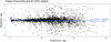 |
Fig. 15 Detail of the Tukey-Anscombe plot for DS0 during iteration 2, where we have restricted the y-axis to the values −2 and 2. The plot shows no meaningful slope, but it is possible to identify some degree of heteroscedasticity. |
Most important predictors obtained in iteration 2.
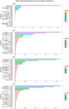 |
Fig. 16 Variable importance for the best models generated in iteration 2. In all models except DS0, the most important predictor was cs_gauss_2_1_55, followed by gwps_gauss_2_1_55 (continues on the next column). |
7 Conclusions
In this paper, we present a novel method based on a machine learning approach to calculate the stellar rotation periods for thousands of stars. We employed a regression analysis that makes use of tabular data extracted from light curves and that is based on the XGBoost algorithm. Recently, attempts have been made to apply ANN to light curves and classification RFs to tabular data to make such predictions. On the one hand, the former typically requires high computational resources; on the other hand, with respect to the latter, we argue that: (a) a classifier may not be the best approach to predict the rotation period because it is a continuous variable and (b) using rotation periods as predictors may weaken the predictive performance of the model in the presence of unseen testing data, which do not contain rotation period values and have not been used to train the model.
Our main objective was to build robust and efficient ML models for automatically predicting stellar rotation periods of K and M stars from the Kepler catalogue. To this end, we applied the regression XGBoost algorithm to train models from seven data sets built from the data originally published by Santos et al. (2019) and Breton et al. (2021).
Given that Breton et al. (2021) built a classifier with their data set (B21), we developed an interval-based error and a metric, the interval-based accuracy, which allowed us to convert predicted rotation periods into a proportion of successful events. We used this metric as a way to directly compare the results obtained with the two approaches (regression versus classification).
Initially, we used all the stars available in the base training set, namely, no stars were filtered out of the data set for model training. Overall, the results show that the predictive performance of the models trained on DS0, a data set equivalent to B21, is comparable to the performance of the classifier trained on the latter – if we keep rotation periods as independent variables and are willing to accept a 10% error in the predictions. If we remove the rotation periods from the predictors, we get a 10%-accuracy of about 90%. The goodness of fit, as measured by the mean absolute value of the relative residuals, µerr, and by the adjusted coefficient of determination,  , indicates that our models are robust, able to explain most of the variability in the response (approximately 96%), and are on average wrong no more than 8% of the time.
When we filter out stars with rotation periods below 7 d and above 45 d, the overall performance of the models increases, with about 94% to 96% of the variability of the response explained by the predictors, and the 10% interval-accuracy equal to about 96%. In this case, the models were on average wrong about 4% to 6% of the time.
The mean relative uncertainty, as indicated by the extent of the error bars, was estimated to be approximately 1.2% for all the models. There is also an increase in the quality of the XGB models when the number of predictors is reduced through the selection of the most important variables that contribute to the learning process.
In view of the results reported in Sect. 5, we conclude that the variables belonging to the CS and GWPS families are the most important for training a reliable XGBoost model with good predictive performance. TS-type features, namely, those related to the structure of the light curve, such as Sph, also have some relevance with respect to estimating stellar rotation periods. Although Astro-type variables, corresponding to astronomical observables and derived variables, do not have a significant weight in the importance plots, the FliPer metric and hence the power spectral density of a star can play a relevant role in model training, as they are strongly correlated with some of the variables in the CS and GWPS families.
By selecting the most important features, as measured during the training of the models obtained with the data sets DS0 to DS4, and excluding stars with rotation periods below 7 d and above 45 d, due to the characteristics of the Kepler space observatory and astrophysical constraints, we were able to build an optimal subset of predictors from the set of available explanatory variables, from which robust regression ML models with a good predictive performance could be trained. Our results clearly show that XGBoost models trained on these reduced size data sets have comparable or better performance than the models we previously obtained with the data sets DS1 to DS4. We claim a reduction of about 140 predictors when compared to the largest data set (DS0). The most important predictors, as measured by the xgboost R package, are the standard deviations of the first Gaussian functions fitted to the CS and GWPS, followed by the photometric index proxy, Sph. By using a data set consisting mainly of these variables, it is possible to train XGB models with a performance comparable to or better than those built on much larger data sets. By reducing the size of the sets by this order of magnitude, we are able to significantly improve the training time. With the resources we had available, namely, shared machines running multiple processes simultaneously, we were able to reduce the time to build a model by several hours.
In conclusion, the enhancement of data quality plays a pivotal role in the generation of accurate predictions using an XGBoost model. The reduction of the number of predictor variables while retaining the most important ones for model training represents a significant key contribution.
The current limitations of our methodology are primarily due to the lack of training of the models to deal with false positives. Given the numerous sources of confusion, including binaries, classical pulsators, red giants signals, and even misclassified stars, we intend to apply this methodology to simulated data. This will enable us to consider all the known factors that could result in false detections and to train the models to address them.
Acknowledgements
Nuno R. C. Gomes acknowledges support from the Atlantic Fisheries Fund research grant AFF-NS-1544 (Canada) and the “Science and technology for the Ariel mission: Contribution of the IEEC” project PID2021-125627OB-C31/MICIN/AEI/10.13039/501100011033/FEDER, of the European Union (Spain). Fabio Del Sordo acknowledges support from a Marie Curie Action of the European Union (Grant agreement 101030103) and “María de Maeztu” award to the Institut de Ciències de l’Espai (CEX2020-001058-M). We would like to express our gratitude to the reviewer for their perceptive comments and recommendations, which have contributed to the enhancement of the quality of this manuscript. We gratefully acknowledge the CINECA award under the ISCRA initiative for the availability of high-performance computing resources and support, Sergio Messina and Nuccio Lanza for useful discussions, and Eva Ntormousi for comments on the manuscript. Nuno Gomes and Fabio Del Sordo would like to pay tribute to Luís Torgo, who left us far too soon.
Appendix A Plots
In this appendix, we present a number of additional graphs to complement the information presented in the main body of the paper. All figures were previously referenced, except those relating to elapsed times.
Figure A.1 shows the correlations between predictors belonging to the Astro and CS families of variables, and the response. Variables that are highly correlated with each other, such as sph_cs_20 and f_07, can in principle be swapped in the model without loss of performance. The situation is similar for the predictors belonging to the GWPS family of variables, whose correlations are shown in Fig. A.2. Only negative or weak correlations with the response are shown in these plots. However, features that are strongly correlated with the target variable would be highlighted in full plots of the CS and GWPS predictors and the target variable.
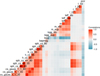 |
Fig. A.1 Correlations between the Astro variables, some of the CS predictors, and the response. The F0.7 and F7 FliPer metrics are highly correlated with some CS variables. |
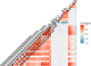 |
Fig. A.2 Correlations between the Astro variables, some of the GWPS predictors, and the response. Similarly to Fig. A.1, the F0.7 and F7 FliPer metrics are highly correlated with some GWPS variables. |
Figure A.3 shows the scatter plots of the ground truth versus the predictions for the models generated during iteration 2, including the marginal density plots of the predictions and the reference rotation periods. Similar to Fig. 12, the blue dashed line indicates the identity function. Each panel reports the goodness of fit and significance of the relationship, using R2, the F-test and the corresponding p-value, respectively. Overall, the sets of predictors are jointly significant.
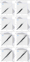 |
Fig. A.3 Scatter and marginal density plots of the reference rotation period as a function of the predicted values for the models built during iteration 2. The blue dashed lines indicate the identity function. DS7 has been placed next to DS1 and DS2 to facilitate comparison of the models. |
The total learning time per model in iterations 1 and 2 is shown in Fig. A.4. In order to optimise the generation of the models, the hyperparameter grids were divided into several sub-grids (12 and nine in iteration 1 and 2, respectively), which were started in parallel. In this way, the longest models, with more than 150 h of learning time, took less than 24 h to complete, as shown in Fig. A.5. Using this approach, the fastest models in iteration 2 took less than two hours to train.
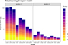 |
Fig. A.4 Total learning time per model in iterations 1 and 2. To build the models, the hyperparameter grids were split into 12 and nine sub-grids in iteration 1 and 2, respectively. The height of the scripts is proportional to the amount of time it takes to execute them. |
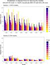 |
Fig. A.5 Breakdown of learning times for the models in iteration 1 and 2. Even though the total run time amounted to 150 h in iteration 1 (see Fig. A.4), the longest models took no more than 24 h to complete. |
References
- Aerts, C., Mathis, S., & Rogers, T. 2019, ARA&A, 57, 35 [Google Scholar]
- Angus, R., Beane, A., Price-Whelan, A. M., et al. 2020, AJ, 160, 90 [Google Scholar]
- Balona, L. A., & Abedigamba, O. P. 2016, MNRAS, 461, 497 [NASA ADS] [CrossRef] [Google Scholar]
- Barnes, S. A. 2003, ApJ, 586, 464 [Google Scholar]
- Baron, M. 2019, Probability and Statistics for Computer Scientists (Chapman and Hall/CRC) [CrossRef] [Google Scholar]
- Bicz, K., Falewicz, R., Pietras, M., Siarkowski, M., & Pres, P. 2022, ApJ, 935, 102 [NASA ADS] [CrossRef] [Google Scholar]
- Biehl, M., Bunte, K., Longo, G., & Rino, P. 2018, in ESANN, European Symposium on Artificial Neural Networks, Computational Intelligence and Machine Learning, ed. M. Verleysen, vol. 26 (Ciaco - i6doc.com), 307 [Google Scholar]
- Bonanno, A., & Corsaro, E. 2022, ApJ, 939, L26 [NASA ADS] [CrossRef] [Google Scholar]
- Blancato, K., Ness, M. K., Huber, D., Lu, Y. L., & Angus, R. 2022, ApJ, 933, 241 [NASA ADS] [CrossRef] [Google Scholar]
- Borucki, W., Koch, D., Batalha, N., et al. 2009, in Transiting Planets, 253, 289 [NASA ADS] [Google Scholar]
- Borucki, W. J., Koch, D., Basri, G., et al. 2010, Science, 327, 977 [Google Scholar]
- Bouvier, J., & Bertout, C. 1989, A&A, 211, 99 [NASA ADS] [Google Scholar]
- Breiman, L. 2001, Mach. LEARN., 45, 5 [NASA ADS] [CrossRef] [Google Scholar]
- Breton, S. N., Santos, A. R., Bugnet, L., et al. 2021, A&A, 647, A125 [NASA ADS] [CrossRef] [EDP Sciences] [Google Scholar]
- Brown, T. M., Latham, D. W., Everett, M. E., & Esquerdo, G. A. 2011, AJ, 142, 112 [Google Scholar]
- Brun, A. S., & Browning, M. K. 2017, Living Rev. Solar Phys., 14, 1 [NASA ADS] [CrossRef] [Google Scholar]
- Bugnet, L., García, R., Davies, G., et al. 2018, A&A, 620, A38 [NASA ADS] [CrossRef] [EDP Sciences] [Google Scholar]
- Cantiello, M., & Braithwaite, J. 2011, A&A, 534, A140 [NASA ADS] [CrossRef] [EDP Sciences] [Google Scholar]
- Chen, T., & Guestrin, C. 2016, XGBoost: A Scalable Tree Boosting System [Google Scholar]
- Chen, T., Benesty, M., & He, T. 2018, Understand Your Dataset with Xgboost, https:cran.r-project.org/web/packages/xgboost/vignettes/discoverYourData.html, Accessed on 2022-09-18 [Google Scholar]
- Claytor, Z. R., van Saders, J. L., Llama, J., et al. 2022, ApJ, 927, 219 [NASA ADS] [CrossRef] [Google Scholar]
- Claytor, Z. R., Van Saders, J. L., Cao, L., et al. 2024, ApJ, 962, 47 [NASA ADS] [CrossRef] [Google Scholar]
- Damasso, M., Del Sordo, F., Anglada-Escudé, G., et al. 2020, Sci. Adv., 6, eaax7467 [CrossRef] [Google Scholar]
- Eggenberger, P., Miglio, A., Montalban, J., et al. 2009, Effects of rotation on the evolution and asteroseismic properties of red giants [Google Scholar]
- Friedman, J. H. 2001, Ann. Statist., 1189 [Google Scholar]
- García, R., Ceillier, T., Salabert, D., et al. 2014, A&A, 572, A34 [NASA ADS] [CrossRef] [EDP Sciences] [Google Scholar]
- Géron, A. 2017, Hands-on machine learning with Scikit-Learn and TensorFlow: concepts, tools, and techniques to build intelligent systems (O’Reilly Media, Inc.) [Google Scholar]
- Hall, O. J., Davies, G. R., van Saders, J., et al. 2021, Nat. Astron., 5, 707 [NASA ADS] [CrossRef] [Google Scholar]
- Hastie, T., Tibshirani, R., & Friedman, J. 2009, The Elements of Statistical Learning: Data Mining, Inference, and Prediction, 2nd edn. (Springer) [Google Scholar]
- Haykin, S. 2009, Neural Networks and Leraning Machines (PHI Learning), 944 [Google Scholar]
- Howell, S. B., Sobeck, C., Haas, M., et al. 2014, PASP, 126, 398 [Google Scholar]
- Huber, D., Bryson, S. T., Haas, M. R., et al. 2016, The K2 Ecliptic Plane Input Catalog (EPIC) and Stellar Classifications of 138,600 Targets in Campaigns 1-8 [Google Scholar]
- Hyndman, R. J., & Koehler, A. B. 2006, Int. J. Forecast., 22, 679 [CrossRef] [Google Scholar]
- James, G., Witten, D., Hastie, T., & Tibshirani, R. 2013, Springer Texts in Statistics, 103, An Introduction to Statistical Learning - with Applications in R (New York: Springer) [CrossRef] [Google Scholar]
- Kuhn, M., Johnson, K., et al. 2013, Applied Predictive Modeling, 26 (Springer) [CrossRef] [Google Scholar]
- Küker, M., Rüdiger, G., Olah, K., & Strassmeier, K. G. 2019, A&A, 622, A40 [NASA ADS] [CrossRef] [EDP Sciences] [Google Scholar]
- Lu, Y., Angus, R., Agüeros, M. A., et al. 2020, AJ, 160, 168 [Google Scholar]
- Marcos-Arenal, P., Zima, W., De Ridder, J., et al. 2014, A&A, 566, A92 [NASA ADS] [CrossRef] [EDP Sciences] [Google Scholar]
- Mathur, S., Huber, D., Batalha, N. M., et al. 2017, ApJS, 229, 18 [Google Scholar]
- McQuillan, A., Mazeh, T., & Aigrain, S. 2014, ApJS, 211, 24 [Google Scholar]
- Messina, S. 2021, A&A, 645, A144 [NASA ADS] [CrossRef] [EDP Sciences] [Google Scholar]
- Messina, S., Nardiello, D., Desidera, S., et al. 2022, A&A, 657, L3 [NASA ADS] [CrossRef] [EDP Sciences] [Google Scholar]
- Mullally, S. 2020, MAST Kepler Archive Manual [Google Scholar]
- Murphy, K. 2012, Machine Learning: A Probabilistic Perspective, Adaptive Computation and Machine Learning (MIT Press) [Google Scholar]
- Pichara Baksai, K. E., Protopapas, P., & Leon, D. 2016, ApJ, 819, 18 [NASA ADS] [CrossRef] [Google Scholar]
- Pontius, R. G., Thontteh, O., & Chen, H. 2008, Environ. Ecol. Statist., 15, 111 [NASA ADS] [CrossRef] [Google Scholar]
- R Core Team 2023, R: A Language and Environment for Statistical Computing (Vienna, Austria: R Foundation for Statistical Computing) [Google Scholar]
- Ramachandran, K. M., & Tsokos, C. P. 2020, Mathematical Statistics with Applications in R (Academic Press) [Google Scholar]
- Raschka, S., & Mirjalili, V. 2017, Python Machine Learning, 2nd edn. (Livery Place 35 Livery Street Birmingham B3 2PB, UK: Packt Publishing Ltd.) [Google Scholar]
- Ricker, G. R., Winn, J. N., Vanderspek, R., et al. 2014, SPIE Conf. Ser., 9143, 914320 [Google Scholar]
- Rosich, A., Herrero, E., Mallonn, M., et al. 2020, A&A, 641, A82 [NASA ADS] [CrossRef] [EDP Sciences] [Google Scholar]
- Santos, A. R. G., García, R. A., Mathur, S., et al. 2019, Surface rotation and photometric activity for Kepler targets I. M and K main-sequence stars [Google Scholar]
- Santos, A., Breton, S., Mathur, S., & García, R. 2021, ApJS, 255, 17 [NASA ADS] [CrossRef] [Google Scholar]
- Skumanich, A. 1972, ApJ, 171, 565 [Google Scholar]
- Strassmeier, K. G. 2009, A&AR, 17, 251 [CrossRef] [Google Scholar]
- Torgo, L. 2011, Data Mining with R: Learning with Case Studies (Chapman and Hall/CRC) [CrossRef] [Google Scholar]
- Van Saders, J. L., Ceillier, T., Metcalfe, T. S., et al. 2016, Nature, 529, 181 [NASA ADS] [CrossRef] [Google Scholar]
The R programming language (R Core Team 2023) was used for all code and data analyses.
Words in brackets, in typewriter font, refer to variable names as they appear in Table 1 and in the data frames.
In Breton et al. (2021), Sph is divided into several values, each corresponding to the process from which it was obtained (ACF, CS, or GWPS) and to the filter applied to the light curves (20, 55, or 80 days).
The KEPSEISMIC time series are available from the Mikulski Archive for Space Telescopes (MAST), via the link https://dx.doi.org/10.17090/t9-mrpw-gc07
Note that while ϵ∆,δ depends on δ, acc∆ does not.
Two other hyperparameters belonging to this family of subsam-pling columns were initially optimised: colsample_bylevel and colsample_bynode. However, no improvement in model performance was observed when they were included, and as they work cumulatively, only colsample_bytree was retained in the optimisation process in the end.
There is a marginal increase in ∆MAE in DS4 compared to DS3.
PLATO stands for PLAnetary Transits and Oscillations of the stars.
We ran several tests, where we removed the features labelled “prot_”, but kept the central periods of the first Gaussian functions fitted to the CS and GWPS; we found that, in these cases, DS7 outperformed DS0. In fact, when the rotation period information was retained in the predictors, each of DS5, DS6, and DS7 performed better than DS0.
All Tables
Names of the 170 predictors, as they appear in the original data set, and their description.
Mean error bars, in days (first row), ratio between the uncertainty and the average predicted values (second row), and the proportion of under- (third row) and over-estimates (last row) for each model.
All Figures
|
Fig. 1 Histograms (left panels) and box-plots (right panels) of the target variable, prot, on DS0 (top row) and on the training set generated from it (bottom row). The distributions are very similar to each other, right skewed, with medians equal to 23.87 d, minima and maxima of 0.53 d and 98.83 d, respectively. Both have several outliers. |
| In the text | |
|
Fig. 2 Similar to Fig. 1, but for the DS4 data set. The distributions are very similar to each other, approximately symmetrical, with means of 24.44 d and 24.43 d, and standard deviations of 9.11 d and 9.07 d, on DS4 and its training set, respectively. |
| In the text | |
|
Fig. 3 Histogram (left panel), box-plot (middle panel), and QQ-plot (right panel) of the rotation period errors, |
| In the text | |
|
Fig. 4 Rotation period errors, |
| In the text | |
|
Fig. 5 Correlations between the Prot variables and the response. In this case, all predictors are highly correlated with the target variable. |
| In the text | |
|
Fig. 6 Correlations between the TS variables and the response. |
| In the text | |
|
Fig. 7 Correlations between the ‘Astro’ variables and the response. |
| In the text | |
|
Fig. 8 Graphical representation of the interval-based error function computed on simulated data, for a fixed ground truth of 10. The plot shows the 10%-width error function with a transition zone of 20% of the half width of the error-interval. The blue dashed line indicates the residuals and the grey vertical dotted lines indicate the transition zones. |
| In the text | |
|
Fig. 9 Schematic of a three-fold CV process. The original training data are divided into three non-overlapping subsets. Each fold is held out in turn while models are fitted to the remaining training folds. Performance metrics, such as MSE or R2, are estimated using the retained fold in a given iteration. The CV estimate of the model performance is given by the average of the three performance estimates. |
| In the text | |
|
Fig. 10 Evolution of the interval-based accuracies with the error tolerance. Models are indicated in different colours. The lines correspond to a locally weighted scatterplot smoothing (LOESS) regression of the accuracies for each model. The 10%-accuracy is highlighted by the vertical gray-shaded column in the background. The model with the highest overall accuracy was DS6. |
| In the text | |
|
Fig. 11 RMSE and MAE differences, respectively: the ∆RMSE (blue thick line) and ∆MAE (red thin line), between the testing and training sets for the models generated in iteration 2. For both the RMSE and MAE, the differences are highest at DS2 and lowest at DS0. The dot-dashed grey line indicates ∆RMSE – ∆MAE, which is maximum at DS2 and minimum at DS4 and DS5. |
| In the text | |
|
Fig. 12 Scatter plots of the reference rotation period as a function of the predicted values for the models built in iteration 2. The blue dashed lines indicate the identity function and the red solid lines represent the linear model between the ground truth and the predictions. DS7 has been placed next to DS1 and DS2 to facilitate model comparisons. |
| In the text | |
|
Fig. 13 Predictions over the ground truth (top panel) and its inverse (bottom panel) for the models obtained in iteration 2. The top plot highlights the magnitude of over-predictions, while the bottom plot highlights the amplitude of under-predictions. |
| In the text | |
|
Fig. 14 Tukey-Anscombe plots (i) of the crude residuals computed on the rotation periods (top panels) and (ii) of the 10%-error computed on the rotation frequencies (bottom panels) for the models constructed during iteration 2 (continues on the next column). |
| In the text | |
|
Fig. 15 Detail of the Tukey-Anscombe plot for DS0 during iteration 2, where we have restricted the y-axis to the values −2 and 2. The plot shows no meaningful slope, but it is possible to identify some degree of heteroscedasticity. |
| In the text | |
|
Fig. 16 Variable importance for the best models generated in iteration 2. In all models except DS0, the most important predictor was cs_gauss_2_1_55, followed by gwps_gauss_2_1_55 (continues on the next column). |
| In the text | |
|
Fig. A.1 Correlations between the Astro variables, some of the CS predictors, and the response. The F0.7 and F7 FliPer metrics are highly correlated with some CS variables. |
| In the text | |
|
Fig. A.2 Correlations between the Astro variables, some of the GWPS predictors, and the response. Similarly to Fig. A.1, the F0.7 and F7 FliPer metrics are highly correlated with some GWPS variables. |
| In the text | |
|
Fig. A.3 Scatter and marginal density plots of the reference rotation period as a function of the predicted values for the models built during iteration 2. The blue dashed lines indicate the identity function. DS7 has been placed next to DS1 and DS2 to facilitate comparison of the models. |
| In the text | |
|
Fig. A.4 Total learning time per model in iterations 1 and 2. To build the models, the hyperparameter grids were split into 12 and nine sub-grids in iteration 1 and 2, respectively. The height of the scripts is proportional to the amount of time it takes to execute them. |
| In the text | |
|
Fig. A.5 Breakdown of learning times for the models in iteration 1 and 2. Even though the total run time amounted to 150 h in iteration 1 (see Fig. A.4), the longest models took no more than 24 h to complete. |
| In the text | |
Current usage metrics show cumulative count of Article Views (full-text article views including HTML views, PDF and ePub downloads, according to the available data) and Abstracts Views on Vision4Press platform.
Data correspond to usage on the plateform after 2015. The current usage metrics is available 48-96 hours after online publication and is updated daily on week days.
Initial download of the metrics may take a while.