| Issue |
A&A
Volume 689, September 2024
|
|
|---|---|---|
| Article Number | A114 | |
| Number of page(s) | 22 | |
| Section | Planets and planetary systems | |
| DOI | https://doi.org/10.1051/0004-6361/202450429 | |
| Published online | 06 September 2024 | |
Modeling the Enceladus dust plume based on in situ measurements performed with the Cassini Cosmic Dust Analyzer
1
Space Physics and Astronomy Research Unit, University of Oulu,
Finland
e-mail: vveyzaa@gmail.com
2
Institut für Geologische Wissenschaften, Freie Universität Berlin,
Germany
e-mail: juergen.schmidt@fu-berlin.de
3
Universität Stuttgart, Institut für Raumfahrtsysteme,
Stuttgart,
Germany
4
Laboratory for Atmospheric and Space Physics, University of Colorado,
Boulder,
USA
5
Los Alamos National Laboratory,
Los Alamos,
USA
Received:
18
April
2024
Accepted:
3
July
2024
We analyzed data recorded by the Cosmic Dust Analyzer on board the Cassini spacecraft during Enceladus dust plume traversals. Our focus was on profiles of relative abundances of grains of different compositional types derived from mass spectra recorded with the Dust Analyzer subsystem during the Cassini flybys E5 and E17. The E5 profile, corresponding to a steep and fast traversal of the plume, has already been analyzed. In this paper, we included a second profile from the E17 flyby involving a nearly horizontal traversal of the south polar terrain at a significantly lower velocity. Additionally, we incorporated dust detection rates from the High Rate Detector subsystem during flybys E7 and E21. We derived grain size ranges in the different observational data sets and used these data to constrain parameters for a new dust plume model. This model was constructed using a mathematical description of dust ejection implemented in the software package DUDI. Further constraints included published velocities of gas ejection, positions of gas and dust jets, and the mass production rate of the plume. Our model employs two different types of sources: diffuse sources of dust ejected with a lower velocity and jets with a faster and more colimated emission. From our model, we derived dust mass production rates for different compositional grain types, amounting to at least 28 kg s−1. Previously, salt-rich dust was believed to dominate the plume mass based on E5 data alone. The E17 profile shows a dominance of organic-enriched grains over the south polar terrain, a region not well constrained by E5 data. By including both E5 and E17 profiles, we find the salt-rich dust contribution to be at most 1% by mass. This revision also results from an improved understanding of grain masses of various compositional types that implies smaller sizes for salt-rich grains. Our new model can predict grain numbers and masses for future mission detectors during plume traversals.
Key words: astrobiology / astrochemistry / planets and satellites: composition / planets and satellites: fundamental parameters
© The Authors 2024
 Open Access article, published by EDP Sciences, under the terms of the Creative Commons Attribution License (https://creativecommons.org/licenses/by/4.0), which permits unrestricted use, distribution, and reproduction in any medium, provided the original work is properly cited.
This article is published in open access under the Subscribe to Open model. Subscribe to A&A to support open access publication.
1 Introduction
Since the discovery of Saturn’s E ring (Feibelman 1967; Smith et al. 1975), the bright icy moon Enceladus was suspected to be the source of the dust that forms this ring because its orbit is located within the densest part of the ring (Showalter et al. 1991). Cryo-volcanic activity at Enceladus, as a source of the dust, was one of the suggested explanations for the E ring origin (Pang et al. 1984; Haff et al. 1983; Showalter et al. 1991; Kargel & Pozio 1996). This hypothesis was confirmed by the Cassini space mission, which discovered an active region around Ence-ladus’ south pole and a plume of gas and dust emitted from there (Dougherty et al. 2006; Spencer et al. 2006; Porco et al. 2006; Hansen et al. 2006; Spahn et al. 2006; Dougherty et al. 2018).
The south polar terrain (SPT) of Enceladus is a geologically young region with a diverse relief abounding with fractures and giant boulders (Spencer et al. 2006; Porco et al. 2006; Martens et al. 2015). The most prominent features of the region are four fissures of more than 100 km in length and up to 2 km in width. The so-called tiger stripes (TSs) are named Alexandria, Cairo, Baghdad, and Damascus. The composition of the materials ejected with the plume (Postberg et al. 2009, 2011; Postberg et al. 2018b, 2023; Hsu et al. 2015; Waite et al. 2017; Khawaja et al. 2019) gives strong evidence that the fissures tap a subsurface ocean of likely global extension (Thomas et al. 2016) with a crust thickness below 5 km around the south pole (Le Gall et al. 2017). The details of the connection (Spencer et al. 2018), the formation history of the cracks (Hemingway et al. 2020), and their role in the heat budget and activity cycle (Kite & Rubin 2016; Berne et al. 2023) are the subjects of ongoing research.
In the fissures that are connected to the ocean, one expects to find a table of liquid water at a depth that is given by the hydrostatic pressure balance and modulated by tidal flexing of the ice (Kite & Rubin 2016). The conditions near the water surface must be close to the triple point of water because ice, liquid water, and water vapor coexist there. A backpressure will develop in the fissure when the gas flows through narrow cracks to the surface (Schmidt et al. 2008). The flux of the gas carries icy dust grains, forming the plume.
The SPT of the moon is also notable for an anomalous output of heat. According to the observed IR brightness, the estimates for the power emitted from SPT lie between 5.8 ± 3.1 GW and 15.8 ± 3.1 GW (Spencer et al. 2006; Howett et al. 2011). A significant contribution from the terrain between the TSs is possible (Spencer et al. 2018; Howett et al. 2022).
Between 2005 and 2015, Cassini performed 23 close flybys of Enceladus with multiple instruments observing the moon, the E ring, and the plume (see Table 1). Observations in various ranges of wavelengths, radar measurements, and in situ sampling of gas and dust allowed researchers to develop a modern vision of the Enceladus plume (for a review see e.g. Postberg et al. 2018a).
In this work we mostly focus on data collected in situ with the Cassini Cosmic Dust Analyzer (CDA) (Srama et al. 2004) in the Enceladus plume. The CDA consisted of two subsystems: the High Rate Detector (HRD) and the Dust Analyzer (DA). The HRD was a dust counter capable of registering impacts of dust grains to its sensors with a rate of up to 104 s−1. The DA had as one of its subsystems the Chemical Analyzer (CA) that was a mass spectrometer capable of analyzing the dust grains’ composition. Owing to the time necessary to process the signal, the CA was saturated by counts above a certain rate (Kempf 2008), which was always the case inside the plume or in the E ring’s densest parts. The CA generally observed smaller particles than the HRD, though for both instruments the range of detectable grain sizes depended on the spacecraft velocity. Postberg et al. (2011) modeled the variations of the proportion of salt-rich dust particles in the first compositional profile that was obtained for the Enceladus dust plume recorded during the E5 flyby in 2008. Since then, more compositional profiles of the Enceladus dust plume were obtained, as well as a number density profiles recorded by HRD. In this work, we construct a new dust plume model that is constrained by all CDA data sets available from plume traversals. These profiles are those obtained by the HRD during the E7 and E21 flybys as well as the profiles from the E5 and E17 flybys obtained by the CA. An additional compositional profile was obtained at flyby E18, but it is of insufficient quality and therefore not suited for fitting the model.
The dust grains from the Enceladus plume consist mostly of water ice. In addition to water ions, spectral lines of simple organic compounds were found in the mass spectra recorded by the CA in the E ring and in the plume (Postberg et al. 2008). A smaller fraction of particles contains sodium and potassium salts (Postberg et al. 2009) with a salinity at the level of 1%. The latter particles suggest the presence of liquid water under the surface of the moon because in this abundance, salts cannot condense on a dust grain from a gaseous phase (see Sect. 3 in Supplementary material of Postberg et al. 2009). A fraction of the spectra recorded by the CDA contains complex organics (Postberg et al. 2018b; Khawaja et al. 2019), which when combined with the presence of liquid water, sparks interest in Enceladus from an astrobiological point of view (McKay 2020; Hand et al. 2020).
The paper is organized as follows. In Sect. 2, we discuss the available data sets and recent advances in the interpretation of the difference between salt-poor grains with and without organ-ics as well as an updated derivation of the size range of the grains whose spectra were recorded by the CA. Then in Sect. 3, we summarize the previous analysis of the compositional profile from E5. In Sect. 4, we describe our new model, the choice of dust sources on the SPT, and the distribution functions for the grain ejection and size. We detail the application of the model to the CDA data and derive and motivate suitable choices for the parameters. Sect. 5 presents the main results as well as a comparison of the profiles of number density and abundance of various compositional types obtained from the model. Sect. 6 provides a summary of our work and a discussion of the results.
Parameters specific to the CDA and geometric parameters for the Enceladus flybys considered in this paper.
2 Cosmic Dust Analyzer in situ data from the plume
In this section we present the data collected by the Cassini CDA inside the plume during five flybys of Enceladus, covering a time span of 7 years. Four flybys (E5, E7, E17, E21) yielded plume profiles of good quality, and the E18 profile was noisy (Table 1). The flyby geometries are shown schematically in Fig. 1 and the projected spacecraft ground tracks on the SPT in Fig. 2. The measurements during each flyby represent a one-dimensional cut through the plume, providing either a profile of number density from HRD (E7 and E21) or a compositional profile from DA (E5, E17). HRD recorded grain number density profiles for different mass thresholds simultaneously. We also derive here the range of grain sizes to which the measurements were sensitive, depending on the spacecraft velocity relative to Enceladus during the flyby under consideration.
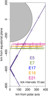 |
Fig. 1 Trajectories of the Cassini flybys at Enceladus studied in this paper. The thick line denotes the part of the E5 trajectory where Cassini was passing through the densest part of the plume and the CDA instrument was saturated and no meaningful data was obtained. The E17 line is hidden under the E18 line. |
2.1 Main compositional types and relation to grain size
Before we turn to the compositional profiles we briefly review the main compositional types that were inferred from the CA mass spectra recorded in the E ring and in the Enceladus plume (Postberg et al. 2009). Table 2 summarizes the main compositional types of dust in the Enceladus plume. Type I spectra show mostly water ions and traces of salts at a very low mixing ratio. Type II spectra additionally contain organics. These are in most cases simple volatile organic compounds (Khawaja et al. 2019), while 3% bear also complex and refractory, macromolec-ular organics (Type II HMOC, HMOC for High Mass Organic Cations, Postberg et al. 2018b). Type I and Type II, with a proportion of salts in the range 10−8−l0−5 (Postberg et al. 2009), are also referred to as the salt-poor particles.
In contrast, type III particles are salt-rich with a salinity of about 1%. Therefore, these salt-rich grains instead appear to be derived from salty oceanic spray at the liquid water interface beneath Enceladus’s surface. In the uppermost part of the ocean, exsolved gases (CO2), and potentially water that boils in the low-pressure environment, form bubbles that rise to the interface of the liquid and the gaseous phase. From bubbles bursting at this interface, a spray is produced from the ocean water (Postberg et al. 2009, 2011; Porco et al. 2017; Postberg et al. 2018b). The small salty droplets are carried upward by the gas flux, freeze, and serve as the cores for condensation of water vapor from the gas. It is likely that volatile organic compounds entrained in the vapor flow will likewise condense onto salty type III ice grains when they rise upward through the icy vents (Khawaja et al. 2019). However, the high salinity can substantially reduce CDA’s sensitivity for trace organic compounds (Napoleoni et al. 2023a,b) and currently organic compounds have not been identified in published CDA data of type III grains.
The CDA mass spectra are derived from the temporal evolution of the charge recorded by the multiplier (MP) of CDA after a grain has hit the Chemical Analyzer Target of the instrument (Srama et al. 2004). The total charge collected on the ion grid for a given impact is called the QI charge (given in Coulombs). The QI charge is a fraction of the positive total charge contained in the plasma produced in the impact (the impact charge yield) that depends on the impact speed, the mass, and the composition of the grain. It can be estimated from an empirical fit to CDA calibration data
![$m[{\rm{kg}}] = \left\{ {\matrix{ {77771.0{{\left( {{{QI} \over \upsilon }} \right)}^{1.31}},\upsilon < {\upsilon _{{\rm{th}}}},} \cr {48.2{{\left( {{{QI} \over {{\upsilon ^5}}}} \right)}^{0.91}},\upsilon > {\upsilon _{{\rm{th}}}},} \cr } } \right.$](/articles/aa/full_html/2024/09/aa50429-24/aa50429-24-eq1.png) (1)
(1)
where v is given in kilometers per second and m in kilograms. Here
![${\upsilon _{{\rm{th}}}}\left[ {{\rm{km}}\,\,{{\rm{s}}^{ - 1}}} \right] = {\left( {{{48.2} \over {77771.0Q{I^{0.4}}}}} \right)^{{{1.0} \over {3.25}}}}$](/articles/aa/full_html/2024/09/aa50429-24/aa50429-24-eq2.png)
is a QI dependent threshold velocity. This formula generalizes the empirical fit to lab data obtained by Srama (2000) that used a constant threshold velocity of 10 km s−1 throughout, potentially leading to unphysical jumps in the mass versus velocity relation for given QI.
The CDA only recorded useful spectra for charges roughly 2fC < QI < 2pC. For smaller QI charges, an impact does not produce a sufficient number of ions to record a mass spectrum of useful quality. Similarly, for larger QI charges the spectra become distorted, and their classification is impossible. These limiting QI values are constant and depend on the design of the CDA instrument only. Therefore, Eq. (1) allowed us (for given relative velocity of instrument and dust grain) to specify the range of grain masses for which spectra can be obtained. Upon assumption of a grain density this can be translated into a range of grain sizes to which the CA is sensitive.
The QI charge of an impact does not depend solely on the grain mass and impact velocity. There is also a material dependence expected. Namely, Timmermann (1989) conducted impact experiments with metal particles and compared the charge yields obtained when using metal targets and ice targets, respectively. Impacts on ice targets were found to produce fewer ions, which may suggest that the charge yield of an icy particle hitting a metal target may be lower as well. The Eq. (1) was obtained from analysis the iron particles impact on a metal target and thus, Eq. (1) may underestimate for given QI the mass (size) of the dust grain recorded by CA. At the same time, salts present in the icy grains are easy to ionize, increasing the impact charge yield, which makes the type III particles detectable even if they are small (Wiederschein et al. 2015). Consequently, the detectable size range of the CA for the salt-rich dust will be shifted toward smaller radii relative to the size range of the observed salt-poor particles. For this reason, when calculating sizes of the dust particles, we apply a correction to Eq. (1) assuming that the impact charge yield from an icy grain impact on CDA is 10 times lower in case of a salt-poor grain and 2.5 times lower (Wiederschein et al. 2015) in case of a salt-rich grain than the one predicted by Eq. (1). This effect is taken into account in the ranges of grain sizes given in Table 1 for the flybys E5 and E17. No significantly increased charge yield due to the addition of organics in water was observed in analog experiments (Nölle 2022). Therefore, our assumption to use an identical ion yield for both salt-poor types (Type I and II) grains is justified. We note that the use of Eq. (1) together with the correction factors for the particle material eventually leads us here to a different interpretation of the detected particle size than previous work on the CA mass spectra (Postberg et al. 2009, 2011).
By grain size we mean the equivalent radius of a particle with the inferred mass, assuming that the grain is spherical and has a homogeneous density of 920 kg m−3. It is important to keep in mind that the actually measured quantity is the charge entering the multiplier (QI), while the masses and the radii inferred from the QI charge are a subject to (potentially considerable) uncertainties. Finally, we note that there exist alternative calibration formulae for the QI signal inferred from independent lab experiments (Srama 2009), which adds to the uncertainty of any work that links CDA mass spectra to grain size.
For any given spacecraft speed the observed ion yield of type II grains is systematically higher than for type I grains. Judging from the aforementioned analog experiments (Nölle 2022) this cannot be attributed to a change in composition from organic compounds. Recently it was suggested by Khawaja et al. (2019) that the salt-poor types I and II represent in fact one compositional species and the non-occurrence of organics in type I is an instrumental effect that appears for small and/or slow grains. For a mass spectrum to have an ample signal-to-noise ratio to detect organic features, the charge yield of the impact must be sufficiently large. The charge yield depends on spacecraft velocity and particle size. Thus, for a given impact speed smaller particles with organic compounds in similar abundances produce fewer ions so that the organic compounds may not be visible in the mass spectrum. These are then considered to be type I spectra. Thus, it is suggested that the types I and II are representatives of the same dust population but type I is smaller than type II. From Eq. (1) it is clear that the threshold between type I and type II spectra will depend on the speed of the impact onto the instrument and hence on the relative velocity of the spacecraft and the dust particles. In other words, the relative abundance of type I and type II spectra is expected to depend on the flyby speed. This effect must be considered when interpreting and comparing the compositional profiles obtained in the plume from flybys with different relative speed.
As mentioned previously, there are two distinct subtypes of type II grains: Those exhibiting volatile organics of low molecular mass (Khawaja et al. 2019) and those with large quantities of refractory complex organics with much higher molecular masses (Postberg et al. 2018b). In contrast to the much more abundant subtype with low mass organics that are formed in an identical process to type I (homogeneous nucleation from the gas phase), the rare subtype with high mass organics cannot have formed this way and is instead suggested to from by heterogeneous nucleation around a solid organic condensation core (Postberg et al. 2018a,b; Khawaja et al. 2019). This latter rare case of salt-poor grains is excluded from our simulation at the current stage because of the sparsity of available data. Due to a restriction in its mass range CDA was insensitive to high mass organics during E5 and only one such particle was detected in the plume during E17, (Postberg et al. 2018b).
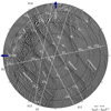 |
Fig. 2 Ground tracks of the Cassini flybys over the SPT of Enceladus. E5, E17, and E18 (shown in red) are flybys for which compositional spectra were obtained. From flybys E7 and E21 (shown in black), we used profiles of particle count rates to constrain our model. Cross symbols mark times measured from the respective closest approach of the spacecraft to Enceladus. |
Main compositional types of particles emitted from Enceladus.
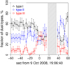 |
Fig. 3 Compositional profile recorded by the CDA during the E5 Cassini flyby at Enceladus. |
2.2 Cosmic Dust Analyzer compositional profiles of the Enceladus plume
Compositional profiles were obtained by the CDA during three close flybys at Enceladus labeled E5, E17, and E18. The profiles of the E5 and E17 flybys are shown in Figs. 3 and 4. These profiles may exhibit minor differences compared to previously published versions (Postberg et al. 2011; Postberg et al. 2018a) due to a revised analysis of the mass spectra contained in the data set.
For the E18 flyby, a large fraction of the spectra are noisy and could not be classified, so that these data do not provide additional information usable as a model constraint. The most probable explanation for the noisiness of the E18 compositional profile is an overloading of the CA with a high number of relatively large ice grains. This is consistent with E18 traversing the SPT close to Baghdad, which is one of the most active regions on Enceladus (Spitale & Porco 2007; Porco et al. 2014; Hedman et al. 2018).
During the E5 flyby, CDA was operating in a mode that allowed it to record mass spectra at a rate of five spectra per second, achieving a high temporal resolution and good statistics for the observational data set. Every data point in Fig. 3 represents the average fraction of the respective compositional type in a nine second time window (box car average, overlapping with the window of neighboring points). The grayed-out region in Fig. 3 between 18 and 35 seconds after closest approach to Enceladus corresponds to the passage of Cassini through the very dense central part of the plume (compare also to Fig. 1). The large number of dust impacts in this range seriously affected the instrument performance so that a reliable interpretation of the data was not possible.
During the E17 flyby, CDA recorded spectra at a lower rate. Data points in Fig. 4 also represent a box car average, but the averaging is performed over an interval of 60 s. The data points in Fig. 4 are not equidistant because the time of the data point is the mean of the spectra’s detection times in the bin. This is different from the central time of the bin. Although the E17 temporal resolution is five times lower than for E5, the spatial resolution is only two times lower due to the lower spacecraft velocity. Nevertheless, the E17 data are scarce and detailed features of the compositional profile may depend to some degree on the adopted binning. Therefore, we restricted our analysis on the main trends, as the increases in type II and type III proportions around closest approach, which are robustly visible for any choice of the binning.
There is a large difference in the flyby geometry of the E5 and E17 flybys. While E5 was encountering Enceladus on a steep trajectory with the closest approach at relatively low southern latitudes and a traversal of the plume at relatively high altitude, the E17 trajectory was equatorial, with the closest approach over the SPT at lower altitude (compare to Fig. 1 and Table 1). The passage of the SPT was perpendicular to the Tiger Stripes for E5, while it was parallel to the Tiger Stripes for E17 with a ground track between Cairo and Baghdad (Fig. 2). For the interpretation of the compositional profiles, the difference of the flyby speeds between E5 (17.7 km s−1) and E17 (7.5 km s−1) is important, because the speed of dust impacts onto the detector defines the detectable size range of the instrument (see Sect. 2.1). Thus, the spectra recorded by DA observed during the E5 and E17 flybys sample grains from a different part of the size distribution (see Table 1).
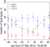 |
Fig. 4 Compositional profile recorded by the CDA during the E17 Cassini flyby at Enceladus. |
2.3 High Rate Detector profiles of the Enceladus plume
The HRD was a subsystem of Cassini CDA that counted dust particle impacts along the spacecraft trajectory with a rate up to 104 s−1 (Srama et al. 2004). The rate of detections along the spacecraft trajectory, γ(t), can be converted to the number density n of grains at the instantaneous spacecraft position from n = γ/A ⋅ vrel, where A is the product of the detector area and the CDA boresight vector and vrel is the relative velocity of the spacecraft and the dust configuration1,
HRD was composed of two polyvinylidene fluoride (PVDF) foil sensors mounted in front of the instrument with sensitive areas of 50 and 10 cm2, respectively. Each of these sensors had four counters, labelled M1,M2,M3,M4 for the larger foil and m′1,m′2,m′3,m′4 for the smaller foil. These counters correspond to threshold numbers of electrons at the input of the HRD charge amplifiers that depend on the mass and velocity of the impacting grain (Kempf et al. 2012) as
![${n_M} = 3.8 \times {10^{17}}{\left( {{m_d}[{\rm{g}}]} \right)^{1.3}}{\left( {{\upsilon _d}\left[ {{\rm{km}}\,{{\rm{s}}^{ - 1}}} \right]} \right)^{3.0}}$](/articles/aa/full_html/2024/09/aa50429-24/aa50429-24-eq3.png) (2)
(2)
for the larger (M) detector and
![${n_m} = 3.6 \times {10^{18}}{\left( {{m_d}[{\rm{g}}]} \right)^{1.3}}{\left( {{\upsilon _d}\left[ {{\rm{km}}\,{{\rm{s}}^{ - 1}}} \right]} \right)^{3.0}}$](/articles/aa/full_html/2024/09/aa50429-24/aa50429-24-eq4.png) (3)
(3)
for the smaller (m′) detector. Here, md and vd are the dust particle mass and impact velocity. The electron threshold numbers nM for the M1, M2, M3, M4 counters are 2.1 × 10⁶, 1.9 × 10⁷, 4.1 × 10⁸, 5.2 × 10⁹, and for the m′1, m′2, m′3, m′4 counters the threshold values of nm are 2.1 × 10⁷, 2.0 × 10⁸, 4.3 × 10⁹, 5.4 × 10¹⁰. This takes into account that during the E7 and E21 flybys the larger detector of the HRD was in “low-mass” sensitivity mode while the smaller detector was in “high-mass” sensitivity mode (for explanation on the sensitivity modes, see Srama et al. 2004; Kempf et al. 2012). The calibration of the reduced sensitivity mode (set for the smaller detector) is based on interpolation, and therefore, the thresholds for m′ counters are less reliable. We use prime notation to emphasize this difference in the two sensors’ data. All the counters are cumulative, that is, if M2 is triggered, then also M1 is triggered, and if M4 is triggered than also M1,M2, and M3 are triggered (and the same for the m′1, m′2, m′3, m′4 counters).
For a fixed spacecraft velocity, Eqs. (2) and (3) give the mass thresholds, and by assuming spherical grains with a density of 920 kg m−3, corresponding size thresholds are given for the flybys E7 and E21 in Table (1) for those counters that registered a sufficiently large number of grains, so that a profile could be derived. With rate profiles recorded in several counters, the HRD provides information about the size distribution of the local dust population.
We used as constraints for our model the number density profiles obtained by the HRD during the E7 and E21 Cassini flybys at Enceladus. Both correspond to nearly horizontal passages of the plume (Fig. 1) over the SPT at different altitudes. Their ground tracks are shown in Fig. 2. Each flyby yielded five profiles, corresponding to the counters M1, M2, M3 as well as m′1 and m′′2.The counters corresponding to larger size thresholds had not been triggered sufficiently often during the flybys so that number density profiles could not be derived. The profiles are shown in Figs. 5 and 6, where the zero of the horizontal axis corresponds to the moment of closest approach rounded to an integer second. The closest approach of the E7 flyby occurred in 2009 at altitude of 95 km above Enceladus’ south pole, and Cassini’s trajectory crossed all four Tiger Stripes. The recorded profiles show pronounced peaks corresponding to TS crossings (Fig. 5). During the E21 flyby in 2015 the spacecraft crossed only three TSs at a very low altitude above the SPT with the closest approach at 49 km above Enceladus’ surface. The density profiles are shown in Fig. 6. These profiles show a less detailed structure.
During the E5 flyby, the HRD recorded dust impacts but produced highly noisy data indicative of instrument overflow. This overflow could be attributed to an impact rate exceeding 105 s−1, pressure from the plume gas, or bombardment by nanograins, as the spacecraft traversed a dense part of the plume at high velocity. During the E17 flyby, the HRD-CDA system experienced a malfunction in its data transmission system, resulting in the failure to record a profile. Therefore, we lack simultaneous number density measurements to complement the available compositional profiles.
In some cases, we observe that two sensors expected to possess very similar size thresholds still yield noticeably different particle number densities (Figs. 5 and 6). During Cassini’s nominal tour, the match between the HRD m-sensor and M-sensor data was generally within 1 standard deviation (Kempf et al. 2008). However, during later mission phases, the differences grew larger, likely due to aging effects. The cratering of the foils reduces the sensitive area and decreases sensitivity to large particle impacts. If a new crater overlaps with an older crater, the resulting charge pulse is smaller, making the hit more likely to be attributed to a lower mass impactor. This is more likely to occur with larger impactors that create larger craters. Therefore, the higher mass channels are more strongly affected as seen in Figs. 5 and 6. The overall trend due to aging effects can be complex and is not necessarily linear or even monotonic because the aging of the instrument electronics due to the radiation exposure and general parts exhaustion may affect the data differently. The inconsistency in the two sensors’ observations provides an indication of the level of uncertainty in the inference of the size thresholds from the calibration formulae.
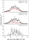 |
Fig. 5 Number density profiles of the E7 flyby recorded by HRD counters M1, m′1, M2, m′2, and M3. |
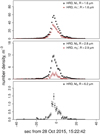 |
Fig. 6 Number density profiles of the E21 flyby recorded by HRD counters M1, m′1,M2, m′2, and M3. |
3 Previous model of the E5 compositional profile
In this section we briefly review our previous modeling of the E5 compositional profile (Postberg et al. 2011) and describe the necessity for its revision. In spite of the fact that dust is delivered to the E ring from the plume, the relative compositional abundances of the dust in the plume differ from the ones in the E ring. The first compositional profile of the Enceladus dust plume (Postberg et al. 2011) obtained during the E5 flyby (October 9, 2008) showed that the proportion of salt-rich dust becomes higher at the fringe of the Tiger Stripes. Postberg et al. (2011) explained this in terms of a correlation between grain size and compositional type. From a comparison of the distributions of the ion yields recorded by CDA for salt-poor and salt-rich particles in the E ring (see supplementary information of their paper) they concluded from the observation of larger ion yields of the salt-rich that grains of this type are, on the average, larger than the salt-poor. At the time of their analysis Postberg et al. (2011) did not take into account a potential material dependence of the ion yield (Timmermann 1989). Indeed, for not too large salt concentrations Wiederschein et al. (2015) found an increase of the ion yield with the concentration of salts in water droplets that we take into account in the current work (Sect. 2.1). In the Postberg et al. (2011) model, the larger salt-rich particles were ejected with smaller velocities, owing to the velocity slip when the grains are accelerated by the gas in the vents. The smaller salt-poor grains, in contrast, were ejected at higher speeds, much closer to the gas speed. The model of Postberg et al. (2011) was able to fit the compositional profile of the E5 flyby.
The compositional profile obtained from the E17 flyby (March 27, 2012), however, does not support this model. With a lower spacecraft velocity the CA observed larger grains at this flyby, so one would expect the proportion of salt-rich spectra to be even greater at E17 than at E5. But during the E17 flyby the increase in observed type III spectra near C/A to Enceladus remains small and the main feature of the E17 compositional profile is the pronounced increase in the proportion of salt-poor but organics-enriched type II spectra (Fig. 4). This cannot be reproduced within the model assumptions of Postberg et al. (2011). Thus, there is a need to revise the model. The very different flyby geometries (Figs. 1 and 2) as well as the drastically different impact speeds (and the corresponding observed size ranges) provide complementary data sets. These are optimal prerequisites for a comprehensive modeling approach.
4 New plume model and application to Cosmic Dust Analyzer data
In this section we describe our new model for the Enceladus dust plume that will be applied to the CDA data presented in Sects. 2.2 and 2.3. This new approach employs the two-body model for dust ejection by Ershova & Schmidt (2021) that relates the number density of dust in a given point in space with the dust dynamical properties at the moment when it was ejected from a point source on the surface of an atmosphereless body. This model is implemented as a software package DUDI2, which we utilized in our work. The whole Enceladus plume was then modeled by a large set of point sources placed on the SPT (details in Sect. 4.1). Our choice for the distribution of dust ejection velocities, the directional distribution of the ejection, as well as the dust size distribution for various compositional types are given in Sects. 4.2, 4.3, and 4.4, respectively. We also describe our method of taking into account the background of the E ring dust (Sect. 4.6) that adds to the measured signal and, therefore, is crucial for the fits to the data.
In view of the complexity of the problem at hand it is unavoidable that the model possesses a large number of parameters. These comprise, for instance, the settings for the distributions describing grain ejection and size. But already the choice for the functional form of these distributions offers a large amount of freedom. Also, we observed that some parameters have a similar quantitative effect on the model properties and there exist parameters that are not independent from each other, so that the effect of the change in one parameter can be compensated (approximately) by a variation of other parameters. For these reasons we refrained from applying a rigorous least squares method to estimate the parameters. Instead, we fixed certain parameters that are fundamental to the Enceladus plume from available observations like the positions of sources (Porco et al. 2014) or the gas ejection speed (Hansen et al. 2006; Tian et al. 2007; Smith et al. 2010; Dong et al. 2011). Then we modified and selected the remaining parameters manually (e.g., for the dust size distribution), within physically plausible limits. In this way we determined and reported properties of the Enceladus dust emission that our model must robustly possess in order to obtain a reasonably good fit to the CDA data.
4.1 Two types of dust sources
We implemented two types of sources, “jets” and “diffuse sources”, that differ in composition of ejected dust and in their mode of ejection. This was motivated, on one hand, by the observation of isolated jets (Hansen et al. 2008; Porco et al. 2014), that remain defined and stand out above the plume background to higher altitudes above the SPT. But, on the other hand, a more uniform background is observed as well in the dust distribution in high phase imaging of the plume (Spitale et al. 2015; Porco et al. 2015).
As the gas and dust flux in the vents ultimately derives from the underground water reservoir that has a salty spray above the water table, the salty type III particles are present in our model in both types of sources. The salt-poor dust is assumed to form by condensation from the vapor inside the channels.
Here, high levels of saturation, necessary for abundant condensation, are given in trans-sonic flow (Schmidt et al. 2008; Yeoh et al. 2015, 2017), allowing for gas acceleration above thermal velocity and leading to the existence of supersonic jets (Hansen et al. 2008; Portyankina et al. 2022). Therefore, in addition to salt-rich grains, jets in our model emit salt-poor type I and II particles, while the diffuse sources emit only type III dust. This leads to a dynamical differentiation of salt-rich and salt-poor dust, which is necessary to simultaneously reproduce the compositional profiles of E5 and E17.
For the jets, we adopted the list of 100 jets whose locations were inferred by Porco et al. (2014) from the analysis of high phase angle images. In our model, these jets are considered vertical, though we investigate the effect of their possible tilts in the Appendix (see Figs. A.1–A.3). More jets present on Baghdad and Damascus sulci making the plume denser in this region. It is supported by measurements of thermal emissions (Howett et al. 2011) and dust-to-gas ratio (Hedman et al. 2018). The overloading of the CA during the E18 flyby is also an indirect evidence of the higher activity on Baghdad. The diffuse sources in our model are distributed uniformly along all tiger stripes. Figure 7 shows the locations of all model sources.
In our model, we allowed for distributions of ejection speed and ejection angle (measured from the jet axis) that differ for the diffuse and jet sources. These are described in the following sections.
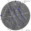 |
Fig. 7 Map of the SPT with the ground tracks of the Cassini flybys used to constrain our model. The locations of diffuse salt-rich sources and the jets from Porco et al. (2014) are shown as white and blue circles, respectively. |
4.2 Ejection speed distribution
One of the main features of our model is a grain-size dependent distribution of the particle speed at the moment of ejection. The expression for this distribution,
 (4)
(4)
was obtained by Schmidt et al. (2008) and was also used in previous work on the E5 compositional profile (Postberg et al. 2011) of the Enceladus plume (see also Sect. 3). This size-dependent velocity distribution explains the difference between the plume’s composition and the background composition of the E ring. Namely, when the dust is accelerated by the gas flux, smaller particles acquire higher velocities that allow them to rise to higher altitudes above the surface and have a greater probability to escape the moon’s gravity. Hence, more large particles are found closer to the sources. The properties of the velocity distribution (Eq. (4)) for particles of a given size R are regulated by two parameters: the speed of the gas flux ugas and the critical radius Rc.
There exist various estimates for the gas speed in the Enceladus plume (Hansen et al. 2006; Tian et al. 2007; Smith et al. 2010; Dong et al. 2011) ranging from thermal velocity (approximately 400 m s−1 for plausible conditions on Enceladus) to a several times higher value. The gas velocity likely varies across the SPT with maximal values exceeding 1000 ms−1 in the most active regions. In our modeling we used ugas = 400 m s−1 for all the diffuse sources and ugas = 800 m s−1 for all the jets (see Table 3).
In the distribution Eq. (4) the critical radius discriminates between small, fast grains, that are essentially ejected at gas velocity, and larger grains that are significantly decelerated relative to the gas (see Fig. 8). The relation of the critical radius to the parameters of the gas flow in the Enceladus vents was derived by Schmidt et al. (2008)
 (5)
(5)
where ρgas and ρdust are the mass densities of the gas and the dust grains, respectively. The square root term is the thermal velocity in the gas, with the gas temperature Tgas, the mass of a water molecule m0, and the Boltzmann constant kB. The quantity Lcoll is a typical length scale for the vents that sets the scale over which grains are accelerated by the gas flow. This may roughly correspond to the width of the vents themselves. Fitting their dust ejection model to the brightness stratification of the dust plume in images, Schmidt et al. (2008) constrained the value of Lcoll to the centimeter to decimeter range. In that case the value of Rc must be in the sub-micron range, which is consistent with modeling of VIMS data (Hedman et al. 2009). Generally, Rc cannot be too small because then it would be impossible for micron-sized particles to escape to the E ring, where they have been found. At the same time, it cannot be too big because otherwise the dust plume scale height would be larger than observed. Since the parameter Rc depends on gas density and velocity, and the width of the vents, it may have different values in different parts of the plume. When choosing parameters of the model, we assumed Rc = 0.05 µm for all diffuse sources and Rc = 0.2 µm for all jets (see Table 3). In this way we aimed to estimate the average value, though it is possible that the parameter Rc varies across the plume. The value of Rc that we applied for the jets in our model is close to the estimates of Hedman et al. (2009) and Postberg et al. (2011).
The parameters of the ejection speed distribution adopted in our model are listed in Table 3. We assumed that for diffuse sources Rc is generally smaller than for the jets, which establishes, in accordance with the role we ascribed to the diffuse sources in our model, a tighter confinement of the dust emitted from the diffuse sources closer to the surface. Physically, this could imply a smaller width (scale Lcoll) of the vents that supply the diffuse sources, perhaps consisting of a network of finer cracks in the close vicinity of the tiger stripes. But one may also speculate if a potentially turbulent gas flow affords a similar effect such that the size of turbulent vortices effectively plays the role of Lcoll, which is smaller than the actual width of the channels that feed the jets. Such effects may overcompensate the effect of the smaller gas speed (Eq. (5)) we adopted for diffuse sources, and thus, it is possible that Rc is in fact smaller for the diffuse sources than for the jets.
We chose the value for Rc of the diffuse sources based on the fits to the compositional profiles. A significantly larger Rc would cause a worse agreement with the E17 data. In such case the salt-rich dust within the size range observed during E17 would become too abundant before −20 s and after 20 s since the closest approach when Cassini was not flying directly above the SPT and the diffusely ejected salt-rich dust could potentially play a role. Using an Rc smaller than that of the jets for the diffuse sources allowed us to avoid this effect.
Parameters of the model dust sources.
4.3 Distribution of ejection directions
For the distribution of the polar angle ψ and azimuth λM of the particles’ ejection velocity vector, we employed
 (6)
(6)
This corresponds to a uniform distribution of the azimuth angle around the axis of ejection (expressed by the factor 1/2π) and a quasi-Gaussian distribution of the polar angle ψ. The value of the normalization constant Cnorm is determined numerically for given width ω of the Gaussian. Some of the images analyzed by Porco et al. (2014) show strongly confined jets that can be modeled with ω = 5° in Eq. (6). On the other hand, a wide jet can be understood as an ensemble of multiple narrow jets located close to each other and possessing a wide distribution of tilt angles. Here, we fixed the parameter ω by comparison to the HRD profiles (see Figs. A.4–A.7 in Appendix for details) and adopt for the ejection angle distribution Eq. (6) with ω = 10°. For the diffuse sources we set ω = 90°. We note, that these values of ω correspond for the distribution given by Eq. (6) to mean polar angles 〈ψ〉 of 12.5° and 54.3°, respectively.
We further investigate in the appendix the effect of non-vertical jets with inclinations to the normal as they were determined by Porco et al. (2014) (see Figs. A.1–A.3). For the fits of the CDA data to our models the difference between the cases of vertical and inclined jets is marginal. Furthermore, Southworth et al. (2019) found that strongly tilted jets would cause characteristic surface deposition patterns that are not seen in observational data. The absence of the deposition patterns tells us that highly tilted jets could be only short-lived features, so they may appear in images but cannot be active long enough to deposit a detectable amount of dust on the surface.
4.4 Size distribution
The number density profiles from HRD provide a better constraint on the size and ejection speed distribution in the jets, because dust from the jets dominates the space above the SPT. Moreover, the compositional profile of the horizontal E17 flyby (Fig. 4) suggests that the jets are in fact dominated by salt-poor dust. In turn, this means that the size distribution of salt-rich particles, and in general the ejection parameters of the diffuse sources, are not constrained so well by the HRD data.
The different processes that lead to the formation of the salt-rich and salt-poor particles, respectively, inspire the usage of a different functional form for their size distribution. Specifically, we used a power-law distribution,
 (7)
(7)
for the sizes of salt-poor grains that are believed to form via homogeneous nucleation inside the gas flow. In contrast, the salt-rich particles are believed to form from frozen droplets of water. It is natural to assume that their distribution has a peak because the droplet sizes themselves tend to have a peaked distribution (Spiel 1998). We adopted a log-normal distribution,
 (8)
(8)
for the size distribution of the salt-rich dust. The confinement of this distribution toward smaller grain size is necessary to obtain agreement with the E5 compositional profiles. A power law would produce a too large number of grains smaller than 0.2 µm. Accelerated by the gas to fairly high velocities, these would reach low southern latitudes sampled by the CDA before closest approach and result there in an over-abundance of salt-rich grains that is not seen in the data.
We truncated both distributions at small and at large grain sizes, so there are no particles smaller than 0.1 µm nor larger than 15 µm (‰ and Rmax in Eq. (7), respectively). The normalization constant Cnorm in Eq. (8) is not equal to  , as it would be in case of log-normal distribution; it is determined numerically. The value of the largest possible particle radius was chosen based on the largest size threshold of the HRD that was triggered in the plume. This corresponds to two impacts of grains >12.9 µm during the E7 flyby. The largest grains in the plume must be larger then this. We cannot constrain this limit very well; we come back to this point in the discussion in Sect. 5.3.
Figures 9 and 10 show the probability densities of the size distributions used in the model for the dust particles ejected from Enceladus. The respective size ranges are indicated where CDA could detect particles in the two flybys for salt-poor and salt-rich dust grains. In contrast to the assumptions of Postberg et al. (2009), our model now suggests that salt-poor type II grains are mostly larger than salt-rich grains of type III. This idea corresponds well with a recent systematic analysis of CDA distributions of the different compositional ice grain types in E ring (Nölle et al. 2024). This data set was taken mostly at similar impact speeds than at E17, suggesting that type 2 particles are mostly larger than type 3 grains in the E ring, too.
In order to model the compositional profiles of E5 and E 17, we needed to define a way to distinguish between type I and type II particles. The parametrization used for this purpose is based on the idea that the bigger a salt-poor particle is, the more chances it has to be identified as a type II because the larger ion yield enhance the chance to detect organic compounds in the spectrum (Postberg et al. 2018a; Khawaja et al. 2019, see also Sect. 2.1). The area under the curve for the size distribution of salt-poor grains (lower panels in Figs. 9 and 10 with size distribution Eq. (7)) within any given interval of particle radius equals the probability that the ejected salt-poor particle has a radius within that interval. The latter probability must now be divided between the two salt-poor types. To achieve this, we let the diagonal dashed blue line in Figs. 9 and 10 cut the area under the curve of the salt-poor size distribution. The area under the dashed blue line is equal to the probability of a type II particle to have a radius within the considered size bin and the area under the black line, but above the dashed blue line, is the probability of a type I grain’s radius to be within these limits. In this way, salt-poor particles up to a certain radius  are all considered to be type I; then the probability to be of type II rises linearly with the size increasing from
  to
to  ; finally, all salt-poor particles larger than
  are assumed to be of type II. The border between type I and type II is defined by the amount of ions produced in the impact that depends on the particle’s mass and on spacecraft velocity (higher ion yield from dust impact at higher speed). Therefore, the border is different for E5 and E17 flybys. The actual values of
  and
and  define the maximal fraction of type II spectra that can be obtained with the model. They were chosen to match the peaks in the proportion of type II in the two compositional profiles. The adopted values for
  and
and  are equal 0.2 and 0.4 µm for the E5 flyby, and 0.8 and 1 µm in case of E17. The diagonal line is defined as

Table 3 summarizes our parameters for the dust emitted by the jets and diffuse sources and their production rates in the model.
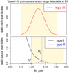 |
Fig. 9 Size distribution of freshly ejected salt-rich and salt-poor dust for E5 (at 17.7 km s−1). Yellow areas indicate the size ranges detectable by CDA. These are different for salt-rich and salt-poor dust. Radii |


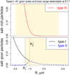 |
Fig. 10 Size distribution of freshly ejected salt-rich and salt-poor dust for E17 (at 7.5 km s−1). Yellow areas indicate the size ranges detectable by CDA. These are different for salt-rich and salt-poor dust. Radii |


4.5 Plume variability
Over the duration of the flybys the Enceladus plume activity can be considered constant, so each point source of the model is ascribed a constant production rate. However, there may be a difference between flybys. The plume shows a significant temporal variability (Hedman et al. 2013; Nimmo et al. 2014) on the scale of Enceladus’ orbital period around Saturn (which is also the moon’s diurnal period) and there is evidence for long-term variability over the years of Cassini’s observations (Ingersoll & Ewald 2017; Ingersoll et al. 2020). Inferring the relative production rate for the considered flybys from Fig. 8 of Ingersoll & Ewald (2017), we noted that while the E7 and E21 occurred at very different orbital phases, the overall activity level of the moon is expected to be similar. We can also evaluate the total production rate of the plume at the time of these two flybys using the HRD measurements. The E5 and E17 flybys occurred at a very similar position on Enceladus’ orbit around Saturn (see Table 1), which is close to the phase of maximal production rate over the diurnal cycle. At the same time, taking into account the additional long-term variability, the total dust production rate during the E17 flyby should have been lower.
Furthermore, the work of Sharma et al. (2023) provides evidence that the size distribution of dust grains in Enceladus’ plume varies over time. This may imply variations in the size or ejection speed distribution parameters. However, we assumed these parameters remain unchanged and varied only the dust production rate.
In our model, the temporal variation of plume activity between 2008 and 2015 is expressed in terms of a variability factor k common to all sources, that applies to the production rates of salt-rich as well as salt-poor dust. This factor is constant over the SPT. This is an approximation we adhere to, although there is evidence for variation of individual jets (Teolis et al. 2017). We set k = 1 for the E7 and E21 flybys. Then, from Fig. 8 of Ingersoll & Ewald (2017) we inferred k = 2 for the time of the E5 flyby and k = 1.7 at the time of E17. This sets the relative change of dust production between the flybys.
We fixed the absolute production rate and the respective contributions from jets and diffuse sources as follows. The jet sources are practically responsible for the entire signal recorded by HRD at E7 and E21, the diffuse sources having a negligible contribution. Thus, we obtained the production rate for the jet sources from a fit of our model to the HRD density profiles. This rate for the jets sources (obtained with k = 1 appropriate for E7 and E21) was then scaled to the time of E5 (where we applied k = 2). The production rate of the diffuse sources was then obtained from a fit of the model to the E5 compositional profile, and then we correlated this rate with factor k for modeling the other flybys. See Sect. 5 for further explanation of the contributions by jets and diffuse sources to the observed profiles.
4.6 E ring background
A careful consideration of the background dust from the E ring is necessary for the correct interpretation of the flyby data. The ratio of the background and plume dust density (which depends on the plume’s production rate) defines the distance at which the dust from the plume becomes dominant in the profiles. Therefore, the background number density and composition must both be specified self-consistently.
Our approach to evaluating the E ring background density is based on the idea that the vicinity of Enceladus is dominated by the dust that has escaped the moon recently. To constrain the background dust size distribution, we derived from the model the number density of escaping dust particles of various radii. Figure 11 shows the obtained size distribution, with a slope that is in agreement with the estimates by Kempf et al. (2008). The distribution was normalized with the HRD data obtained during the E2 flyby, which suggests a background number density of 0.03 m−3 for grains larger than 1.6 µm (Kempf et al. 2010).
The distribution of dust near Enceladus is inhomogeneous and it can be variable (Mitchell et al. 2015; Hedman & Young 2021). Thus, a variation of the background compositional ratios outside of the plume between the times of E5 and E17 is possible. In our model we fix these levels for the E ring background directly from the individual compositional profiles measured at E5 and E17.
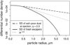 |
Fig. 11 Size distribution (arb. normalization) of the E ring particles in the vicinity of Enceladus evaluated from our model as those particles that escape Enceladus. The size distribution of the salt-poor dust grains in the model (at the moment of ejection from the sources on the tiger stripes) as well as a power law R−4.6 are shown for comparison. |
5 Results
We aimed to design a model that optimally fits all the available CDA data sets for the Enceladus plume. However, not all aspects of the model plume are equally important for the properties of the profiles of number density or composition. For instance, the existence of diffuse sources, with their wide ejection angles, emitting salt-rich dust is required to explain the early rise of the type III proportion in the E5 compositional profile (when the spacecraft was far away from the dense, central parts of the plume). In contrast, from the E17 profile we conclude that salt-rich dust contributes in total a relatively small fraction to the central plume above the SPT. Thus, the salt-rich dust contributes little or nothing to the number density profiles of E7 and E21 because of their horizontal flyby geometry that is similar to E17.
5.1 Profiles of particle number density
We evaluated the total dust production rate in the jets through the fits to the HRD number density profiles (Figs. 12 and 13). It is important to note that the in situ measurements are not sensitive to all the jets in the plume but only to those that are located close to the spacecraft’s ground track. Hence, making conclusions about the whole plume based on these measurements is an extrapolation. The width of the jets, that is, the parameter ω in the ejection direction distribution (Eq. (6)), plays a role in shaping the model number density profiles. Furthermore, if we consider tilted jets, their zenith angle and azimuth are also a factor for the amount of dust at a given point in space (see Fig. A.1).
In the model profiles of the E7 flyby the predicted number density rises sharply only when the spacecraft is directly above the SPT, while in the data we see a noticeable increase in the dust density already when Cassini was approaching Enceladus (see Fig. 2 for Cassini’s ground track). The HRD profiles from the low altitude flyby E2l show a fairly broad signal, corresponding to the plume as a whole, lacking clear peaks associated with the Tiger Stripe crossings (Fig. 6, compare also to Fig. 2). Conversely, the HRD profile from the E7 flyby (Fig. 5), crossing the plume at higher altitude than E2l, exhibits broad but clear peaks that correspond to the traversal of individual Tiger Stripes (Fig. 2). Thus, surprisingly, the structure of the sources manifests itself in the dust density more prominently at higher altitude. This finding is reversed in our model profiles of the two flybys, where the imprint of the sources is more pronounced at lower altitude, closer to the sources (Figs. 12 and 13). This discrepancy suggests that the directional distribution of dust emission from the sources may be more complex than assumed in our simple model. We discuss this point further in Sect. 6. We do not observe this flaw of extra structure in the compositional profiles (see Sect. 5.2) because Cassini’s ground track did not cross multiple tiger stripes during the E17 flyby, and the E5 ground track only crossed them when the spacecraft was at high altitudes. Cassini flew over the least active Alexandria at an altitude of 140 km and continued to rise steeply above the moon while crossing the other Tiger Stripes (see Figs. 1 and 2).
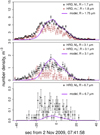 |
Fig. 12 Number density profile of the E7 flyby recorded by HRD counters M1, m′1, M2, m′2, and M3 and the model fits. The variability factor k = 1 (see Sect. 4.5). |
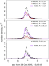 |
Fig. 13 Number density profile of the E7 flyby recorded by HRD counters M1, m′1, M2, m′2, and M3 and the model fits. The variability factor k = 1 (see Sect. 4.5). |
5.2 Compositional profiles
To model the compositional profiles of the Enceladus plume, we computed independently the number density of dust of the three compositional types along Cassini’s trajectory. Figures 14 and 15 show the comparison of the model results to the compositional profiles recorded by CDA.
Considering the variability of the plume quantified by Ingersoll & Ewald (2017) and Ingersoll et al. (2020), we modeled the E5 and E17 flybys with variability factors for the plume’s production rate of k = 2 and k = 1.7, respectively (see Sect. 4.5 and Table 3). These factors are applied to the production rate of the jets inferred from the HRD number density profiles and the production rate of the diffuse sources. The contribution by diffuse sources has little effect on the E17 compositional profile and it has practically no effect on the number density profiles of the E7 and E2l flybys. Eventually, our estimate for the production rate of the diffuse sources was obtained solely from the fit to the E5 compositional profile, where we applied the appropriate variability factor k = 2. Then the dust production rates of the diffuse sources during the E7, E 17, and E2l flybys are smaller, because the factor k is smaller for these flybys.
In order to assess if such a variability of the plume is actually required by the CDA data, we fitted a model in which the plume activity is kept constant. Results for this case are also shown in Figs. 14 and 15. It corresponds to a value of k = 1 for the E5 and E17 flybys, so that the plume emits as much dust during these flybys as it does during the E7 and E2l flybys. The proportion of the three types of dust in the E5 profile before closest approach is largely defined by the number density of the diffusely ejected dust relative to the E ring background density. Therefore, the model compositional profile is the most sensitive to the total production rate of the plume, and we observe the largest difference between the variable and non-variable models in the E5 profile before closest approach. However, when fitting the models to the all CDA data the difference between the cases remains within the measurement errors (Figs. 14 and 15). Hence, we conclude that although our modeling could be compatible with temporal variable in the plume, our fits do not require it.
The total production rate of the plume determines the range where the compositional profiles inside the plume blend over to their respective levels in the E ring. In the E17 profile we considered the data points around ±60 sec from closest approach to represent the E ring backround composition. In the E5 profile the E ring background is seen in the data prior to −60 sec from closest approach. At the spacecraft position at +60 sec of the E5 flyby the density of plume dust estimated by the model is still high compared to the dust of the E ring background.
In the E5 compositional profile the diffuse salt-rich cloud causes the early rise of type III proportion. This rise is less pronounced in the model profile of E17 because the size distribution of the salt-rich dust has a rather narrow peak that lies below the range to which the slow E17 flyby is sensitive to. Also, the small value adopted for the parameter Rc (see Eq. (4)) makes those salt-rich grains that would be large enough to be detectable during E 17, rise only to altitudes that remain mostly below the altitude of the spacecraft’s closest approach.
The decadal variability inferred by Ingersoll & Ewald (2017) suggests a rate of plume activity that was lower in 2012 than in 2008. This helps reach a better agreement with the data because a reduced production rate at the time of E 17, relative to E5 (see Sect. 4.5), allows the model profile to return to the background E ring composition levels already at a shorter distance from closest approach.
Neither the drop to zero of the type III proportion at -20 sec nor the peak of the type II proportion around +45 sec in the E5 compositional profile are reproduced by our model. These features may indicate local variations of dust production and composition over the SPT. In the Appendix in Fig. A.8 we present a modification of the model to match the type II peak, exploring the possibility that the necessary amount of type II dust could be supplied by a very narrow jet. For instance, the jet III from Spitale & Porco (2007) is situated very close to Cassini’s ground track at this moment.
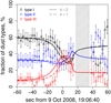 |
Fig. 14 E5 compositional profile measured (symbols) and modeled (lines) comparing the cases with (k = 2) and without (k = 1) and taking into account the plume’s variability. |
Total dust production rate of the plume.
5.3 Total dust production rate
Table 4 shows the mass production rate of the entire plume inferred from our analysis, obtained with the assumption that the particles are spherical with a bulk density of 920 kg m−3. The values in Table 4 correspond to the activity levels of E7 and E21, that is, using k = 1. Rates for the time at which the E5 profile was recorded can be obtained with k = 2, and for the time of E17 with k = 1.7.
These mass production rates are obtained using 0.1 µm and 15 µm as the lower and upper cutoff radii for the size distributions of salt-poor and salt-rich grains (Eqs. (7) and (8)). The value for the minimal grain size does not affect the estimate for the mass production rate. The maximal size is important. The value of 15 µm is a lower limit for the maximal grain size inferred from the largest thresholds of HRD that were triggered in all flybys. A larger maximum particle size would not change much the salt-rich mass production rate, because this type of grains possesses a fairly narrow distribution in form of a log-normal that is naturally confined to smaller sizes. However, a larger maximum particle size would make a significant difference for the salt-poor dust that is in our model a power law with negative slope 2.3. For instance, increasing the upper limit somewhat to 18 µm would result in 39 kg of salt-poor dust produced every second, and an unrealistically high production rate of 300 kg s−1 would be obtained for an upper cutoff above 60 µm. It is possible, however, that beyond the size threshold of the M3 counter of the E7 flyby the size distribution of salt-poor dust becomes steeper than 2.3. We cannot assess the size distribution in this size range from our data. Thus, the numbers in the Table 4 are the minimal mass production rates necessary to fit the CDA data. The proportion of salt-rich dust in the plume is only 0.3% by mass because the salt-rich particles in our model are small. This is supported by evidence from E ring measurements suggesting that type III particles are, on average, smaller than type II grains (Nölle et al. 2024).
When fitting our model to the data, we applied the condition that the total dust mass production rate remains a reasonably small fraction of the gas mass production rate. This is motivated by the physical requirement that the gas must accelerate and transport the dust through the subsurface vents and ultimately pushes the dust into space. If the dust mass becomes too large, then the gas cannot efficiently accelerate the dust to the observed velocities. In this sense, the dust mass production rate is treated as a constraining parameter in our model. Estimates of the gas production rate range from 300 kg s−1, based on UVIS measurements that show only moderate plume variability (Hansen et al. 2020), to 900 kg s−1 derived from INMS measurements (Smith et al. 2010; Yeoh et al. 2017). In the INMS data pronounced variability of the plume is seen and the 900 kg s−1 correspond to the most active phase. With the size and ejection speed distributions adopted in our model (see Sect. 4), the obtained mass production rate of about 28kg s−1 falls plausibly in the range of previous estimates: 5 kg s−1 (Schmidt et al. 2008), 51 ± 18 kg s−1 (Ingersoll & Ewald 2011), 12–50 kg s−1 (Meier et al. 2014), 12 kg s−1 (Meier et al. 2015), and 29 ± 7 kg s−1 (Porco et al. 2017).
5.4 Model plume spatial structure
In this section we examine in more detail the structure of the Enceladus plume according to the constructed model. We analyze the spatial distribution of different types of dust above the SPT. As throughout this paper, we exclude salt-poor particles bearing complex high-mass organic compounds from our consideration (see Sect. 2.1 for details).
Figure 16 displays the distribution of dust evaluated on segments of spherical surfaces at different altitudes above the SPT. We show the dust mass integrated over the size distributions over the whole range of sizes considered (0.1–15 µm). The model exhibits density drops between the Tiger Stripes, which are more pronounced at lower than at higher altitudes. We pointed out a similar tendency in the HRD number density profiles (see Sect. 5.1). Possible reasons are discussed in Sect. 6.
We evaluate in Fig. 17 the mass of plume dust that could be collected by a detector on a spacecraft traversing the plume on a hypothetical horizontal trajectory marked as dashed lines in Fig. 16. The detector of 1 m2 area is pointing in apex direction of the spacecraft motion. The collected mass is given separately for the salt-rich and salt-poor dust for each altitude that is shown in Fig. 16.
In Fig. 17 we do not discriminate between particles of type I and type II because, when a salt-poor particle is detected it in principle always contains organics and only the appearance of organic lines in the spectrum (making it type II) would depend on grain size, impact velocity, and the characteristics of the detector (see discussion in Sect. 2.1). However, if we assume that instruments onboard future space missions will, similarly to the CA, detect organics only in sufficiently large particles, then we may use the grains’ mean radius as a metric for the expected type II dust proportion in the salt-poor dust. To this end, Fig. 18 shows the mean radius of salt-poor and salt-rich grains in our model versus altitude (computed along the dashed lines in Fig. 16). We find that the salt-poor dust population shows a significant decrease in the mean grain radius with altitude, the abundant, large salt-poor particles contributing more to the dust population at lower altitudes. We suggest that this is the reason for the trend seen in the E17 compositional profile, where the type II proportion (containing organics) peaks near the closest approach.
The salt-rich grains are relatively small since their radii are confined to a narrow range (Fig. 9). As a result, most of these grains are ejected at high speeds (a large fraction even above Enceladus’ escape velocity). For this reason the variation of the mean size of salt-rich grains with altitude in the plume is mild.
The gas production rate in the Enceladus plume is not used explicitly as a parameter in our model. However, our model and the estimate for the dust production is implicitly based on the assumption that the gas dominates the momentum budget of the plume. In order to derive constraints on the variation of the ratio of dust-to-gas in the Enceladus plume, we assumed that the overall production of dust must be on the order of 10% or less of the gas. With this initial ratio, we calculated how the dust-togas ratio changes with altitude. Intuitively, one expects a higher gas production rate in the jets than in the diffuse sources, as the gas flux in the jets is twice faster and carries nearly 1000 times more solid material. Based on this, we roughly estimated the gas production rate of the whole plume as 330 kg s−1 of which 300 kg s−1 are equally distributed among the 100 jets and 30 kg s−1 among the diffuse sources. Thus, the initial dust-to-gas ratio in the diffuse sources is much lower than in the jets. We evaluated the gas density spatial distribution using the same approach as for the calculation of dust density, namely the two-body model by Ershova & Schmidt (2021) and the DUDI code. We modeled the dynamics of water vapor molecules as dust grains. We employed the same ejection direction distribution as for the dust ejection (see Sect. 4.3 and Table 3). The ejection speed distributions of the jets and the diffuse sources were set to be uniform within a 60 m s−1 range centered at the gas speed values specified for the diffuse sources and jets in Table 3.
Figure 19 shows the dust-to-gas mass ratio in our model, evaluated in a plane that contains the moon center and the hypothetical flyby trajectories considered in Figs. 16 and 17. This plane is nearly normal to the TSs. Gas is ejected at speeds much higher than the escape velocity of Enceladus, and no E ring background for the gas is considered. Because of this, there is a region where our model reaches zero gas density (light-gray in Fig. 19). Similarly to Hedman et al. (2018), who analyzed variations in gas-to-dust ratio based on VIMS, UVIS, INMS, and RPWS observations, we obtained a decreased dust-to-gas ratio on Alexandria’s side of the plume than on the Damascus’ side, though the difference we obtain is not as large as in Hedman et al. (2018). The reason for this difference is that fewer jets are located on Alexandria. However, the asymmetry of the model plume in Fig. 19 is not as extreme as reported by Hedman et al. (2018), whose high numbers cannot be achieved with our assumption that (by mass) ten times less dust is ejected than gas. The dust-to-gas mass ratio is higher between the TSs than strictly above them because these regions are traversed by the massive, slow particles falling back to the moon.
Finally, we look at the plume’s composition in general. We display in Fig. 20 the proportion of salt-rich dust evaluated in the same plane that was used for Fig. 19. Again, the E ring background is not taken into account, so the figure shows the spatial compositional variations of the dust in the plume alone. The quantity shown in Fig. 20 is obtained for the whole range of particle sizes for which the model size distributions are defined, that is, 0.1–15 µm for both salt-poor and salt-rich dust grain radii. Thus, the numbers in Fig. 20 generally differ from the compositional profiles of the E5 and E17 flybys because these flybys sample only a part of the full size distribution (Figs. 9 and 10). The region directly above the SPT is dominated by dust from the jets. The fraction of type III grains reaches a nearly constant value at sufficiently high altitude, remaining close to the respective value at ejection (see Table 3). This is a consequence of the high ejection velocity in the jets. In contrast, the diffusely ejected salt-rich dust is more abundant at lower latitudes. It is never equal to 100% because there are salt-poor particles on bound orbits with small or moderate eccentricities and the ones ejected with a small angle to the horizon (see Sect. 4.3 for the discussion of the ejection angle distribution). The salt-rich dust found at low latitudes comes almost exclusively from diffuse sources, as the small salt-rich particles ejected by the jets escape Enceladus due to their high speeds (see Sect. 4.2 for the discussion of the ejection speed distribution). Most of the orbits of salt-poor particles reaching low latitudes are characterized by high energies, allowing these particles to reach high altitudes, pass their aphelion (see Sect. 2.2 of Ershova & Schmidt 2021, for details on possible trajectories of dust grains), and fall back to the moon at an angle to the surface normal equal to π – ψ, where ψ is the particle’s ejection velocity angle to the surface normal. The angle ψ tends to be small for the jets, while for the diffuse sources, any value of ψ is almost equally probable (see Sect. 4.3). As a result, the nearly horizontal contours at low latitudes in Fig. 20 reflect the distribution of orbital energies of the salt-poor particles that lead to salt-poor dust falling back to Enceladus with a small angle to the surface normal.
 |
Fig. 16 Density of dust at different altitudes above the SPT of Enceladus. The red cross marks the south pole. The dashed lines denote the ground tracks of hypothetical horizontal flybys (see text). |
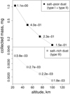 |
Fig. 17 Prediction of our model for the total mass of salt-rich and salt-poor dust collected during hypothetical horizontal flybys (performed along the dashed lines shown in Fig. 16). The mass is calculated for an ideal plane detector of 1 m2 area. Masses for types I and II are added together, giving the salt-poor dust mass. All salt-poor dust particles contain organic compounds, although the actual proportion of mass-spectra showing lines of organics (which classifies them as type II) may depend on the instrument characteristics and flyby velocity. |
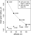 |
Fig. 18 Prediction of our model for the mean radius of salt-rich and salt-poor dust particles encountered on the average along the hypothetical flybys considered in Fig. 17 (dashed lines shown in Fig. 16). |
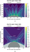 |
Fig. 19 Dust-to-gas mass ratio distribution in the plane along the dashed line in Fig. 16 and the center of Enceladus. The light gray area depicts the region that the freshly ejected gas does not reach. The rectangle in panel b marks the region shown in panel a. |
6 Summary and discussion
We have analyzed the data that the Cassini CDA collected in situ in the Enceladus plume. These data are profiles of particle count rates recorded by the HRD subsystem during plume crossings at the Enceladus flybys E7 and E2l. The different channels of the HRD yield information on the number density of different grain sizes and their variation in the plume. However, we also used profiles of relative abundances of grains of different compositional types (type I: salt-poor without organics; type II: salt-poor with organics; type III: salt-rich) that were recorded by the DA subsystem during flybys E5 and E17. The data from the E5 flyby were analyzed previously by Postberg et al. (2011).
We put the different types of data in a common framework in terms of fits to a new model for the Enceladus dust plume that is based on the mathematical description of dust ejection developed by Ershova & Schmidt (2021). This model employs two types of sources of dust on the SPT that differ in composition and the velocity distribution of the emitted dust. The “diffuse sources” are all distributed along the TSs fractures on the SPT. They emit salt-rich dust that is derived from droplets that exist above a table of liquid water at some depth (Postberg et al. 2011). We identified the “jet sources” emitting dust at larger velocities in a more narrowly confined configuration with the jets derived by Porco et al. (2014) from imaging. In addition to salt-rich dust, the jets emit salt-poor dust that condenses from the gas abundantly when high levels of supersaturation are reached in supersonic flow. The HRD measurements are primarily used to constrain the dust production rates in the model as well as the dust size distribution. The compositional profiles from E5 and E17 give information on the variation of compositional types with altitude and detection location over the SPT. Since the stratification of dust in the plume derives from the ejection velocity that is sensitive to the grain size and mass via the coupling to the gas (see Sect. 4.2), the compositional profiles of the model constrain certain combinations of sizes and ejection velocities for the different compositional types.
The application of the dust plume model to the data is complicated by the fact that the flybys occurred with very different relative velocity to Enceladus so that the impact velocity of grains on the detector was different. For a higher impact velocity, the detectors are sensitive to lower grain sizes and the corresponding shift in the sensitivity ranges for HRD and DA that we consider in our model. In addition, for the compositional data from E5 and E17, we took into account recent advances in the understanding of the CDA mass spectra, leading us to a revised interpretation of the compositional types I and II.
The grains of types I and II in principle represent particles of the same (salt-poor) composition. But the organics in these grains become detectable in the CDA spectra only for sufficiently large grains (Postberg et al. 2018b; Khawaja et al. 2019). As a result, the organic bearing type II grains are larger than the type I particles, which is reflected in the model by an impact velocity dependent boundary between these two types. But as representatives of the same salt-poor population, the type I and II grains still obey the same size distribution. Moreover, we considered the observation from lab experiments that the ion yield of a particle in an impact ionization event depends on the composition of the grain (Wiederschein et al. 2015). Since DA records useful mass spectra only for a given range of the ion yield, we inferred for different compositional types a different range of grain sizes to which the instrument is sensitive at E5 and E17, respectively. Salt-rich particles (type III) have a larger ion yield than the salt-poor particles (type I and II). Thus, for the same measured ion yield, a salt-rich dust particle is smaller than a salt-poor dust particle.
Our simulation does not consider the type 2 grains exhibiting substantial amounts of refractory organics of high molecular mass because of the lack of plume data of this type (see Sect. 2.1 for details on type II HMOC). The modeled compositional profiles do not make a prediction about these rare particles that are probably of high astrobiological interest. In the future, we might attempt to include these ice grains into the model after the revised analysis of both E5 and E ring data that is currently in progress.
The flyby E5 in 2008 was special in two ways. It was highly inclined with respect to the orbital plane of Enceladus, and it had the highest relative velocity of all Enceladus flybys. In contrast, the E17 flyby in 2012 was a nearly horizontal traversal of the SPT with a much lower relative velocity. At E5, a drastic increase in the frequency of salt-rich particles was observed (Postberg et al. 2009) after the closest approach of the spacecraft (which happened at relatively low southern latitudes), while at the spacecraft’s closest approach above the SPT during E17, the increase in the proportion of salt-rich grains was much shallower, and their fraction stayed well below the abundance of the salt-poor compositional types. Reproducing the compositional profiles from E5 and E17 simultaneously is only possible if most of the salt-rich dust is smaller than the lower size threshold for detections during the low-velocity flyby of E17. This is the reason why salt-poor dust dominates the E17 compositional profile. The same must be true for the HRD flybys E7 and E21 that have a similarly slow encounter speed and horizontal geometry (for which no compositional profiles were recorded). Therefore, the number density profiles obtained with the HRD for these flybys serve as constraints only for the abundance and size distribution of the salt-poor grains.
In our model, the salt-poor dust is ejected from numerous jets (Porco et al. 2014) along the TSs, and it reaches the high altitudes sampled at E7 and E21 because of the relatively large ejection velocities established in the jets. The HRD profiles exhibit peaks in number density corresponding to TS crossings at a rather higher altitude (E7 with 100 km closest approach), while these peaks are practically absent in the E21 profile below the 50 km altitude. The profiles compiled from our model show the opposite trend (see Sect. 5.1 and Fig. 16 in Sect. 5.4). In the model, in contrast, peaks of number density directly above the sulci (and the troughs between them) are sharper at lower altitudes and closer to the sources. This difference likely arises from the simplifications in the parameterization of the dust ejection made in the model. An additional diffuse mode of ejection from the TSs of salt-poor dust, with low ejection velocities, would lead to a smoother signal at low altitudes, while the faster, more collimated jets reach larger altitudes and thus stand out in the measurement of E7. Further factors that might affect the precise form of the HRD profiles are the detailed orientations of the large number of sources, the variation of their dust production rates along the TSs, the ejection velocity, and variations in the width of the vents.
We find that for freshly ejected salt-poor dust, a power-law size distribution with a slope of negative 2.3 (Eq. (7)) is consistent with the data. This is a rather flat distribution, and thus, the upper size cutoff is important for determining the total dust mass production rate of the plume (see Sect. 5.3). Unfortunately, the available data do not allow us to directly evaluate this upper size limit because such large particles hardly reach the altitudes of the Cassini flybys. However, we can use the largest grain size detected by HRD during the flybys to derive a lower limit for the mass production rate. At E7, the HRD detected two grains larger than about 13 µm. By using 15 µm as the cutoff radius for the size distribution (of all grains of any compositional type), we obtained a lower limit of 28 kg s−1 for the mass production rate of salt-poor dust in the plume, which includes nearly pure water ice (type I) and organic bearing particles (type II). The estimate is very sensitive to the assumed cutoff radius. For instance, using 20 µm as the cutoff size already doubles the salt-poor dust mass production rate.
For the size distribution of the salt-rich particles, we found a consistent fit in terms of a log-normal distribution (Eq. (8)) with a relatively narrow peak at approximately 0.3 µm. This implies that the mass production rate for salt-rich dust is only about 0.3% of the total mass production rate of the plume.
These rates are derived from fits to the HRD data obtained during flybys E7 and E21. From imaging data, there exists evidence that the plume produced more dust during the times of the E5 and E17 flybys (Ingersoll & Ewald 2017; Ingersoll et al. 2020). From the CDA data, we can neither confirm nor refute such a variability.
From the parametrization of the ejection physics (size-distributions, velocity distributions, gas velocity, strength of gas-to-grain coupling) as well as from the location and properties of sources (position on the SPT, individual activity rates, jet orientation, and opening angle), our model necessarily possesses an uncomfortably large number of parameters. Technically, these cannot be all constrained fully from fits to the data. Instead, we have fixed certain parameters to plausible numbers derived in the literature (such as gas velocities and jet location). Other parameters affect the model (approximately, not exactly) in groups so that their variation can be (roughly) canceled out by a respective variation of another parameter. This is, for instance, the case for the gas velocity, gas density, and grain size. Thus, the parameter sets we have adopted to fit our model do not strictly represent a unique solution; they are our best estimate at this point. However, favorable aspects of our model include the fact that it is self-consistent and that the measurement constraints come from very complementary data sets. The narrow peak of the salt-rich size distribution outside the detectable grain size range of the E17 flyby is necessary to simultaneously match the low fraction of type III grains in the E17 compositional profile and the high fraction of the type III in the E5 profile. A satisfactory fit to the observational data can only be achieved if the production of salt-rich dust in the plume is less than 1% by mass. Thus, our results lead to very different conclusions than the earlier work of (Postberg et al. 2011) on the relative contribution of the compositional types to the plume mass. The analysis of Postberg et al. (2011) was based on the E5 compositional profile alone, and it was based on the (at that time plausible) conjecture that salt-rich dust should be larger and more massive than the salt-poor type in order to reproduce the enrichment of this type at low plume altitudes. This model, however, would lead to a dominance of salt-rich dust around the closest approach of E17, which is not seen in the data.
In the new model proposed here, it is the diffuse plume sources with lower gas velocities and wider ejection angles that lead to the E5 enrichment of salt-rich grains. Although salt-rich dust is seen nearly everywhere in the plume, the diffuse salt-rich cloud is dominant only in the fringe of the plume, which is traversed by Cassini after the closest approach of the E5 flyby. In contrast, the high-velocity jets only produce salt-poor particles. This naturally leads to a much lower mass production of salty grains of less than 1% in total and, compared to previous work, a larger fraction of salt-poor but organic-enriched ice grains in the dense central part of the plume.
Finally, we note that although we considered the inferred overall variation of plume productivity with the orbital phase as well as long-term trends (Hedman et al. 2013; Ingersoll & Ewald 2017; Ingersoll et al. 2020), we did not investigate with our model the possibility of the plume experiencing complex variations with time. This would increase the number of parameters of the model beyond any reasonable level. In other words, our data are insufficient to constrain such plume variability in a reliable manner. For instance, it is unclear if the diffuse component and the jets vary their activity proportionally. Also, we do not consider the possibility of a more dynamical structure of the plume, such as jets emerging and disappearing between the flybys. With our sparse in situ data, it is hard or impossible to tell apart such temporal variations from local variations in a steady plume. We reproduced with our model the main trends without paying too much attention to the fine structure of the plume.
In the future, it appears to be a fruitful endeavor to further constrain our plume model in detail using ISS images and VIMS data cubes. The software package DUDI (Ershova & Schmidt 2021) can be freely downloaded from GitHub3. The package allows the user to efficiently construct synthetic images, such as Figs. A.5–A.7, that can be combined with photometric modeling in order to take into account the effect of light scattering.
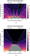 |
Fig. 20 Salt-rich dust percentage in the same plane as Fig. 19. The proportion has been computed for the whole range of grain sizes used in the model: 0.1–15 µm for both salt-poor and salt-rich dust particles. The rectangle in panel b marks the region shown in panel a. |
Acknowledgments
This work was supported by the Academy of Finland (A.E. and J.S.). F.P., N.K., and L.N. were supported by the European Research Council (ERC) under the European Union’s Horizon 2020 research and innovation programme (Consolidator Grant 724908-Habitat OASIS). The authors thank the anonymous reviewer for their careful attention to this paper and for the many useful suggestions for its improvement.
Appendix A Variation of jet parameters
To investigate the dependence of the model results on the characteristics of the jets, we vary the width, positions and orientations of the jets. These parameters play an important role in reproducing the HRD profiles of number density. Conversely, the compositional profiles exhibit less sensitivity to variations in jet parameters. This is attributed to their lower spatial resolution and the presence of all compositional dust types within the jets.
In our primary model setup presented in this paper, we utilized the jet locations as determined by Porco et al. (2014). However, we neglected the measured tilts of the jets, instead employing jet axes that remain normal to the surface. To assess the sensitivity of the model outcomes to the tilt angles and the positions of the jets, we test two alternative setups. Firstly, we retained the original reported positions of the jets along with their non-zero zenith angles and azimuths (Porco et al. 2014). Secondly, we implemented 80 vertical jets evenly distributed along the Tiger Stripes. Figure A.1 illustrates the model profiles for the HRD flybys obtained using these three setups, all normalized to maintain the same total mass production of the plume. Generally, employing the jet positions from Porco et al. (2014) yields better alignment with the features observed in the profiles. Notably, for the E21 model profile, utilizing the original tilts of the jets results in a somewhat improved agreement.
However, the inclination of the jets also plays a role for the E17 compositional profile. Figure A.3 shows the effect of taking into account the jets’ tilts for the Porco et al. (2014) sources. The profile that uses the full tilts is flatter, providing a worse agreement with the data especially at larger distance from closest approach. The fairly large zenith angles that many jets in the list of Porco et al. (2014) possess supply more plume dust to the space distant from the SPT. The E5 compositional profile is insensitive to the variation of tilts in the model (Fig. A.2). The fact that the E17 profile model agreement with the data becomes worse when the jets’ tilts are taken into account implies that such jets were not present close to Cassini’s trajectory at the time of the flyby. However, we cannot exclude the existence of the highly tilted jets on the Damascus’s side of the SPT.
Another degree of freedom is the width of the jets (parameter ω in Eq. (6)). Our nominal model uses a value of ω = 10° throughout. Figure A.4 shows the profiles obtained with more confined jets (ω = 5°). The total mass production of the plume is kept the same. The model profiles in this case look more peaked, and although the high peak of the E21 profile is reproduced better with the narrower jets, we conclude that the wider jets give a better qualitative agreement with the data. Wider jets are preferable if we compare not the peaks in the observed and modeled profiles but the total number of particles recorded during the flyby.
We show in Figs. A.5–A.7 how jets with different width ω could look in imaging. Some images of Enceladus active south pole strongly witness the presence of very confined jets in the model, for example, Fig. 1a of Porco et al. (2014). However, Fig. 1b in the same paper has a dust jet with a significantly larger opening angle. The results of our modeling do not deny existence of very narrow jets. It is possible that they represent a minority of the population. A wide jet can also be seen as an approximation for an ensemble of confined jets that are randomly tilted.
Finally, we demonstrate the potential importance of short scale local variations in the plume to matching detailed features of the compositional profiles. In Fig. A.8 we reproduced the peak of the type II proportion recorded at about +45 seconds by introducing one additional vertical jet at −81.3° N.L. 292.8° E.L. (the position of the jet III from Spitale & Porco (2007)). In order to match the peak as it is shown in Fig. A.8, this jet must eject solely type II dust with a rate that is three times higher than for the other jets in the model. It also has been given a more narrow ejection direction distribution (Eq. (6) with ω = 3°) to match the peak in the data. This may witness for complex differences in ejection dynamics over the STP of Enceladus.
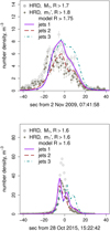 |
Fig. A.1 Number density profiles of the E7 (upper panel) and E21 flybys (lower panel). Comparison of three model setups for the jets: jets 1 — jets from Porco et al. (2014) neglecting tilts; jets 2 — tilted jets from Porco et al. (2014); jets 3 — vertical jets uniformly distributed along the TSs. |
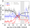 |
Fig. A.2 E5 compositional profile measured (symbols) and modeled (lines) using the jet sources from Porco et al. (2014). The solid line corresponds to a model that uses the original tilts for the jets as reported in Porco et al. (2014). The dashed line corresponds to a model that neglects these tilts and uses a vertical jet axis instead. |
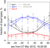 |
Fig. A.3 E17 compositional profile measured (symbols) and modeled (lines) using the jet sources from Porco et al. (2014). The solid line corresponds to a model that uses the original tilts for the jets as reported in Porco et al. (2014). The dashed line corresponds to a model that neglects these tilts and uses a vertical jet axis instead. |
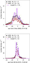 |
Fig. A.4 Number density profiles of the E7 (upper panel) and E21 (lower panel) flybys. Jets from Porco et al. (2014) with more confined ejection than used in the model settings (Eq. (6) with ω = 5°). |
 |
Fig. A.5 Jet with ω = 3°. |
 |
Fig. A.6 Jet with ω = 5°. |
 |
Fig. A.7 Jet with ω = 10°. |
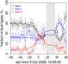 |
Fig. A.8 E5 compositional profile measured (symbols) and modeled (lines) with a narrow jet ejecting only type II dust with the rate three times higher than the other jets in our model dust added at −81.3° NL 292.8° WL. |
References
- Berne, A., Simons, M., Keane, J. T., & Park, R. S. 2023, J. Geophys. Res. Planets, 128, e2022JE007712 [NASA ADS] [CrossRef] [Google Scholar]
- Dong, Y., Hill, T. W., Teolis, B. D., Magee, B. A., & Waite, J. H. 2011, J. Geophys. Res., 116, 10204 [NASA ADS] [Google Scholar]
- Dougherty, M. K., Khurana, K. K., Neubauer, F. M., et al. 2006, Science, 311, 1406 [NASA ADS] [CrossRef] [Google Scholar]
- Dougherty, M. K., Buratti, B. J., Seidelmann, P. K., & Spencer, J. R. 2018, in Enceladus and the Icy Moons of Saturn, eds. P. M. Schenk, R. N. Clark, C. J. A. Howett, A. J. Verbiscer, & J. H. Waite (Tucson: University of Arizona Press), 3 [Google Scholar]
- Ershova, A., & Schmidt, J. 2021, A&A, 650, A186 [NASA ADS] [CrossRef] [EDP Sciences] [Google Scholar]
- Feibelman, W. A. 1967, Nature, 214, 793 [NASA ADS] [CrossRef] [Google Scholar]
- Haff, P. K., Eviatar, A., & Siscoe, G. L. 1983, Icarus, 56, 426 [NASA ADS] [CrossRef] [Google Scholar]
- Hand, K. P., Sotin, C., Hayes, A., & Coustenis, A. 2020, Space Sci. Rev., 216, 1 [CrossRef] [Google Scholar]
- Hansen, C. J., Esposito, L. W., Stewart, A. I. F., et al. 2006, Science, 311, 1422 [NASA ADS] [CrossRef] [Google Scholar]
- Hansen, C. J., Esposito, L. W., Stewart, A. I. F., et al. 2008, Nature, 456, 477 [NASA ADS] [CrossRef] [Google Scholar]
- Hansen, C. J., Esposito, L. W., Colwell, J. E., et al. 2020, Icarus, 344, 113461 [CrossRef] [Google Scholar]
- Hedman, M. M., & Young, M. 2021, The Planetary Science Journal, 2, 127 [NASA ADS] [CrossRef] [Google Scholar]
- Hedman, M. M., Nicholson, P. D., Showalter, M. R., et al. 2009, ApJ, 693, 1749 [NASA ADS] [CrossRef] [Google Scholar]
- Hedman, M. M., Gosmeyer, C. M., Nicholson, P. D., et al. 2013, Nature, 500, 182 [NASA ADS] [CrossRef] [Google Scholar]
- Hedman, M. M., Dhingra, D., Nicholson, P. D., et al. 2018, Icarus, 305, 123 [NASA ADS] [CrossRef] [Google Scholar]
- Hemingway, D. J., Rudolph, M. L., & Manga, M. 2020, Nat. Astron., 4, 234 [Google Scholar]
- Howett, C. J. A., Spencer, J. R., Pearl, J., & Segura, M. 2011, J. Geophys. Res., 116, E03003 [Google Scholar]
- Howett, C., Nimmo, F., & Spencer, J. 2022, European Planetary Science Congress, 219 [Google Scholar]
- Hsu, H.-W., Postberg, F., Sekine, Y., et al. 2015, Nature, 519, 207 [Google Scholar]
- Ingersoll, A. P., & Ewald, S. P. 2011, Icarus, 216, 492 [NASA ADS] [CrossRef] [Google Scholar]
- Ingersoll, A. P., & Ewald, S. P. 2017, Icarus, 282, 260 [NASA ADS] [CrossRef] [Google Scholar]
- Ingersoll, A. P., Ewald, S. P., & Trumbo, S. K. 2020, Icarus, 344, 113345 [NASA ADS] [CrossRef] [Google Scholar]
- Kargel, J. S., & Pozio, S. 1996, Icarus, 119, 385 [NASA ADS] [CrossRef] [Google Scholar]
- Kempf, S. 2008, Planet. Space Sci., 56, 378 [NASA ADS] [CrossRef] [Google Scholar]
- Kempf, S., Beckmann, U., Moragas-Klostermeyer, G., et al. 2008, Icarus, 193, 420 [CrossRef] [Google Scholar]
- Kempf, S., Beckmann, U., & Schmidt, J. 2010, Icarus, 206, 446 [CrossRef] [Google Scholar]
- Kempf, S., Srama, R., & Graps, A. 2012, The Cosmic Dust Analyser Data Handbook, https://sbn.psi.edu/pds/resource/cdaDataHB-5-4-17.pdf [Google Scholar]
- Khawaja, N., Postberg, F., Hillier, J., et al. 2019, MNRAS, 489, 5231 [Google Scholar]
- Kite, E. S., & Rubin, A. M. 2016, Proc. Natl. Acad. Sci., 113, 3972 [NASA ADS] [CrossRef] [Google Scholar]
- Le Gall, A., Leyrat, C., Janssen, M. A., et al. 2017, Nat. Astron., 1, 0063 [NASA ADS] [CrossRef] [Google Scholar]
- Martens, H. R., Ingersoll, A. P., Ewald, S. P., Helfenstein, P., & Giese, B. 2015, Icarus, 245, 162 [NASA ADS] [CrossRef] [Google Scholar]
- McKay, C. P. 2020, Astrobiology, 20, 163 [NASA ADS] [CrossRef] [Google Scholar]
- Meier, P., Kriegel, H., Motschmann, U., et al. 2014, Planet. Space Sci., 104, 216 [NASA ADS] [CrossRef] [Google Scholar]
- Meier, P., Motschmann, U., Schmidt, J., et al. 2015, Planet. Space Sci., 119, 208 [NASA ADS] [CrossRef] [Google Scholar]
- Mitchell, C. J., Porco, C. C., & Weiss, J. W. 2015, AJ, 149, 156 [NASA ADS] [CrossRef] [Google Scholar]
- Napoleoni, M., Klenner, F., Hortal Sanchez, L., et al. 2023a, ACS Earth Space Chem., 7, 1675 [NASA ADS] [CrossRef] [Google Scholar]
- Napoleoni, M., Klenner, F., Khawaja, N., Hillier, J. K., & Postberg, F. 2023b, ACS Earth Space Chem., 7, 735 [NASA ADS] [CrossRef] [Google Scholar]
- Nimmo, F., Porco, C., & Mitchell, C. 2014, AJ, 148, 46 [NASA ADS] [CrossRef] [Google Scholar]
- Nölle, L. 2022, PhD thesis, Freie Universitaet Berlin, Germany [Google Scholar]
- Nölle, L., Postberg, F., Schmidt, J., et al. 2024, MNRAS, 527, 8131 [Google Scholar]
- Pang, K. D., Voge, C. C., Rhoads, J. W., & Ajello, J. M. 1984, J. Geophys. Res., 89, 9459 [NASA ADS] [CrossRef] [Google Scholar]
- Porco, C. C., Helfenstein, P., Thomas, P. C., et al. 2006, Sci., 311, 1393 [NASA ADS] [CrossRef] [Google Scholar]
- Porco, C., DiNino, D., & Nimmo, F. 2014, AJ, 148, 45 [NASA ADS] [CrossRef] [Google Scholar]
- Porco, C., Nimmo, F., & DiNino, D. 2015, AGU Fall Meeting Abstracts, 2015, P13A [Google Scholar]
- Porco, C. C., Dones, L., & Mitchell, C. 2017, Astrobiology, 17, 876 [NASA ADS] [CrossRef] [Google Scholar]
- Portyankina, G., Esposito, L. W., Aye, K.-M., Hansen, C. J., & Ali, A. 2022, Icarus, 383, 114918 [NASA ADS] [CrossRef] [Google Scholar]
- Postberg, F., Kempf, S., Hillier, J. K., et al. 2008, Icarus, 193, 438 [NASA ADS] [CrossRef] [Google Scholar]
- Postberg, F., Kempf, S., Schmidt, J., et al. 2009, Nature, 459, 1098 [Google Scholar]
- Postberg, F., Schmidt, J., Hillier, J. K., Kempf, S., & Srama, R. 2011, Nature, 474, 620 [NASA ADS] [CrossRef] [Google Scholar]
- Postberg, F., Clark, R. N., Hansen, C. J., et al. 2018a, in Enceladus and the Icy Moons of Saturn, eds. P. M. Schenk, R. N. Clark, C. J. A. Howett, A. J. Verbiscer, & J. H. Waite (Cambridge: Cambridge University Press), 129 [Google Scholar]
- Postberg, F., Khawaja, N., Abel, B., et al. 2018b, Nature, 558, 564 [Google Scholar]
- Postberg, F., Sekine, Y., Klenner, F., et al. 2023, Nature, 618, 489 [NASA ADS] [CrossRef] [Google Scholar]
- Schmidt, J., Brilliantov, N. V., Spahn, F., & Kempf, S. 2008, Nature, 451, 685 [NASA ADS] [CrossRef] [Google Scholar]
- Sharma, H., Hedman, M. M., & Vahidinia, S. 2023, The Planetary Science Journal, 4, 108 [NASA ADS] [CrossRef] [Google Scholar]
- Showalter, M., Cuzzi, J., & Larson, S. 1991, Icarus, 94, 451 [CrossRef] [Google Scholar]
- Smith, B., Cook, A. F., Feibelman, W. A., & Beebe, R. 1975, Icarus, 25, 466 [CrossRef] [Google Scholar]
- Smith, H. T., Johnson, R. E., Perry, M. E., et al. 2010, J. Geophys. Res., 115, 10252 [NASA ADS] [Google Scholar]
- Southworth, B. S., Kempf, S., & Spitale, J. 2019, Icarus, 319, 33 [NASA ADS] [CrossRef] [Google Scholar]
- Spahn, F., Schmidt, J., Albers, N., et al. 2006, Science, 311, 1416 [NASA ADS] [CrossRef] [Google Scholar]
- Spencer, J. R., Pearl, J. C., Segura, M., et al. 2006, Science, 311, 1401 [NASA ADS] [CrossRef] [Google Scholar]
- Spencer, J. R., Nimmo, F., Ingersoll, A. P., et al. 2018, in Enceladus and the Icy Moons of Saturn, eds. P. M. Schenk, R. N. Clark, C. J. A. Howett, A. J. Verbiscer, & J. H. Waite (Tucson: University of Arizona Press), 163 [Google Scholar]
- Spiel, D. E. 1998, J. Geophys. Res. Oceans, 103, 24907 [CrossRef] [Google Scholar]
- Spitale, J. N., & Porco, C. C. 2007, Nature, 449, 695 [NASA ADS] [CrossRef] [Google Scholar]
- Spitale, J. N., Hurford, T. A., Rhoden, A. R., Berkson, E. E., & Platts, S. S. 2015, Nature, 521, 57 [NASA ADS] [CrossRef] [Google Scholar]
- Srama, R. 2000, PhD thesis, Fachgebiet Raumfahrttechnik Technische Univer-sität München, Germany [Google Scholar]
- Srama, R. 2009, Habilitation Thesis, zur Erlangung der Venia Legendi der Fakultät für Luft- und Raumfahrttechnik und Geodäsie der Universität Stuttgart, Germany [Google Scholar]
- Srama, R., Ahrens, T. J., Altobelli, N., et al. 2004, Space Sci. Rev., 114, 465 [NASA ADS] [CrossRef] [Google Scholar]
- Teolis, B. D., Perry, M. E., Hansen, C. J., et al. 2017, Astrobiology, 17, 926 [NASA ADS] [CrossRef] [Google Scholar]
- Thomas, P. C., Tajeddine, R., Tiscareno, M. S., et al. 2016, Icarus, 264, 37 [NASA ADS] [CrossRef] [Google Scholar]
- Tian, F., Stewart, A. I. F., Toon, O., Larsen, K., & Esposito, L. W. 2007, Icarus, 188, 154 [CrossRef] [Google Scholar]
- Timmermann, R. 1989, PhD Dissertation, University of Heidelberg, Germany [Google Scholar]
- Waite, J. H., Glein, C. R., Perryman, R. S., et al. 2017, Science, 356, 155 [Google Scholar]
- Wiederschein, F., Vöhringer-Martinez, E., Beinsen, A., et al. 2015, Phys. Chem. Chem. Phys., 17, 6858 [NASA ADS] [CrossRef] [Google Scholar]
- Yeoh, S. K., Chapman, T. A., Goldstein, D. B., Varghese, P. L., & Trafton, L. M. 2015, Icarus, 253, 205 [NASA ADS] [CrossRef] [Google Scholar]
- Yeoh, S. K., Li, Z., Goldstein, D. B., et al. 2017, Icarus, 281, 357 [CrossRef] [Google Scholar]
Available at https://github.com/Veyza/dudi
All Tables
Parameters specific to the CDA and geometric parameters for the Enceladus flybys considered in this paper.
All Figures
|
Fig. 1 Trajectories of the Cassini flybys at Enceladus studied in this paper. The thick line denotes the part of the E5 trajectory where Cassini was passing through the densest part of the plume and the CDA instrument was saturated and no meaningful data was obtained. The E17 line is hidden under the E18 line. |
| In the text | |
|
Fig. 2 Ground tracks of the Cassini flybys over the SPT of Enceladus. E5, E17, and E18 (shown in red) are flybys for which compositional spectra were obtained. From flybys E7 and E21 (shown in black), we used profiles of particle count rates to constrain our model. Cross symbols mark times measured from the respective closest approach of the spacecraft to Enceladus. |
| In the text | |
|
Fig. 3 Compositional profile recorded by the CDA during the E5 Cassini flyby at Enceladus. |
| In the text | |
|
Fig. 4 Compositional profile recorded by the CDA during the E17 Cassini flyby at Enceladus. |
| In the text | |
|
Fig. 5 Number density profiles of the E7 flyby recorded by HRD counters M1, m′1, M2, m′2, and M3. |
| In the text | |
|
Fig. 6 Number density profiles of the E21 flyby recorded by HRD counters M1, m′1,M2, m′2, and M3. |
| In the text | |
|
Fig. 7 Map of the SPT with the ground tracks of the Cassini flybys used to constrain our model. The locations of diffuse salt-rich sources and the jets from Porco et al. (2014) are shown as white and blue circles, respectively. |
| In the text | |
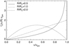 |
Fig. 8 Distribution of ejection speeds (Eq. (4)) for different values of the grain size. |
| In the text | |
|
Fig. 9 Size distribution of freshly ejected salt-rich and salt-poor dust for E5 (at 17.7 km s−1). Yellow areas indicate the size ranges detectable by CDA. These are different for salt-rich and salt-poor dust. Radii |
| In the text | |
|
Fig. 10 Size distribution of freshly ejected salt-rich and salt-poor dust for E17 (at 7.5 km s−1). Yellow areas indicate the size ranges detectable by CDA. These are different for salt-rich and salt-poor dust. Radii |
| In the text | |
|
Fig. 11 Size distribution (arb. normalization) of the E ring particles in the vicinity of Enceladus evaluated from our model as those particles that escape Enceladus. The size distribution of the salt-poor dust grains in the model (at the moment of ejection from the sources on the tiger stripes) as well as a power law R−4.6 are shown for comparison. |
| In the text | |
|
Fig. 12 Number density profile of the E7 flyby recorded by HRD counters M1, m′1, M2, m′2, and M3 and the model fits. The variability factor k = 1 (see Sect. 4.5). |
| In the text | |
|
Fig. 13 Number density profile of the E7 flyby recorded by HRD counters M1, m′1, M2, m′2, and M3 and the model fits. The variability factor k = 1 (see Sect. 4.5). |
| In the text | |
|
Fig. 14 E5 compositional profile measured (symbols) and modeled (lines) comparing the cases with (k = 2) and without (k = 1) and taking into account the plume’s variability. |
| In the text | |
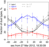 |
Fig. 15 Same as Fig. 14 but for the E17 compositional profile. |
| In the text | |
|
Fig. 16 Density of dust at different altitudes above the SPT of Enceladus. The red cross marks the south pole. The dashed lines denote the ground tracks of hypothetical horizontal flybys (see text). |
| In the text | |
|
Fig. 17 Prediction of our model for the total mass of salt-rich and salt-poor dust collected during hypothetical horizontal flybys (performed along the dashed lines shown in Fig. 16). The mass is calculated for an ideal plane detector of 1 m2 area. Masses for types I and II are added together, giving the salt-poor dust mass. All salt-poor dust particles contain organic compounds, although the actual proportion of mass-spectra showing lines of organics (which classifies them as type II) may depend on the instrument characteristics and flyby velocity. |
| In the text | |
|
Fig. 18 Prediction of our model for the mean radius of salt-rich and salt-poor dust particles encountered on the average along the hypothetical flybys considered in Fig. 17 (dashed lines shown in Fig. 16). |
| In the text | |
|
Fig. 19 Dust-to-gas mass ratio distribution in the plane along the dashed line in Fig. 16 and the center of Enceladus. The light gray area depicts the region that the freshly ejected gas does not reach. The rectangle in panel b marks the region shown in panel a. |
| In the text | |
|
Fig. 20 Salt-rich dust percentage in the same plane as Fig. 19. The proportion has been computed for the whole range of grain sizes used in the model: 0.1–15 µm for both salt-poor and salt-rich dust particles. The rectangle in panel b marks the region shown in panel a. |
| In the text | |
|
Fig. A.1 Number density profiles of the E7 (upper panel) and E21 flybys (lower panel). Comparison of three model setups for the jets: jets 1 — jets from Porco et al. (2014) neglecting tilts; jets 2 — tilted jets from Porco et al. (2014); jets 3 — vertical jets uniformly distributed along the TSs. |
| In the text | |
|
Fig. A.2 E5 compositional profile measured (symbols) and modeled (lines) using the jet sources from Porco et al. (2014). The solid line corresponds to a model that uses the original tilts for the jets as reported in Porco et al. (2014). The dashed line corresponds to a model that neglects these tilts and uses a vertical jet axis instead. |
| In the text | |
|
Fig. A.3 E17 compositional profile measured (symbols) and modeled (lines) using the jet sources from Porco et al. (2014). The solid line corresponds to a model that uses the original tilts for the jets as reported in Porco et al. (2014). The dashed line corresponds to a model that neglects these tilts and uses a vertical jet axis instead. |
| In the text | |
|
Fig. A.4 Number density profiles of the E7 (upper panel) and E21 (lower panel) flybys. Jets from Porco et al. (2014) with more confined ejection than used in the model settings (Eq. (6) with ω = 5°). |
| In the text | |
|
Fig. A.5 Jet with ω = 3°. |
| In the text | |
|
Fig. A.6 Jet with ω = 5°. |
| In the text | |
|
Fig. A.7 Jet with ω = 10°. |
| In the text | |
|
Fig. A.8 E5 compositional profile measured (symbols) and modeled (lines) with a narrow jet ejecting only type II dust with the rate three times higher than the other jets in our model dust added at −81.3° NL 292.8° WL. |
| In the text | |
Current usage metrics show cumulative count of Article Views (full-text article views including HTML views, PDF and ePub downloads, according to the available data) and Abstracts Views on Vision4Press platform.
Data correspond to usage on the plateform after 2015. The current usage metrics is available 48-96 hours after online publication and is updated daily on week days.
Initial download of the metrics may take a while.