| Issue |
A&A
Volume 689, September 2024
|
|
|---|---|---|
| Article Number | A226 | |
| Number of page(s) | 16 | |
| Section | Cosmology (including clusters of galaxies) | |
| DOI | https://doi.org/10.1051/0004-6361/202450219 | |
| Published online | 17 September 2024 | |
Neural network reconstruction of density and velocity fields from the 2MASS Redshift Survey
1
Institute for Theoretical Physics, Heidelberg University,
69120
Heidelberg,
Germany
2
Department of Physics, Technion,
Haifa
3200003,
Israel
e-mail: punyakoti.g@campus.technion.ac.il; adi@physics.technion.ac.il
Received:
2
April
2024
Accepted:
30
May
2024
Aims. Our aim is to reconstruct the 3D matter density and peculiar velocity fields in the local Universe up to a distance of 200 h−1 Mpc from the Two-Micron All-Sky Redshift Survey (2MRS) using a neural network (NN).
Methods. We employed an NN with a U-net autoencoder architecture and a weighted mean squared error loss function trained separately to output either the density or velocity field for a given input grid of galaxy number counts. The NN was trained on mocks derived from the Quijote N-body simulations, incorporating redshift-space distortions (RSDs), galaxy bias, and selection effects closely mimicking the characteristics of 2MRS. The trained NN was benchmarked against a standard Wiener filter (WF) on a validation set of mocks before applying it to 2MRS.
Results. The NN reconstructions effectively approximate the mean posterior estimate of the true density and velocity fields conditioned on the observations. They consistently outperform the WF in terms of reconstruction accuracy and effectively capture the nonlinear relation between velocity and density. The NN-reconstructed bulk flow of the total survey volume exhibits a significant correlation with the true mock bulk flow, demonstrating that the NN is sensitive to information on “super-survey” scales encoded in the RSDs. When applied to 2MRS, the NN successfully recovers the main known clusters, some of which are partially in the Zone of Avoidance. The reconstructed bulk flows in spheres of different radii less than 100 h−1 Mpc are in good agreement with a previous 2MRS analysis that required an additional external bulk flow component inferred from directly observed peculiar velocities. The NN-reconstructed peculiar velocity of the Local Group closely matches the observed Cosmic Microwave Background dipole in amplitude and Galactic latitude, and only deviates by 18° in longitude. The NN-reconstructed fields are publicly available.
Key words: methods: data analysis / methods: numerical / surveys / large-scale structure of Universe
© The Authors 2024
 Open Access article, published by EDP Sciences, under the terms of the Creative Commons Attribution License (https://creativecommons.org/licenses/by/4.0), which permits unrestricted use, distribution, and reproduction in any medium, provided the original work is properly cited.
This article is published in open access under the Subscribe to Open model. Subscribe to A&A to support open access publication.
1 Introduction
The cornerstone of modern cosmology rests on gravity as the driving force behind the formation of the large-scale structure (LSS) observed in the Universe. Initially, minuscule fluctuations, seeded by quantum fluctuations, were magnified through gravitational instability, culminating in the intricate cosmic structures we observe today. The mass density field shaping this cosmic tapestry is predominantly governed by dark matter (DM), which contributes roughly 85% of the mass and thus the gravitational influence, while ordinary baryonic matter constitutes the remaining 15%.
Galaxies trace the underlying density field, congregating in elongated filaments that connect clusters surrounded by vast underdense regions (voids), collectively forming what is known as the cosmic web. Understanding the genesis and evolution of the LSS is paramount for advancing cosmological knowledge and deciphering the Universe’s composition, as well as any deviations from the standard model.
A crucial research objective lies in reconstructing the density and velocity fields from the observed galaxy distribution. The reconstructed galaxy density field offers insights into the large-scale distribution of DM, contingent upon establishing a “biasing relation” that links galaxies to DM. Moreover, within the standard paradigm, a simple relationship exists between peculiar velocity and density, allowing for the inference of the velocity field from the reconstructed density field. This inferred velocity field can then be compared with the observed velocities of galaxies, facilitating the validation of cosmological models and refining our understanding of how galaxies populate DM halos and evolve over cosmic epochs.
More ambitiously, discrepancies between the inferred and observed fields may indicate deviations from standard gravity theory. These deviations could potentially overlap with the biasing relation, making a reliable reconstruction vital for disentangling the consequences of nonstandard gravity from biasing effects. Achieving this requires the development of sophisticated algorithms and techniques capable of accurately mapping density and velocity fields from observational data while rigorously addressing potential biases and uncertainties.
Therefore, substantial effort has been invested in developing reconstruction techniques for inferring cosmological velocity and density fields from observations. The two main types of observational data are (i) catalogs of peculiar velocities of galaxies and (ii) surveys of galaxy redshifts and angular positions on the sky. In this paper we address the latter.
Any reconstruction method of the true mass density from redshift surveys must face the following three main challenges. First, the finite number of observable galaxies introduces shot noise, constituting the primary source of random error. Since only galaxies above a specific flux limit are observed, the dataset is inherently incomplete. To mitigate this issue, each galaxy is weighted by the survey’s selection function. This adjustment compensates for the survey’s incompleteness at varying distances, enabling a more precise statistical analysis of the galaxy distribution.
Second, galaxies reside within DM halos, and their properties and distribution are influenced by the complex accretion and merging history of these halos. Consequently, the biasing relation between the observed galaxy distribution and the underlying DM density field is complex and nonlinear. Establishing a model for this biasing relation is crucial for any attempt to accurately reconstruct the DM density field from the observed distribution of galaxies.
Third, a galaxy’s redshift is affected by its peculiar velocity, in addition to the Hubble expansion velocity. This leads to anisotropies in the galaxy distribution as observed in redshift space rather than real-distance space. These redshift-space distortions (RSDs) introduce systematic deviations from the true galaxy distribution. Correcting for these distortions is crucial to accurately infer the underlying mass density field. On large scales (larger than a few megaparsec), the peculiar velocity field is coherent with the underlying density and hence causes an enhancement of density fluctuations relative to real space. This anisotropic enhancement can actually be used to constrain cosmological parameters. On small scales, random galaxy motions stretch their apparent distribution along the line of sight in redshift space, creating elongated structures known as “Fingers of God” (Jackson 1972; Sargent & Turner 1977; Tully & Fisher 1978). Both coherent flows and random motions need to be properly addressed in any successful reconstruction.
Prior to the significant growth and widespread adoption of machine learning in various fields, including cosmology, traditional methods for analyzing LSS observations primarily relied on specific assumptions that could be formulated either analytically or numerically in a compact, well-defined manner. The reconstruction of velocity fields from redshift surveys, for example, required specific density-velocity correlations derived from approximate dynamics. Such correlations were based on models found in linear theory (e.g. Peebles 1980) or quasi-linear approaches, such as the Zel’dovich approximation (Zel’dovich 1970; Nusser et al. 1991), 2LPT (Moutarde et al. 1991; Bouchet et al. 1992, 1995; Buchert & Ehlers 1993; Gramann 1993; Zheligovsky & Frisch 2014), and the least action principle (Peebles 1989; Nusser & Branchini 2000).
To mitigate the effect of shot noise, most reconstruction methods employ a smoothing of the discrete galaxy distribution with an extended (e.g. Gaussian) kernel to obtain a galaxy density field (e.g. Yahil et al. 1991; Carrick et al. 2015; Boruah et al. 2020). Another popular technique is applying a Wiener filter (WF) (Wiener 1949), which yields the linear minimum variance estimator of the true density / velocity fields given the observed data (e.g. Zaroubi et al. 1995; Fisher et al. 1995; Webster et al. 1997; Schmoldt et al. 1999; Erdoğdu et al. 2006; Lilow & Nusser 2021). For the special case of Gaussian data and true fields, the WF coincides with the mean and maximum of the posterior distribution of the true fields given the data. A different approach to relate the distributions of noisy, biased tracers and the underlying matter field is based on optimal transport theory (Brenier et al. 2003; Nikakhtar et al. 2023, 2024). Another widely used class of reconstruction methods are hierarchical Bayesian models (e.g. Jasche & Lavaux 2019; Kitaura et al. 2021), which draw samples from a posterior distribution that combines different models for gravitational dynamics, RSDs, and biasing relations in a forward-modelling approach. This approach allows for the description of nonlinear relations and non-Gaussian statistics but is usually computationally expensive and still relies on explicit (approximate) modelling assumptions.
The primary advantage of neural networks (NNs) over traditional approaches lies in their ability to infer the relationship between the underlying true fields and the observed LSS data without predefining the functional form of this relationship. Thus, NN algorithms particularly excel at processing training data encompassing a broad spectrum of physical effects. These effects are often too complex for analytical models to accurately capture or computationally too expensive to be evaluated numerically during the inference process. Recent years have therefore seen a rise in studies where NNs are trained to reconstruct density and velocity fields from observations (e.g. Wu et al. 2021; Shallue & Eisenstein 2023; Ganeshaiah Veena et al. 2023; Qin et al. 2023; Chen et al. 2023; Wu et al. 2023; Legin et al. 2024; Chen et al. 2024).
In a previous paper, Ganeshaiah Veena et al. (2023, hereafter Paper I), we have assessed the applicability of an NN for the reconstruction of 3D matter density and velocity fields from a sample of observed galaxies. For that purpose, a simplified set of training data was used, employing 2LPT dynamics, imposing RSDs along the z- rather than radial direction, and not including any galaxy biasing or survey selection effects. This proof-of-concept demonstrated that an NN is capable of efficiently learning to evaluate the non-Gaussian mean posterior estimate of the true fields given the observations, yielding a consistently better reconstruction accuracy than a reference WF.
In the current paper, our objective is to apply this NN framework to the Two-Micron All-Sky Redshift Survey (2MRS) (Huchra et al. 2012; Macri et al. 2019) in order to obtain high-quality reconstructions of the 3D matter density and velocity fields in the local Universe. To achieve this, we used the highresolution N-body simulations of the Quijote suite (Villaescusa-Navarro et al. 2020) to extract training data that incorporate accurate gravitational dynamics and mimic the survey characteristics of 2MRS as closely as possible.
The structure of the paper is as follows. In Sect. 2, we provide a brief overview of 2MRS, concentrating on its key properties relevant to the generation of mock data. Additionally, this section introduces the Quijote simulations and describes their use in creating mock data that emulate the characteristics of the actual 2MRS. The generated mock data are intended for the training of our NN, detailed in Sec. 3. Comprehensive testing of the NN, utilizing a validation set of mock data, is documented in Sec. 4. The outcomes of applying the NN to the actual 2MRS data are presented and examined in Sec. 5. The paper concludes with Sec. 6, offering a summary and discussion of the findings.
2 Data
2.1 2MRS
The 2MRS is a flux-limited survey with a Ks-band magnitude of Ks ≤ 11.75, providing sky positions and spectroscopic redshifts for 44, 572 galaxies (Huchra et al. 2012; Macri et al. 2019). Its footprint covers 91% of the sky, only missing a thin band covered by the Milky Way, the so-called Zone of Avoidance (ZoA).
In our reconstruction, we consider a spherical volume with a radius of rmax = 200 h−1 Mpc, encompassing 98% of the 2MRS galaxies. Outside of the ZoA, the observable fraction of galaxies follows a selection function ϕ(r) that solely depends on the distance from the observer. To robustly estimate ϕ(r), we adopt the methodology outlined in Lilow & Nusser (2021). This involves imposing a partial volume limit at a distance of 30 h−1 Mpc and utilizing an F/T-estimator (Davis & Huchra 1982; Branchini et al. 2012). The number of galaxies within rmax satisfying the partial volume limit is Ng = 42 648. However, unlike Lilow & Nusser (2021), we directly employ individual observed galaxy redshifts in the Cosmic Microwave Background (CMB) frame rather than redshifts associated with galaxy groups. While grouping galaxies is typically undertaken to mitigate Fingers-of-God effects in redshift space, we found it unnecessary for generating high-quality NN reconstructions.
The selection-function-corrected mean galaxy number density within the reconstruction volume is given by
![$\[\bar{n}^{\mathrm{g}}=\frac{3}{4 \pi r_{\text {max }}^3 F_{\text {sky }}} \sum_{a=1}^{N^g} \frac{1}{\phi\left(s_a\right)} \approx 1.83 \times 10^{-2} h^3 ~\mathrm{Mpc}^{-3},\]$](/articles/aa/full_html/2024/09/aa50219-24/aa50219-24-eq1.png) (1)
(1)
where Fsky ≈ 0.91 is the fraction of the sky not obscured by the ZoA, and ϕ(sa) is evaluated at the comoving redshift-space distances sa of the observed galaxies.
The 2MRS galaxy number count field used as input to the NN reconstruction was obtained by defining a regular 128 × 128 × 128 cubic grid of 400 h−1 Mpc side length enclosing the reconstruction volume and assigning each of the Ng galaxies to the grid point nearest to the galaxy’s redshift-space coordinate sa.
2.2 Mock data
The accuracy of an NN reconstruction hinges upon the quality of the training data it receives. To generate mocks that employ an accurate model of nonlinear DM dynamics on scales ≳ 3 h−1 Mpc, we used the Quijote N-body simulations suite, which aims at providing a sufficiently large number of high-quality simulations for training machine learning applications (Villaescusa-Navarro et al. 2020). For this paper, we used the 100 high-resolution fiducial cosmology runs, each containing 10243 equal-mass particles in a cubic box with side length 1000 h−1 Mpc. The cosmological parameters used are Ωm = 0.3175, Ωb = 0.049, h = 0.6711, ns = 0.9624, σ8 = 0.834, which are in good agreement with the Planck 2018 constraints (Planck Collaboration VI 2020b).
From every simulation box we extracted 64 partially overlapping cubic sub-boxes of side length 400 h−1 Mpc, resulting in a total number of 6400 mocks. Among these, 5760 were designated for training data, while the remaining 640 were set aside for validation purposes. Although neighboring mocks are not completely independent, as they overlap by 150 h−1 Mpc, we found this to result in a better NN training convergence than using fewer nonoverlapping mocks. In part, this is due to the independently created mock observations, as described in the following.
To ensure that the mock observations are as close as possible to the actual 2MRS characteristics, we accounted for RSDs, ZoA, selection function ϕ(r) and galaxy bias. Due to the flux-limit of 2MRS, the minimum luminosity of observable galaxies increases with distance, leading to a radially growing galaxy bias. To reproduce this in our mocks, we assumed that a galaxy can only form in regions where the matter density 1 + δ is above a radially increasing threshold ρth(r). The expected number of formed galaxies is then proportional to the modified density
![$\[1+\delta^{\text {th }}(\boldsymbol{r})= \begin{cases}(1+\delta(\boldsymbol{r})) \mathcal{N}(r) & \text { if } 1+\delta(\boldsymbol{r}) \geq \rho^{\text {th }}(r), \\ 0 & \text { else },\end{cases}\]$](/articles/aa/full_html/2024/09/aa50219-24/aa50219-24-eq2.png) (2)
(2)
where the normalization factor ![$\[\mathcal{N}(r)\]$](/articles/aa/full_html/2024/09/aa50219-24/aa50219-24-eq3.png) was chosen such that the ensemble average of 1 + δth(r) at any position r is unity. The threshold values ρth(r) for different radii were calibrated such that the resulting galaxy density fluctuation amplitude
was chosen such that the ensemble average of 1 + δth(r) at any position r is unity. The threshold values ρth(r) for different radii were calibrated such that the resulting galaxy density fluctuation amplitude ![$\[\sigma_8^{\mathrm{g}}(r)\]$](/articles/aa/full_html/2024/09/aa50219-24/aa50219-24-eq4.png) in our mocks matches that of 2MRS (computed using the method described in Appendix A of Lilow & Nusser 2021).
in our mocks matches that of 2MRS (computed using the method described in Appendix A of Lilow & Nusser 2021).
The mock matter density and peculiar velocity fields, used as NN targets, and the mock galaxy number count fields, used as NN inputs, were then obtained as follows: (i) In each sub-box, the mean simulation particle density as well as the mean and variance of the particle velocities were computed on a regular 128 × 128 × 128 grid, using a Cloud-in-Cell (CIC) assignment scheme. The mean particle density and velocity grids constituted the mock matter density and peculiar velocity fields, respectively. (ii) For each grid cell j at a distance rj ≤ rmax to the sub-box center, a random number Nj of observed galaxies was drawn from a Poisson distribution ![$\[\operatorname{Pois}\left(N_j \mid \bar{N}_j\right)\]$](/articles/aa/full_html/2024/09/aa50219-24/aa50219-24-eq5.png) around the expected number of observable galaxies in that cell,
around the expected number of observable galaxies in that cell, ![$\[\bar{N}_j=\left(1+\delta_j^{\mathrm{th}}\right) \phi\left(r_j\right) \bar{n}^{\mathrm{g}} ~V\]$](/articles/aa/full_html/2024/09/aa50219-24/aa50219-24-eq6.png) . Here,
. Here, ![$\[1+\delta_j^{\mathrm{th}}\]$](/articles/aa/full_html/2024/09/aa50219-24/aa50219-24-eq7.png) is the grid cell’s modified matter density according to Eq. (2),
is the grid cell’s modified matter density according to Eq. (2), ![$\[\bar{n}^{\mathrm{g}}\]$](/articles/aa/full_html/2024/09/aa50219-24/aa50219-24-eq8.png) is the selection-function-corrected mean 2MRS galaxy number density Eq. (1) and V is the volume of a grid cell. (iii) The real-space Galactic coordinates of the Nj galaxies were each set to an independent uniformly random position ra within the grid cell j. If ra = 0 or if the galaxy’s Galactic longitude and latitude lie within the ZoA, this galaxy was discarded. (iv) Each remaining galaxy was assigned a peculiar velocity va drawn from a Gaussian distribution whose mean and variance are the CIC-assigned mean and variance of the simulation particle velocities, linearly interpolated between grid points at the galaxy position ra. (v) The observed galaxy red-shift was given by
is the selection-function-corrected mean 2MRS galaxy number density Eq. (1) and V is the volume of a grid cell. (iii) The real-space Galactic coordinates of the Nj galaxies were each set to an independent uniformly random position ra within the grid cell j. If ra = 0 or if the galaxy’s Galactic longitude and latitude lie within the ZoA, this galaxy was discarded. (iv) Each remaining galaxy was assigned a peculiar velocity va drawn from a Gaussian distribution whose mean and variance are the CIC-assigned mean and variance of the simulation particle velocities, linearly interpolated between grid points at the galaxy position ra. (v) The observed galaxy red-shift was given by ![$\[1+z_a^{\text {obs }}=\left(1+z_a\right)\left(1+\frac{\boldsymbol{v}_a {\cdot} \boldsymbol{r}_a}{c ~r_a}\right)\]$](/articles/aa/full_html/2024/09/aa50219-24/aa50219-24-eq9.png) , where za is the cosmological redshift corresponding to the galaxy’s comoving distance, ra = Dcom(za), and c is the speed of light. If
, where za is the cosmological redshift corresponding to the galaxy’s comoving distance, ra = Dcom(za), and c is the speed of light. If ![$\[z_a^{\text {obs }}<0\]$](/articles/aa/full_html/2024/09/aa50219-24/aa50219-24-eq10.png) , this galaxy was discarded. Otherwise, the galaxy’s redshift-space coordinate was
, this galaxy was discarded. Otherwise, the galaxy’s redshift-space coordinate was ![$\[\boldsymbol{s}_a=D_{\mathrm{com}}\left(z_a^{\mathrm{obs}}\right) \frac{\boldsymbol{r}_a}{r_a}\]$](/articles/aa/full_html/2024/09/aa50219-24/aa50219-24-eq11.png) . (vi) Finally, the mock galaxy number count field Nobs was obtained by assigning each remaining galaxy to the grid point nearest to the galaxy’s redshift-space coordinate sa.
. (vi) Finally, the mock galaxy number count field Nobs was obtained by assigning each remaining galaxy to the grid point nearest to the galaxy’s redshift-space coordinate sa.
3 Neural network
An NN is a computational model with adjustable weights and biases, fine-tuned by minimizing a loss function, to predict targets from input data. It consists of layers, each with multiple neurons, where weights adjust connection strengths and biases set activation thresholds.
Our main goal is to train an NN to infer the 3D matter density and peculiar velocity fields from noisy observed galaxy number counts, described in detail in Sec. 2. For this purpose, we trained two separate NNs: one for the density field and another for the velocity field.
We utilized an autoencoder with U-Net architecture, which has proven effective for this reconstruction task in Paper I. It comprises an encoder, which compresses the input to a lower-dimensional latent space representation, and a decoder, which reconstructs the target from the latent space representation. Both input and target fields were represented as 128 × 128 × 128 grids, and the latent space dimension was (8 × 8 × 8)grids × 128filters. In summary, the encoder used a series of 3D convolution steps with ReLU activation and max pooling to reduce the grid size; the decoder employed a symmetric series of 3D transpose convolution steps with ReLU activation to expand the grid size again. Skip connections between the encoder and decoder helped maintain the spatial feature localization and improve the training convergence. The density NN included a final ReLU activation, ensuring that no negative densities are generated, whereas the velocity NN used a linear final activation. The precise NN architecture, including the numbers of convolutional filters, is detailed in Paper I. The only modification made in the present work was to reduce the depth of the NN by one step (in Paper I the latent dimension was (4 × 4 × 4)grids × 256filters), resulting in a total number of ~1.6 × 10⁶ trainable parameters. This change was found to reduce overfitting without sacrificing reconstruction accuracy.
Before being fed into the NN, the input data underwent preprocessing to ensure that the values are predominantly constrained within the range of 0–1. The input galaxy number counts and the target density fields were both divided by a factor of 40, while the target velocity fields were divided by 300, approximately matching the standard deviation per velocity component.
As discussed in Paper I, the choice of loss function determines the type of statistical estimator learned by the NN. Specifically, we are interested in computing the mean posterior estimate ![$\[\hat{T}_j \in\left\{\hat{\delta}_j^{\mathrm{NN}}, \hat{\boldsymbol{v}}_j^{\mathrm{NN}}\right\}\]$](/articles/aa/full_html/2024/09/aa50219-24/aa50219-24-eq12.png) of the target fields
of the target fields ![$\[T_j \in\left\{\delta_j^{\text {true }}, \boldsymbol{v}_j^{\text {true}}\right\}\]$](/articles/aa/full_html/2024/09/aa50219-24/aa50219-24-eq13.png) given an input field
given an input field ![$\[I_j=N_j^{\text {obs }}\]$](/articles/aa/full_html/2024/09/aa50219-24/aa50219-24-eq14.png) , where j = 1, . . ., Mgrid labels the individual grid cells. This is achieved by employing a (weighted) mean squared error loss function,
, where j = 1, . . ., Mgrid labels the individual grid cells. This is achieved by employing a (weighted) mean squared error loss function,
![$\[\begin{aligned}&\operatorname{Loss}(\hat{T})=\underbrace{\sum_{I, T} P(I, T)}_{\sum_I P(I) \sum_T P(T/I)} \sum_{j=1}^{\sum_{\text {grid }}} \omega_j\left(T_j-\hat{T}_j(I)\right)^2,\\\end{aligned}\]$](/articles/aa/full_html/2024/09/aa50219-24/aa50219-24-eq15.png) (3)
(3)
where ωj is a grid-cell-dependent weighting factor and P(I, T) is the joint probability distribution of input and target fields. Via Bayes’ theorem, the latter can be split into the evidence P(I) and the posterior P(T|I). Minimizing this loss function yields
![$\[0=\frac{\delta \operatorname{Loss}(\hat{T})}{\delta \hat{T}_j(I)}=-2 ~\omega_j ~P(I) ~\sum_T P(T \mid I)\left(T_j-\hat{T}_j(I)\right)\]$](/articles/aa/full_html/2024/09/aa50219-24/aa50219-24-eq16.png) (4)
(4)
and thus the desired mean posterior estimate
![$\[\hat{T}_j(I)=\sum_T ~P(T \mid I) T_j=\left\langle T_j \mid I\right\rangle.\]$](/articles/aa/full_html/2024/09/aa50219-24/aa50219-24-eq17.png) (5)
(5)
Formally, any ![$\[\hat{T}\]$](/articles/aa/full_html/2024/09/aa50219-24/aa50219-24-eq18.png) -independent choice of the weighting factor ωj results in the same estimator1. But since during training the loss function is minimized numerically via stochastic gradient descent (Goodfellow et al. 2016), the choice of weighting can influence the numerical convergence and thus the actually learned estimator. Also, we note that in practice the infinite sum over all possible samples from P(I, T) in Eq. (4) needs to be approximated by a sum over a finite set of training samples.
-independent choice of the weighting factor ωj results in the same estimator1. But since during training the loss function is minimized numerically via stochastic gradient descent (Goodfellow et al. 2016), the choice of weighting can influence the numerical convergence and thus the actually learned estimator. Also, we note that in practice the infinite sum over all possible samples from P(I, T) in Eq. (4) needs to be approximated by a sum over a finite set of training samples.
For the training of the density reconstruction NN, we found that a weighting with the survey selection function, ωj ∞ ϕ(rj), improves the training convergence. This choice was motivated by the fact that ϕ is proportional to the inverse variance of the observed galaxy shot noise. We hence minimized the loss function
![$\[\operatorname{Loss}\left(\hat{\delta}^{\mathrm{NN}}\right)=\frac{1}{M_{\text {train }} M_{\text {grid }}} \sum_{\alpha=1}^{M_{\text {train }}} \sum_{j=1}^{M_{\text {grid }}} \phi\left(r_j\right)\left(\delta_j^{\text {true }, \alpha}-\hat{\delta}_j^{\mathrm{NN}, \alpha}\right)^2,\]$](/articles/aa/full_html/2024/09/aa50219-24/aa50219-24-eq19.png) (6)
(6)
where α = 1,..., Mtrain labels the individual mock realizations used for training.
For the training of the velocity reconstruction NN, one could use an equivalent loss function for the individual velocity components, but that would require an NN with three output channels or three separate NNs, since the ZoA (which has different widths for different Galactic latitudes) breaks the symmetry between the velocity components. However, this can potentially result in the prediction of a spurious rotational component in the reconstructed velocity field, which we know to be absent on the scales ≳3 h−1 Mpc probed in our setup2.
Therefore, we instead imposed the reconstruction of an irrotational velocity field by assuming a potential flow, ![$\[\hat{\boldsymbol{v}}^{\mathrm{NN}}=\boldsymbol{\nabla} \hat{\Psi}^{\mathrm{NN}}\]$](/articles/aa/full_html/2024/09/aa50219-24/aa50219-24-eq20.png) , and training the NN to reconstruct the velocity potential
, and training the NN to reconstruct the velocity potential ![$\[\hat{\Psi}^\text{NN}\]$](/articles/aa/full_html/2024/09/aa50219-24/aa50219-24-eq21.png) . This also improved the training convergence compared to learning to reconstruct the individual velocity components directly. Beyond that, the convergence was empirically found to be further improved by using a weighting ωj ∝ ϕ(rj)/rj, which gives even more weight to grid cells at smaller distances than the weighting in the density loss function. The velocity (potential) loss function thus reads
. This also improved the training convergence compared to learning to reconstruct the individual velocity components directly. Beyond that, the convergence was empirically found to be further improved by using a weighting ωj ∝ ϕ(rj)/rj, which gives even more weight to grid cells at smaller distances than the weighting in the density loss function. The velocity (potential) loss function thus reads
![$\[\operatorname{Loss}\left(\hat{\Psi}^{\mathrm{NN}}\right)=\frac{1}{M_{\text {train }} M_{\text {grid }}} \sum_{\alpha=1}^{M_{\text {train }}} \sum_{j=1}^{M_{\text {grid }}} \frac{\phi\left(r_j\right)}{r_j}\left(\boldsymbol{v}_j^{\text {true }, \alpha}-\boldsymbol\nabla \hat{\Psi}_j^{\mathrm{NN}, \alpha}\right)^2,\]$](/articles/aa/full_html/2024/09/aa50219-24/aa50219-24-eq22.png) (7)
(7)
where the potential gradient is computed via symmetric finite differences.
The NNs were implemented in Keras (Chollet et al. 2015) with a TensorFlow backend (Abadi et al. 2016). Using the AMS-Grad variant of the Adam parameter optimizer (Kingma & Ba 2017; Reddi et al. 2019) with learning rate 10−4 and a batch size of 4 mock realizations per gradient update, training the density and velocity (potential) reconstruction NNs for 100 epochs took around 12 hours each on an NVIDIA 3090 GPU. Once trained, the NN reconstruction of either target field for a given galaxy number count field takes just a fraction of a second.
The loss functions as a function of the training epoch, evaluated for both the training and the validation set are shown in Fig. 1. For the density (left panel), the training loss drops quickly at first before settling into a slow and steady decrease after ~20 epochs. The validation loss initially follows the training loss, then plateaus after ~40 epochs, fluctuates around its minimum for some time and eventually starts to weakly increase again after ~80 epochs. For the velocity (right panel), a qualitatively similar behavior is seen, but with a faster initial drop in training loss, followed by a much slower steady decrease after ~10 epochs. The velocity validation loss stabilizes after ~40 epochs, showing only minor fluctuations but no sign of increasing again within the 100 epochs. For the reconstructions in the subsequent sections we employ the NN models at the epochs with the minimal validation loss, epoch 75 for the density and epoch 60 for the velocity.
4 Validating the reconstruction using the mocks
In the following, we assess the reconstruction quality achieved by the trained NN by performing a number of tests on the validation set of 640 mocks, described in Sec. 2.2. For some of those tests, we compare the NN results against the widely used and robust WF, serving as a benchmark. We specifically employ the WF implementation presented in Lilow & Nusser (2021), which is designed for all-sky surveys such as 2MRS. It combines the WF with a linear RSD correction, and exploits the isotropy of the survey by expanding the WF in spherical Bessel functions and spherical harmonics (Fisher et al. 1995). This requires filling up the ZoA by copying galaxies from adjacent regions (Yahil et al. 1991), which only has a minor impact on the WF reconstruction results outside of the ZoA, though, as the ZoA only blocks a small portion of the sky.
For all tests, the reconstructed as well as true density and velocity fields were first smoothed using a Gaussian window of width rsmooth = 3 h−1 Mpc, approximately matching the spatial resolution of the employed field grids, to reduce aliasing effects.
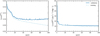 |
Fig. 1 Loss functions as a function of training epochs. Left panel: loss function of the reconstructed density field, given in Eq. (6), in the validation (solid blue) and training (dashed light blue) sets of mocks. Right panel: same for the peculiar velocity potential field, given in Eq. (7). |
4.1 Visual inspection
In Fig. 2, we present the observed, true and NN-reconstructed fields for a single example mock, chosen for its qualitative similarity to the distribution of structures seen in 2MRS. We are showcasing the fields both in a slice through the mock Supergalactic plane (SGP, left panels) and the mock Galactic plane (GP, right panels). The field values on those slices were obtained by linear interpolation between the grid values, resulting in an effective slice thickness of ~3 h−1 Mpc, approximately matching the grid resolution.
For the density in the SGP, the visual inspection reveals a good agreement between the true and reconstructed fields. Large-scale structures, particularly those near the center where galaxies sample the matter distribution densely, are robustly reconstructed. Dense regions are faithfully reproduced, and the larger filamentary structures within the slice are also captured in the reconstruction. Even in the more sparsely sampled outer regions, the NN effectively reconstructs structures to a significant extent.
However, we note a slight discrepancy in the representation of underdense regions, such as voids. They appear slightly less underdense in the reconstructed fields compared to the true fields. This discrepancy is attributed to the NN-reconstructed fields representing the mean of all possible true realizations (mean posterior estimate) and has already been seen and discussed in Paper I.
In the GP, which cuts directly through the ZoA, the top-right panel only reveals a few galaxies near the center, where the ~3 h−1 Mpc thick slice extends beyond the ZoA (which spans a fixed range in latitudes rather than a fixed distance perpendicular to the GP). Despite the diminished number of tracers, the reconstruction in the GP (bottom-right panel) effectively captures the most dominant structures on large scales, even at considerable distances from the observer. Particularly, the large filamentary structure seen in the top-left quadrant of the true field (middle-right panel) is well-captured in the reconstructed field (the bottom-right panel). Naturally, though, the reconstruction is generally more successful at distances closer to the observer where the width of the ZoA is smaller.
The velocity fields are overlaid in Fig. 2 as arrows. The coherence between density and velocity is apparent in all relevant panels, as expected by the gravitational instability theory for structure formation. It effectively captures the overall convergence in regions of higher density and divergence in regions of lower density. The velocity flow seen in the reconstructed fields is remarkably close to the flows in the true fields, especially in the SGP. But even in the sparsely sampled GP, the true and reconstructed velocity fields show a good agreement in all but a few, typically outer regions. This higher reconstruction accuracy of the velocity field compared to the density field in the GP is expected to be a consequence of the significantly larger correlation length of the density field, which allows the ZoA to be partially bridged.
4.2 RMS and RMSE versus distance
For a more quantitative assessment of the reconstructions, we computed the root mean square (RMS) of the reconstructed fields and the root mean squared error (RMSE) between the reconstructed and true fields. In Fig. 3 we show these quantities, averaged across all validation mocks, for both the density and velocity fields as a function of the distance from the observer at r = 0. Both the RMS and RMSE values were computed in spherical shells, each spanning 10 h−1 Mpc in width and extending out to a distance of 200 h−1 Mpc.
For r ≲ 100 h−1 Mpc, the RMS of the NN-reconstructed density (blue curve in top-left panel) is impressively close to the RMS value obtained from the true density fields (dotted horizontal line). At larger radii, the RMS becomes significantly lower than the true value, due to the reduced number density of galaxies at these distances. Since the NN-reconstructed density approximates the mean of all true fields consistent with the observations, its RMS is expected to lie below the true value.
Although the performance of the WF (orange curve) matches that of the NN at large distances, it is clearly less successful at consistently approximating the true value for smaller distances. In fact, it even overshoots the true value close to the center by about 30%.
A similar behavior is observed for the RMS of the radial and tangential velocity components (top-right panel). At r ≲ 100 h−1 Mpc, the NN successfully recovers the RMS for both components with high accuracy. The radial component (solid blue curve) nearly converges exactly to the RMS of the true velocity field components (dotted line), while the tangential component (dashed blue curve), falls only slightly short of reaching the true RMS.
The bottom panels in Fig. 3 plot curves of the RMSE versus distance. Here, lower RMSE values indicate a closer match between the reconstructed fields and the true ones.
For the density (bottom-left panel), the RMSE is lowest at r ≈ 25 h−1 Mpc and then gradually increases toward the boundary of the reconstruction volume at r = 200 h−1 Mpc. Overall, the NN estimates consistently exhibits a lower RMSE than the corresponding WF estimates.
At r ≲ 25 h−1 Mpc, the RMSE increases as we approach the origin. This increase arises primarily due to RSD effects, since the peculiar velocity at the origin induces an artificial dipole enhancement of the density in redshift space. We confirmed that the discrepancy does not exist when the NN is trained on real-space mock observations or when the reconstructed field is smoothed over larger smoothing scales.
The velocity estimates (bottom-right panel) also exhibit a similar trend: low RMSE values at small distances that gradually increase toward the boundary, both for the radial and tangential components. The NN estimates consistently exhibit closer agreement with the true values compared to the WF estimates.
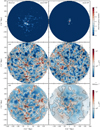 |
Fig. 2 Observed, true and reconstructed fields in a slice through the Supergalactic (left) and Galactic (right) planes for one of the validation mocks. Top row: observed galaxy numbers. The red cross marks the position of the observer at the origin. Middle row: true density (heat map and contours) and peculiar velocity (arrows) fields. The values represented by the contours are marked in the color bar. A reference arrow representing a velocity of 500 km s−1 is shown on the right. Bottom row: corresponding NN-reconstructed fields. |
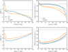 |
Fig. 3 Root mean square (top) and root mean squared error (bottom) of the reconstructed fields as a function of distance. Top-left panel: root mean square of the reconstructed density contrast for the NN (blue) and WF (orange) in the validation mocks. The RMS is averaged over spherical shells of width 10 h−1 Mpc. For reference, the RMS of the true field is marked by the horizontal dotted line. Top-right panel: same for the radial (solid) and tangential (dashed) peculiar velocity components. Bottom row: same for the root mean squared error. |
4.3 Distribution of true versus reconstructed field values
We highlight the differences between the true and reconstructed field values through a detailed point-by-point comparison in Fig. 4, presented as iso-density contours of the distribution of true versus reconstructed values. The contours encompass different fractions of the grid points within the reconstruction volume, as indicated in the figure, revealing detailed characteristics of the distribution.
For the density (left panel), we clearly see that the NN contours (blue) are generally tighter than the WF contours (orange), thus describing a smaller scatter between true and reconstructed densities. Most notably, the contours for the WF extend toward far smaller reconstructed densities than found for the true density, 1 + δtrue ≳ 0.05. In fact, although not visible in this log-plot, the WF-reconstructed densities, ![$\[1+\hat{\delta}^{\mathrm{WF}}\]$](/articles/aa/full_html/2024/09/aa50219-24/aa50219-24-eq23.png) , sometimes even reach negative values, as the linear WF estimator does not guarantee the positivity of the density. In contrast, the NN-reconstructed densities are constrained to
, sometimes even reach negative values, as the linear WF estimator does not guarantee the positivity of the density. In contrast, the NN-reconstructed densities are constrained to ![$\[1+\hat{\delta}^{\mathrm{NN}} ~\gtrsim ~0.2\]$](/articles/aa/full_html/2024/09/aa50219-24/aa50219-24-eq24.png) . This matches the observation from the visual field inspection in Sect. 4.1 that the NN slightly overpredicts the density in very underdense regions, explained by the properties of the mean posterior estimate.
. This matches the observation from the visual field inspection in Sect. 4.1 that the NN slightly overpredicts the density in very underdense regions, explained by the properties of the mean posterior estimate.
If the NN-reconstructed density contrast ![$\[\hat{\delta}^{\mathrm{NN}}\]$](/articles/aa/full_html/2024/09/aa50219-24/aa50219-24-eq25.png) approaches the mean posterior, in accordance with Eq. (5), then it is expected that the conditional mean of δtrue given
approaches the mean posterior, in accordance with Eq. (5), then it is expected that the conditional mean of δtrue given ![$\[\hat{\delta}^{\mathrm{NN}}\]$](/articles/aa/full_html/2024/09/aa50219-24/aa50219-24-eq26.png) will converge to
will converge to
![$\[\left\langle\delta^{\text {true }} \mid \hat{\delta}^{\mathrm{NN}}\right\rangle=\hat{\delta}^{\mathrm{NN}},\]$](/articles/aa/full_html/2024/09/aa50219-24/aa50219-24-eq27.png) (8)
(8)
and the analogous behavior is expected for the velocity. The solid blue line shows the conditional mean computed from the actual fields by averaging the values of δtrue in different bins of ![$\[\hat{\delta}^{\mathrm{NN}}\]$](/articles/aa/full_html/2024/09/aa50219-24/aa50219-24-eq28.png) . The result matches the diagonal dotted one-to-one line with almost perfect agreement. The only notable deviation is the smallest bin around 1 +
. The result matches the diagonal dotted one-to-one line with almost perfect agreement. The only notable deviation is the smallest bin around 1 + ![$\[\hat{\delta}^{\mathrm{NN}}\]$](/articles/aa/full_html/2024/09/aa50219-24/aa50219-24-eq29.png) = 0.2. However, it can be seen from the contours that this bin encompasses only a tiny fraction of less than 1% of all points. By comparison, the conditional average of true given WF-reconstructed densities (solid orange line) deviates significantly from the diagonal line for any underdense values and also shows notable discrepancies for overdensities. This is expected because the WF should only reproduce the mean posterior estimate accurately if both the true and observed fields were Gaussian.
= 0.2. However, it can be seen from the contours that this bin encompasses only a tiny fraction of less than 1% of all points. By comparison, the conditional average of true given WF-reconstructed densities (solid orange line) deviates significantly from the diagonal line for any underdense values and also shows notable discrepancies for overdensities. This is expected because the WF should only reproduce the mean posterior estimate accurately if both the true and observed fields were Gaussian.
The error bars attached to the solid lines mark the range of the most likely 68% true densities given a reconstructed density value. These error bars are asymmetrical around the conditional true mean values, reflecting the asymmetry of the underlying conditional distribution, as discussed in more detail in Sect. 4.4. We see that the error bars for the NN are consistently narrower than those for the WF, especially at the low and high density tails, demonstrating the superior predictive power of the NN.
It is important to note that while Eq. (8) holds at least approximately, this is not true for the analogous relation for the reversed conditional mean, ![$\[\left\langle\hat{\delta}^{\mathrm{NN}} \mid \delta^{\text {true }}\right\rangle \neq \delta^{\text {true }}\]$](/articles/aa/full_html/2024/09/aa50219-24/aa50219-24-eq30.png) . That is, the mean posterior estimate is biased in the sense that the conditional average of reconstructed values for a given true value does generally not match that true value. This is demonstrated by the dashed blue line (to be understood as a function of δtrue), which strongly deviates from the diagonal line. The same is true for the WF (dashed orange line).
. That is, the mean posterior estimate is biased in the sense that the conditional average of reconstructed values for a given true value does generally not match that true value. This is demonstrated by the dashed blue line (to be understood as a function of δtrue), which strongly deviates from the diagonal line. The same is true for the WF (dashed orange line).
We find a similar trend for the peculiar velocity reconstructions in the right panel of Fig. 4. The contours are tighter for the NN compared to the WF fields. The conditional mean of true given reconstructed velocities (solid lines) closely follows the one-to-one line for the NN, but notably deviates from it for the WF, in particular for reconstructed velocity components beyond ±700 km s−1 as well as close to the true velocity component RMS of approximately ±270 km s−1. Furthermore, the range of the 68% most likely true velocity values given a reconstructed value is consistently tighter for the NN than for the WF. Lastly, like for the density, the conditional mean of reconstructed given true velocities (dashed lines) significantly deviates from the one-to-one line.
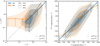 |
Fig. 4 Distribution of true versus reconstructed field values. Left panel: distribution of true versus reconstructed density values for the NN (blue) and WF (orange) reconstructions in the validation mocks, represented as shaded areas bounded by the iso-density contours of the distribution. Going from a darker to lighter hue, the shaded areas contain 50, 90, and 99% of all the points, respectively. The conditional mean true values and the 68% most likely true values for a given reconstructed value are shown as solid lines and error bars, respectively. The average reconstructed values for a given true value are shown as dashed lines (understood as a function of the true values). For reference, the diagonal is marked with a dotted line. Right panel: same for the peculiar velocity components. |
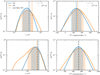 |
Fig. 5 Conditional distributions of true given reconstructed field values. Top-left panel: conditional distribution of true densities for a given reconstructed density |
![$\[1+\hat{\delta}=0.36\]$](/articles/aa/full_html/2024/09/aa50219-24/aa50219-24-eq31.png)
![$\[\hat{\boldsymbol{v}}=267 \mathrm{~km} \mathrm{~s}^{-1}\]$](/articles/aa/full_html/2024/09/aa50219-24/aa50219-24-eq32.png)
![$\[1+\hat{\delta}=3.16\]$](/articles/aa/full_html/2024/09/aa50219-24/aa50219-24-eq33.png)
![$\[\hat{\boldsymbol{v}}=534 \mathrm{~km} \mathrm{~s}^{-1}\]$](/articles/aa/full_html/2024/09/aa50219-24/aa50219-24-eq34.png)
4.4 Conditional PDF
The error bars in Fig. 4 reveal a substantial scatter in the true density and velocity fields when conditioned on their reconstructed values. To better illustrate the statistical nature of this scatter, we now explore the conditional probability distribution function (CPDF) of the true fields for specific given values of the reconstructed density and velocity fields in Fig. 5.
For the density, we calculated the CPDFs ![$\[P\left(\delta^{\text {true }} \mid \hat{\delta}\right) \text { at } 1+\hat{\delta}=0.36\]$](/articles/aa/full_html/2024/09/aa50219-24/aa50219-24-eq35.png) (top-left panel) and 3.16 (bottom-left panel). These two values correspond to −1σ and 2σ fluctuations of the distribution of ln(l + δtrue). For the velocity component CPDFs
(top-left panel) and 3.16 (bottom-left panel). These two values correspond to −1σ and 2σ fluctuations of the distribution of ln(l + δtrue). For the velocity component CPDFs ![$\[P\left(\boldsymbol{v}^{\text {true }} \mid \hat{\boldsymbol{v}}\right)\]$](/articles/aa/full_html/2024/09/aa50219-24/aa50219-24-eq36.png) , we chose
, we chose ![$\[\hat{\boldsymbol{v}}\]$](/articles/aa/full_html/2024/09/aa50219-24/aa50219-24-eq37.png) components of 267 km s−1 (top-right panel) and 534 km s−1 (bottom-right panel), which represent 1σ and 2σ fluctuations of the vtrue component distribution.
components of 267 km s−1 (top-right panel) and 534 km s−1 (bottom-right panel), which represent 1σ and 2σ fluctuations of the vtrue component distribution.
Figure 5 clearly reveals that the density CPDFs are skewed in the sense that the conditional mean values ![$\[\left\langle\delta^{\text {true }} \mid \hat{\delta}\right\rangle\]$](/articles/aa/full_html/2024/09/aa50219-24/aa50219-24-eq38.png) (dashed vertical lines) are shifted to the right from the corresponding CPDF maxima (the apparent visual symmetry of the CPDFs for the NN is due to the logarithmic scale). This also explains the asymmetry of the 68% most likely true values (shaded areas) relative to the conditional mean, previously seen in the error bars in Fig. 4. For the reconstructed overdensity (bottom-left panel), we furthermore find a notably extended tail of the CPDF for the WF toward low true densities, which is absent for the NN. An NN-reconstructed overdensity is hence a more reliable indicator of a true overdensity.
(dashed vertical lines) are shifted to the right from the corresponding CPDF maxima (the apparent visual symmetry of the CPDFs for the NN is due to the logarithmic scale). This also explains the asymmetry of the 68% most likely true values (shaded areas) relative to the conditional mean, previously seen in the error bars in Fig. 4. For the reconstructed overdensity (bottom-left panel), we furthermore find a notably extended tail of the CPDF for the WF toward low true densities, which is absent for the NN. An NN-reconstructed overdensity is hence a more reliable indicator of a true overdensity.
Compared to the density, the velocity CPDFs shown in the right panels of Fig. 5 are less skewed, displaying no noteworthy mismatch between conditional mean ![$\[\left\langle\boldsymbol{v}^{\text {true }} \mid \hat{\boldsymbol{v}}\right\rangle\]$](/articles/aa/full_html/2024/09/aa50219-24/aa50219-24-eq39.png) and CPDF maximum. Accordingly, the range of likely true values around a given reconstructed velocity is approximately symmetric for both the NN and the WF. It is, however, significantly tighter for the NN, in particular for large reconstructed velocities (bottom-right panel).
and CPDF maximum. Accordingly, the range of likely true values around a given reconstructed velocity is approximately symmetric for both the NN and the WF. It is, however, significantly tighter for the NN, in particular for large reconstructed velocities (bottom-right panel).
4.5 Velocity-density relation
A major advantage of the NN-reconstruction approach is that it does not assume any approximate (analytic) relation between the density and velocity fields. Instead, it learns this relation from the mocks, which in our case incorporate full nonlinear DM dynamics. On large scales ≳ 15 h−l Mpc, this relation is expected to be linear,
![$\[\delta=\frac{-\boldsymbol{\nabla} \cdot \boldsymbol{v}}{f H}.\]$](/articles/aa/full_html/2024/09/aa50219-24/aa50219-24-eq40.png) (9)
(9)
where H is the Hubble constant and f = d ln D+/d ln a is the growth rate defined as the logarithmic derivative of the linear growth factor D+ with respect to the scale factor a (Peebles 1980). Here, we adopted the expression ![$\[f=\Omega_{\mathrm{m}}^{0.55}\]$](/articles/aa/full_html/2024/09/aa50219-24/aa50219-24-eq41.png) , which is a good approximation for ΛCDM cosmologies (Linder 2005). However, on the scale of 3 h−1 Mpc probed by our reconstructions, the true velocity-density relation is nonlinear.
, which is a good approximation for ΛCDM cosmologies (Linder 2005). However, on the scale of 3 h−1 Mpc probed by our reconstructions, the true velocity-density relation is nonlinear.
We tested if the NN reconstruction is in fact able to capture those nonlinearities by performing a point-by-point comparison between the velocity divergence and the density contrast. In Fig. 6, we plot the iso-density contours of the resulting distribution that encompass 50, 90 and 99% of all points. The velocity divergence was rescaled such that the linear theory relation Eq. (9) corresponds to the diagonal dotted black one-to-one line.
The true velocity-density distribution is shown in green, the NN-reconstructed one in blue. It is evident that both indeed exhibit substantial deviations from the linear theory relation, particularly for the high- and low-density tails of the distribution. Furthermore, we see that the NN reconstruction displays a remarkable qualitative agreement with the true distribution, verifying that the NN is able to capture the nonlinear small-scale density-velocity relation. Some quantitative discrepancies are expected, as the NN reconstructs the conditional mean of the true densities and velocities. We note that we refrained from plotting the velocity-density distribution of the WF, which, by construction, tightly scatters around the one-to-one linear theory line (the scatter only resulting from small numerical inaccuracies), to showcase the nonlinear true and NN-reconstructed distributions as clearly as possible.
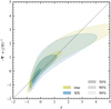 |
Fig. 6 Distributions of velocity divergence versus density contrast values for the true (green) and NN-reconstructed (blue) fields in the validation mocks. They are represented as shaded areas bounded by the iso-density contours of the distribution. Going from a darker to lighter hue, the shaded areas contain 50, 90, and 99% of all the points, respectively. The velocity divergence values are rescaled such that the diagonal dotted line marks the linear theory prediction. |
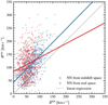 |
Fig. 7 Scatter of true versus NN-reconstructed bulk flow amplitudes of the total survey volume using reconstructions from observations in redshift space (blue) and real space (red) in the validation mocks. The solid lines show the linear regression of true on reconstructed values, with slopes of 1.01 and 0.53 for redshift-space and real-space observations, respectively. For reference, the diagonal is marked with a dotted line. |
4.6 Probing “super-survey” scales
The density field derived from redshift surveys encodes information about “super-survey” mass fluctuations external to the observational volume (Feix & Nusser 2013; Li et al. 2018; Akitsu & Takada 2018; Castorina & Moradinezhad Dizgah 2020). This is because a galaxy’s redshift incorporates its peculiar velocity, which is influenced by the cumulative gravity of the underlying density field both inside and outside the survey volume.
In particular, the bulk flow (mean velocity) of the whole survey volume is influenced by two factors: the gravitational pull of the external mass distribution and a contribution that is proportional to the radius vector of the center of mass inside the survey (Juszkiewicz et al. 1990). The latter term can essentially be interpreted as the net gravitational force exerted on the mass fluctuations inside the survey by the homogeneous background density. Since the density in redshift space is affected by the bulk flow of the entire survey, the NN trained using the full velocity field as target should, at least partially, yield a velocity field that incorporates some constraints on the bulk flow.
Figure 7 presents a scatter plot of the true bulk flow amplitudes Btrue versus NN-reconstructed bulk flow amplitudes ![$\[\hat{B}^{\mathrm{NN}}\]$](/articles/aa/full_html/2024/09/aa50219-24/aa50219-24-eq42.png) , computed from the 640 mock galaxy catalogs of the validation set. The blue points are obtained from our usual NN-reconstructed velocity fields, where the NN was trained on the mock redshift-space observations described in Sect. 2.2. The red points are derived from velocity fields reconstructed by an NN that was trained on mock observations where the distribution of galaxies is given in real space (and no ZoA is imposed).
, computed from the 640 mock galaxy catalogs of the validation set. The blue points are obtained from our usual NN-reconstructed velocity fields, where the NN was trained on the mock redshift-space observations described in Sect. 2.2. The red points are derived from velocity fields reconstructed by an NN that was trained on mock observations where the distribution of galaxies is given in real space (and no ZoA is imposed).
A visual inspection of the blue and red points clearly indicates that Btrue is better correlated with ![$\[\hat{B}^{\mathrm{NN}}\]$](/articles/aa/full_html/2024/09/aa50219-24/aa50219-24-eq43.png) obtained from the distribution of galaxies in redshift space rather than real space. This is confirmed by the Pearson correlation coefficient of 0.59 for the blue points, indicating a strong correlation between Btrue and
obtained from the distribution of galaxies in redshift space rather than real space. This is confirmed by the Pearson correlation coefficient of 0.59 for the blue points, indicating a strong correlation between Btrue and ![$\[\hat{B}^{\mathrm{NN}}\]$](/articles/aa/full_html/2024/09/aa50219-24/aa50219-24-eq44.png) in redshift space. Conversely, the Pearson coefficient for the red points is 0.24, indicative of a weak correlation.
in redshift space. Conversely, the Pearson coefficient for the red points is 0.24, indicative of a weak correlation.
The blue and red straight lines in the figure correspond to linear regressions of Btrue on ![$\[\hat{B}^{\mathrm{NN}}\]$](/articles/aa/full_html/2024/09/aa50219-24/aa50219-24-eq45.png) . The slope of the blue line, obtained from the blue points, is 1.01, indicating a close match between true and reconstructed values in redshift space. Furthermore, the slope of the red line is 0.53, suggesting a less accurate reconstruction for galaxies in real space.
. The slope of the blue line, obtained from the blue points, is 1.01, indicating a close match between true and reconstructed values in redshift space. Furthermore, the slope of the red line is 0.53, suggesting a less accurate reconstruction for galaxies in real space.
The results strongly indicate that the velocity field computed from NN reconstructions in redshift surveys indeed contains constraints on the bulk flow and hence external super-survey fluctuations. The weak correlation seen for reconstruction in real space is mainly the result of the term proportional to the radius vector of the center of mass inside the survey. Additionally, coherence of the density field may also contribute to the correlation seen for reconstructions in real space. Nonetheless, these effects are small compared to the correlation found for the redshift-space reconstruction.
5 Reconstruction from the 2MRS data
After having extensively validated the quality of the NN reconstruction using the mock data in Sec. 4, we are now applying the NN to the 2MRS dataset described in Sec. 2.1. In the following, we analyze the resulting density and peculiar velocity fields, reconstructed within a distance of 200 h−1 Mpc3. As for the mocks, the reconstructed 2MRS fields were all additionally smoothed with a Gaussian window of width rsmooth = 3 h−1 Mpc.
5.1 Cosmography
In Fig. 8, we present the reconstructed 2MRS density and velocity maps, both in the SGP (left panels) and the GP (right panels). For reference, the upper panels show the projected observed galaxy positions in redshift space in a slice extending 5 h−1 Mpc above and below the plane. In the SGP, containing a majority of the dominant structures in the local Universe, a rich distribution of galaxies can be seen near the origin that then rapidly thins out with increasing distance as the fraction of observable galaxies decreases. In the GP, which slices right through the ZoA, only a sparse sample of galaxies is observed near the origin where the ZoA is thinnest.
Maps of the NN-reconstructed density field are plotted in the middle panels of Fig. 8. In the SGP, these maps reveal a vivid contrast of high-density regions, where known clusters reside, as well as filaments and voids. We label some of the dominant clusters that have been successfully reconstructed, listing their names in the figure caption. In the Gp, the reconstructed density map is expectedly less rich in structures. As we have seen for the mock GP in Fig. 2, only the most dominant large-scale structures are expected to be reconstructed, especially in the outer regions where the ZoA becomes wider. Nonetheless, a few known clusters can be identified, two of which, Norma and Perseus-Pisces, are also visible in the SGP. Two additional clusters, Ophiuchus and Triangulum Australis, can be identified with weaker but still pronounced overdensities, the latter at an remarkable distance of about 150 h−1 Mpc deep into the ZoA.
The reconstructed peculiar velocity field, projected onto the plane, is overlaid as arrows. The flow pattern showcases how matter is displaced from under-dense regions into the filamentary structures and then funneled into the dense superclusters. This is particularly prominent in the filament to the top-right of Shapley in the SGP and in the filament to the top-left of Perseus-Pisces in the GP. In general, voids are clearly associated with diverging flows, while the highest overdensities act as main attractors with strongly converging peculiar velocities.
The dominant attractors are most easily identified in the bottom panels of Fig. 8, where we display the reconstructed velocity potential, again overlaid with the velocity field. For this plot, the potential has been offset by a constant such that its average over the whole reconstruction volume vanishes. This way, the sources and sinks of the potential flow clearly correspond to negative and positive potential values, respectively. In the SGP, by far the most dominant attractor is Shapley, displaying a pronounced infall of matter from all directions. But also Coma, Perseus-Pisces and Norma (which is near the center of the Great Attractor) show a notable velocity convergence. Perseus-Pisces and Norma are also highlighted by their convergent flows in the GP. In addition, Triangulum Australis stands out as a dominant attractor in the GP at larger distances from the origin.
For all clusters labeled in Fig. 8 (or their major sub-clusters), we list the coordinates of their NN-reconstructed density peak as well as the NN-reconstructed peculiar velocity at those coordinates in Table 1.
5.2 Bulk flow and Local Group velocity
Given the significant correlation seen between NN-reconstructed and true bulk flows in the validation mocks in Sec. 4.6, we are now investigating the bulk flow derived from the reconstructed 2MRS velocity field. Figure 9 plots the reconstructed bulk flow ![$\[\hat{\boldsymbol{B}}^{\mathrm{NN}}\]$](/articles/aa/full_html/2024/09/aa50219-24/aa50219-24-eq46.png) (solid lines) computed as the volume average of the velocity field
(solid lines) computed as the volume average of the velocity field ![$\[\hat{\boldsymbol{v}}^{\mathrm{NN}}\]$](/articles/aa/full_html/2024/09/aa50219-24/aa50219-24-eq47.png) in spheres of varying radius, showing its amplitude
in spheres of varying radius, showing its amplitude ![$\[\hat{B}^{\mathrm{NN}}\]$](/articles/aa/full_html/2024/09/aa50219-24/aa50219-24-eq48.png) and its three individual components
and its three individual components ![$\[\hat{B}_x^{\mathrm{NN}}, \hat{B}_y^{\mathrm{NN}}\]$](/articles/aa/full_html/2024/09/aa50219-24/aa50219-24-eq49.png) and
and ![$\[\hat{B}_z^{\mathrm{NN}}\]$](/articles/aa/full_html/2024/09/aa50219-24/aa50219-24-eq50.png) , in Galactic coordinates.
, in Galactic coordinates.
The reconstruction errors (shaded areas) were estimated as the standard deviation of the validation mock Btrue values conditioned on a small bin of mock ![$\[\hat{\boldsymbol{B}}^{\mathrm{NN}}\]$](/articles/aa/full_html/2024/09/aa50219-24/aa50219-24-eq51.png) values around those reconstructed from 2MRS. For a selection of radii, the reconstructed bulk flows and their errors are listed in Table 2.
values around those reconstructed from 2MRS. For a selection of radii, the reconstructed bulk flows and their errors are listed in Table 2.
We verify that the 2MRS-reconstructed bulk flow matches the conditional mean true bulk flow ![$\[\left\langle\boldsymbol{B}^{\text {true }} \mid \hat{\boldsymbol{B}}^{\mathrm{NN}}\right\rangle\]$](/articles/aa/full_html/2024/09/aa50219-24/aa50219-24-eq52.png) (dashed lines) in good approximation, as expected for a mean posterior estimate. The minor deviations are a consequence of the finite sample size.
(dashed lines) in good approximation, as expected for a mean posterior estimate. The minor deviations are a consequence of the finite sample size.
The bulk flow amplitude ![$\[\hat{B}^{\mathrm{NN}}\]$](/articles/aa/full_html/2024/09/aa50219-24/aa50219-24-eq53.png) in Fig. 9 first quickly drops from ~590 km s−1 at radius r = 0 to ~220 km s−1 at r = 50 h−1 Mpc, then decreases slowly down to ~90 km s−1 at r = 200 h−1 Mpc. A similar behavior is seen in the individual Cartesian components, of which the Galactic y-component
in Fig. 9 first quickly drops from ~590 km s−1 at radius r = 0 to ~220 km s−1 at r = 50 h−1 Mpc, then decreases slowly down to ~90 km s−1 at r = 200 h−1 Mpc. A similar behavior is seen in the individual Cartesian components, of which the Galactic y-component ![$\[\hat{B}_y^{\mathrm{NN}}\]$](/articles/aa/full_html/2024/09/aa50219-24/aa50219-24-eq54.png) has the dominant contribution.
has the dominant contribution.
Figure 9 also shows, as a red dash-dotted line, the typical bulk flow amplitude expected in a ΛCDM cosmology with the cosmological parameters used in the Quijote simulations and assumed throughout this paper (cf. Sec. 2.2). This expectation was computed as the linear-theory RMS velocity σv(r) in a sphere of radius r via
![$\[\sigma_v^2(r)=\frac{H^2 \Omega_{\mathrm{m}}^{1.1}}{2 \pi^2} \int_0^{\infty} \mathrm{d} k ~P_\delta(k) ~W_{\mathrm{th}}^2(k, r) ~W_{\mathrm{g}}^2(k).\]$](/articles/aa/full_html/2024/09/aa50219-24/aa50219-24-eq55.png) (10)
(10)
Here, Pδ(k) is the matter density contrast power spectrum provided by the Cosmic Emu emulator (Moran et al. 2023), Wth(k, r) is a top-hat window function of radius r, and Wg(k) is a Gaussian window function of width 3 h−1 Mpc, accounting for the field smoothing. Given the uncertainty, the reconstructed bulk flow amplitude is found to be consistent with the ΛCDM expectation within 1 σ for r ≳ 25 h−1 Mpc and within 2 σ for smaller radii.
The bulk flow at r = 0 (first line in Table 2) is simply the reconstructed peculiar velocity with respect to the CMB at the position of the observer, smoothed with a 3 h−1 Mpc wide Gaussian window. It thus provides an estimate of the peculiar velocity of the Local Group. In both amplitude and latitude it is in close agreement with the observed Local Group velocity of vLG = 620 ± 15 km s−1 toward a Galactic longitude and latitude of lLG = 271.9 ± 2.0° and bLG = 29.6 ± 1.4° (Planck Collaboration I 2020a). In longitude it is off by ~18°, which is a 1.8 σ deviation.
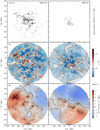 |
Fig. 8 Observed 2MRS galaxies and reconstructed fields in a slice through the Supergalactic (left) and Galactic (right) planes. Top row. redshift-space positions of the observed 2MRS galaxies within a distance of 5 h−1 Mpc to the respective planes. The red cross marks the position of the observer (Local Group) at the origin. Middle row: neural network-reconstructed density (heat map and contours) and peculiar velocity (arrows) fields. The values represented by the contours are marked in the color bar. A reference arrow representing a velocity of 500 km s−1 is shown on the right. Some dominant structures associated with known clusters are labeled by bold black letters: Shapley, Coma, Hydra-Centaurus, Virgo, Norma, Perseus-Pisces, Ophiuchus, Triangulum Australis. Bottom row: NN-reconstructed velocity potential field (heat map and contours) overlaid with the same peculiar velocity field shown in the middle row. |
Positions and peculiar velocities of the NN-reconstructed density peaks that can be identified with known clusters.
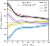 |
Fig. 9 Neural network-reconstructed 2MRS bulk flow amplitude and components (black and colored solid lines, respectively) relative to the CMB in spheres of different radii around the Local Group. The shaded areas mark the 1 σ uncertainty. The conditional mean of the true mock bulk flows given the reconstructed bulk flow is shown as dashed lines. The ΛCDM expectation of the true bulk flow RMS is shown as the red dash-dotted line. For reference, the horizontal dotted line marks a value of zero. |
6 Summary and discussions
In Paper I, preliminary tests were conducted to explore the reconstruction of large-scale structure density and velocity fields using an NN framework. These initial tests involved training and validation data that were derived using approximate gravitational dynamics, which evolved from ΛCDM initial conditions using second-order Lagrangian perturbation theory. Only a simplified RSD model was employed, and galaxy biasing and selection effects were not taken into account. The primary objectives of Paper I were to assess the feasibility of using NNs for modelling the mapping between observations and underlying matter fields, albeit in an approximate form, and crucially, to elucidate the relationship between the reconstructed fields and well-known statistical estimates, namely the mean posterior estimate and the WF.
The current study significantly builds upon Paper I, aiming to develop an NN framework that can be applied to actual observations of the distribution of galaxies in redshift space. This effort involves generating mock catalogs that closely mirror the characteristics of realistic redshift surveys. Specifically, we meticulously created mock catalogs that capture the key features of 2MRS. These catalogs, which are essential for NN training and validation, were derived from the full high-resolution N-body Quijote simulations (Villaescusa-Navarro et al. 2020). They include full RSDs, a nonlinear galaxy bias model, a radially declining selection function, and masking by the ZoA, all calibrated to mimic the properties of the actual 2MRS as closely as possible.
6.1 Method
Our NN is an autoencoder with U-Net architecture, designed to discern the nonlinear mappings between the input observed galaxy number count field and the target true matter density and velocity fields. To achieve this, two separate NNs were trained, each minimizing a customized loss functions designed for predicting either the density or velocity fields. Both loss functions compute a weighted mean squared error between the true and reconstructed fields. Incorporating a distance-dependent weighting into our loss function maintains the property that during training the NN reconstructions converge toward the mean posterior estimate of the true fields given an observation. Our methodology hence results in a robust nonlinear statistical estimator that is computationally expensive to implement with non-machine learning techniques.
We found that customizing the weighting significantly enhanced the NN performance. It accelerated the training convergence and reduced the achieved reconstruction error. The empirically determined weighting is proportional to the selection function, thus accounting for the radially increasing shot noise, and additionally scales with the inverse distance for the velocity reconstruction. Moreover, by assuming potential flow in the loss function for predicting peculiar velocities, we are eliminating the possibility of predicting any unphysical rotational component in the reconstructed velocity field.
Neural network-reconstructed bulk flows in spheres of different radii around the Local Group.
6.2 Validation
Prior to applying our trained models to the 2MRS data, we conducted a comparison with standard WF reconstructions on a validation set of our Quijote-based mocks. This comparison serves as a benchmark for our model, allowing us to discern the advantages and potential limitations of applying an NN instead of a traditional WF.
It was shown in Paper I that the NN consistently outperforms WF in terms of reconstruction accuracy. Similarly, in this study, we find that throughout the survey volume the fields reconstructed by the NN exhibit a lower RMSE compared to those reconstructed by the WF, while also matching the true density and velocity RMS values more closely (cf. Fig. 3). Specifically, the RMSE of the NN-reconstructed density increases from ~0.5 near the observer to ~0.85 at a distance of 200 h−1 Mpc (compared to a true RMS value of ~1.05). Over the same distance range the RMSE of the NN-reconstructed velocity components increases from ~80 to ~200 km s−1 (compared to a true RMS value of ~270 km s−1).
By means of a detailed point-by-point comparison we also demonstrated that the distribution of true versus reconstructed field values is consistently tighter for the NN than for the WF (cf. Figs. 4 and 5). Furthermore, we verified in this comparison that the conditional mean of true field values for a given reconstructed value closely matches that reconstructed value. In other words, the line of linear regression of true on reconstructed field values closely follows the identity line. This demonstrates that the NN reconstruction shows the behavior expected for a mean posterior estimate.
We demonstrated by visual inspection that the NN-reconstructed fields successfully recover the true large-scale structures in the validation mocks, capturing high-density regions, filamentary features and voids, as well as their corresponding converging and diverging velocity flows (cf. Fig. 2).
To explicitly test the capability of the NN in capturing nonlinear effects, we analyzed the distribution of velocity divergence versus density contrast (cf. Fig. 6). We found a good agreement between the true and reconstructed distributions, with both displaying a clear deviation from the linear theory relation.
6.3 Super-survey scales
A galaxy’s peculiar velocity is influenced by the gravitational pull of mass fluctuations outside the survey volume. While the distribution of galaxies in real space remains unaffected by external super-survey scales, the redshift-space density field encodes signatures of these scales through the dependence of galaxy redshifts on peculiar motions.
We showed that our approach to training the NN produces velocity fields that indeed contain information about super-survey scales. This was demonstrated using the validation mock data, through the significant correlation between the bulk flow computed from the reconstructed velocity and the true bulk flow (cf. Fig. 7). This correlation was found only for reconstructions from the distribution of galaxies in redshift space, whereas for reconstructions from real space the correlation was weak. In future work, we intend to train a dedicated NN to predict bulk flows in order to probe super-survey scales more effectively.
6.4 2MRS application
The extensively trained and validated NN was applied to 2MRS, to reconstruct the 3D density and peculiar velocity fields in the local Universe out to a distance of 200 h−1 Mpc. The resulting fields, defined on a regular cubic 128 × 128 × 128 grid of side length 400 h−1 Mpc, as well as their per-grid-point uncertainties, estimated as the RMSE in the mock validation set, are publicly available (cf. footnote 3).
The reconstructed fields recover multiple known clusters, mostly in the SGP, where Shapley is found to be the dominant attractor (cf. Fig. 8). But we also see a few clusters in the GP, which cuts directly through the ZoA. Most notably, despite residing at the edge of the ZoA, Triangulum Australis at a distance of ~150 h−1 Mpc can be identified by a pronounced convergence in the velocity field as well as a minor overdensity in the reconstruction.
From the reconstructed velocity field, we furthermore computed the bulk flow within spheres of varying radii r around the observer (cf. Fig. 9). It shows a remarkable similarity to the bulk flow reconstructed previously in Lilow & Nusser (2021, hereafter LN21). LN21 combined a WF-reconstructed velocity field from 2MRS with an external bulk flow component calibrated by matching the observed peculiar velocities from the galaxy distance catalog Cosmicflows-3 (Tully et al. 2016). In addition, the comparison with Cosmicflows-3 velocities was used to optimize the value of the normalized growth rate fσ8, which determines the peculiar velocity amplitude.
For r ≲ 100 h−1 Mpc, the two bulk flow reconstructions are found to be in 1 to 2 σ agreement. For r ≳ 100 h−1 Mpc, the NN-reconstructed bulk flow amplitude drops more severely than the reconstruction obtained in LN21. This could be the consequence of an only partially captured 2MRS-external bulk flow contribution by the NN. Alternatively or additionally, it might be due to the approximation of the external velocity field contribution in LN21 as a constant (dipole) bulk flow term, which is a better approximation near the center of the reconstruction volume than toward its boundary.
Furthermore, the NN-reconstructed peculiar velocity of the Local Group, corresponding to the bulk flow at r = 0, was found to be ![$\[\hat{v}_{\mathrm{LG}}^{\mathrm{NN}}=587 \pm 84 \mathrm{~km} \mathrm{~s}^{-1}\]$](/articles/aa/full_html/2024/09/aa50219-24/aa50219-24-eq69.png) toward a Galactic longitude and latitude of
toward a Galactic longitude and latitude of ![$\[\hat{l}_{\mathrm{LG}}^{\mathrm{NN}}=254 \pm 10^{\circ}\]$](/articles/aa/full_html/2024/09/aa50219-24/aa50219-24-eq70.png) and
and ![$\[\hat{b}_{\mathrm{LG}}^{\mathrm{NN}}=26 \pm 9^{\circ}\]$](/articles/aa/full_html/2024/09/aa50219-24/aa50219-24-eq71.png) , respectively. This closely matches the observed Local Group velocity of vLG = 620 ± 15 km s−1 toward lLG = 271.9 ± 2.0° and bLG = 29.6 ± 1.4° (Planck Collaboration I 2020a), apart from an 18° deviation in longitude (1.8 σ).
, respectively. This closely matches the observed Local Group velocity of vLG = 620 ± 15 km s−1 toward lLG = 271.9 ± 2.0° and bLG = 29.6 ± 1.4° (Planck Collaboration I 2020a), apart from an 18° deviation in longitude (1.8 σ).
These results are remarkable since our NN reconstruction only uses the 2MRS galaxy redshifts as input. All information about 2MRS-external bulk flow contributions must thus be inferred from their imprint on the observed RSDs.
We need to point out, however, that the reconstructions are dependent on the prior assumptions entering our training mocks, in particular assuming a fixed fiducial ΛCDM cosmology (cf. Sec. 2.2). This fixes the value of the normalized growth rate to fσ8 = 0.444. Training the NN on mocks assuming other values of fσ8 would likely affect at least the amplitude of the reconstructed velocity field. In subsequent work, this could be studied by employing mocks with varying cosmological parameters, for example the latin-hypercube set of Quijote (Villaescusa-Navarro et al. 2020).
6.5 Conclusion
There are evident advantages to using an NN for reconstructions over standard methods. First, the training process does not rely on any approximations for the gravitational dynamics. By incorporating a sufficient number of training data and model parameters, the NN can effectively learn to perform reconstructions by capturing key features of full N-body dynamics, including modified gravity models. In our application, this is clearly demonstrated in Fig. 6, showing the nonlinear relation between the NN-reconstructed velocity and density. This further implies that the NN is capable of probing intermediate (transitional) scales between linear large scales and highly nonlinear small scales. Second, incorporating galaxy bias, RSDs, and selection characteristics of the survey is relatively straightforward in mock catalogs. Consequently, the NN can learn how to extract information while accounting for the limitations of the actual data. Third, by using the appropriate loss and activation functions, an NN can avoid unphysical predictions, such as negative densities or rotational velocity components. These choices can be adapted to any problem and contribute to the NN’s ability to generate consistent and physically relevant results.
In contrast, standard methods often require explicit assumptions about all of these ingredients, which NNs can easily tackle through well-constructed mocks. Given the complexity of these components, standard methods typically resort to simplistic assumptions, which may introduce statistical biases into the inferred information.
Nonetheless, it is crucial to acknowledge that the NN methodology is not without its challenges. For example, acquiring a sufficiently large set of training data, especially when exploring a broad range of cosmological parameters, remains a difficult task. This is in contrast to standard methods, where explicit dependencies on these parameters are incorporated into the approximations that are used, such as the dependence on the background matter density parameter in the velocity-density relationship.
Similarly, accounting for all potentially relevant observational effects is challenging. In constructing the mock data, for example, we did not make a special effort to mimic the properties of the actual Local Group of galaxies. The flow of galaxies in the vicinity of the Local Group is remarkably quiet up to a distance of 5 h−1 Mpc, exhibiting a coherent velocity vLG ≈ 600 km s−1 with respect to the CMB. This coherent flow introduces a strong artificial dipole density enhancement in the distribution of galaxies in redshift space, with redshifts measured in the CMB frame. It is possible to define redshifts with respect to the Local Group motion, which would yield a redshift-space galaxy distribution free from a local dipole enhancement. However, it turns out that it is not possible to extract from the Quijote simulation suite a sufficiently large number of training mocks matching the observed local environment in terms of flow coherence and moderate density. Therefore, we opted to stick to using CMB redshifts since a well-trained NN should in principle be able to learn how to disentangle the artificial local density dipole.
Overall, NN methods offer a wide range of possibilities and enhancements in the field of LSS reconstructions. For example, NN-reconstructed density and velocity maps of the local Universe can improve the extraction of nonlinear cosmographic features, such as filaments, walls, and clusters. The improved reconstructed velocity fields can also be used to test the validity of different gravity models by performing standard comparisons with the observed velocity inferred from distance measurements (e.g. Davis et al. 2011; Turnbull et al. 2012; Ma et al. 2012; Carrick et al. 2015; Said et al. 2020; Boruah et al. 2020; Stahl et al. 2021; Lilow & Nusser 2021; Hollinger & Hudson 2024). Furthermore, NN-reconstructed nonlinear peculiar velocities can be employed for peculiar velocity corrections in local measurements of the Hubble constant using supernovae or other distance measurements (e.g. Peterson et al. 2022; Riess et al. 2022; Kenworthy et al. 2022; Brout et al. 2022). In the future, we plan to extend the applicability of the presented method by training on mocks with a wider range of cosmologies as well as incorporating the observational characteristics and systematics of other surveys.
Acknowledgements
P.G.V. is supported in part at the Technion by a fellowship from the Lady Davis Foundation. We thank Francisco Villaescusa Navarro and Shy Genel for help with the Quijote simulations. This research is supported by a grant from the Israeli Science Foundation and a grant from the Asher Space Research Institute.
References
- Abadi, M., Barham, P., Chen, J., et al. 2016, arXiv e-prints [arXiv:1605.08695] [Google Scholar]
- Akitsu, K., & Takada, M. 2018, Phys. Rev. D, 97, 063527 [NASA ADS] [CrossRef] [Google Scholar]
- Boruah, S. S., Hudson, M. J., & Lavaux, G. 2020, MNRAS, 498, 2703 [Google Scholar]
- Bouchet, F. R., Juszkiewicz, R., Colombi, S., & Pellat, R. 1992, ApJ, 394, L5 [Google Scholar]
- Bouchet, F. R., Colombi, S., Hivon, E., & Juszkiewicz, R. 1995, A&A, 296, 575 [NASA ADS] [Google Scholar]
- Branchini, E., Davis, M., & Nusser, A. 2012, MNRAS, 424, 472 [NASA ADS] [CrossRef] [Google Scholar]
- Brenier, Y., Frisch, U., Hénon, M., et al. 2003, MNRAS, 346, 501 [NASA ADS] [CrossRef] [Google Scholar]
- Brout, D., Scolnic, D., Popovic, B., et al. 2022, ApJ, 938, 110 [NASA ADS] [CrossRef] [Google Scholar]
- Buchert, T., & Ehlers, J. 1993, MNRAS, 264, 375 [Google Scholar]
- Carrick, J., Turnbull, S. J., Lavaux, G., & Hudson, M. J. 2015, MNRAS, 450, 317 [Google Scholar]
- Castorina, E., & Moradinezhad Dizgah, A. 2020, JCAP, 2020, 007 [CrossRef] [Google Scholar]
- Chen, B.-Q., Qin, F., & Li, G.-X. 2024, MNRAS, 528, 7600 [NASA ADS] [CrossRef] [Google Scholar]
- Chen, X., Zhu, F., Gaines, S., & Padmanabhan, N. 2023, MNRAS, 523, 6272 [NASA ADS] [CrossRef] [Google Scholar]
- Chollet, F., et al. 2015, https://github.com/fchollet/keras [Google Scholar]
- Davis, M., & Huchra, J. 1982, ApJ, 254, 437 [NASA ADS] [CrossRef] [Google Scholar]
- Davis, M., Nusser, A., Masters, K. L., et al. 2011, MNRAS, 413, 2906 [Google Scholar]
- Erdoğdu, P., Lahav, O., Huchra, J. P., et al. 2006, MNRAS, 373, 45 [CrossRef] [Google Scholar]
- Feix, M., & Nusser, A. 2013, JCAP, 2013, 027 [CrossRef] [Google Scholar]
- Fisher, K. B., Lahav, O., Hoffman, Y., Lynden-Bell, D., & Zaroubi, S. 1995, MNRAS, 272, 885 [NASA ADS] [Google Scholar]
- Ganeshaiah Veena, P., Lilow, R., & Nusser, A. 2023, MNRAS, 522, 5291 [NASA ADS] [CrossRef] [Google Scholar]
- Goodfellow, I., Bengio, Y., & Courville, A. 2016, Deep Learning (Cambridge, Massachusetts: MIT Press) [Google Scholar]
- Gramann, M. 1993, ApJ, 405, L47 [NASA ADS] [CrossRef] [Google Scholar]
- Hollinger, A. M., & Hudson, M. J. 2024, MNRAS, 531, 788 [NASA ADS] [CrossRef] [Google Scholar]
- Huchra, J. P., Macri, L. M., Masters, K. L., et al. 2012, ApJS, 199, 26 [Google Scholar]
- Jackson, J. C. 1972, MNRAS, 156, 1P [NASA ADS] [CrossRef] [Google Scholar]
- Jasche, J., & Lavaux, G. 2019, A&A, 625, A64 [NASA ADS] [CrossRef] [EDP Sciences] [Google Scholar]
- Juszkiewicz, R., Vittorio, N., & Wyse, R. F. G. 1990, ApJ, 349, 408 [NASA ADS] [CrossRef] [Google Scholar]
- Kenworthy, W. D., Riess, A. G., Scolnic, D., et al. 2022, ApJ, 935, 83 [NASA ADS] [CrossRef] [Google Scholar]
- Kingma, D. P., & Ba, J. 2017, arXiv e-prints [arXiv:1412.6980] [Google Scholar]
- Kitaura, F.-S., Ata, M., Rodríguez-Torres, S. A., et al. 2021, MNRAS, 502, 3456 [NASA ADS] [CrossRef] [Google Scholar]
- Legin, R., Ho, M., Lemos, P., et al. 2024, MNRAS, 527, L173 [Google Scholar]
- Li, Y., Schmittfull, M., & Seljak, U. 2018, JCAP, 2018, 022 [CrossRef] [Google Scholar]
- Lilow, R., & Nusser, A. 2021, MNRAS, 507, 1557 [NASA ADS] [CrossRef] [Google Scholar]
- Linder, E. V. 2005, Phys. Rev. D, 72, 043529 [Google Scholar]
- Ma, Y.-Z., Branchini, E., & Scott, D. 2012, MNRAS, 425, 2880 [Google Scholar]
- Macri, L. M., Kraan-Korteweg, R. C., Lambert, T., et al. 2019, ApJS, 245, 6 [Google Scholar]
- Moran, K. R., Heitmann, K., Lawrence, E., et al. 2023, MNRAS, 520, 3443 [NASA ADS] [CrossRef] [Google Scholar]
- Moutarde, F., Alimi, J.-M., Bouchet, F. R., Pellat, R., & Ramani, A. 1991, ApJ, 382, 377 [Google Scholar]
- Nikakhtar, F., Padmanabhan, N., Lévy, B., Sheth, R. K., & Mohayaee, R. 2023, Phys. Rev. D, 108, 083534 [NASA ADS] [CrossRef] [Google Scholar]
- Nikakhtar, F., Sheth, R. K., Padmanabhan, N., Lévy, B., & Mohayaee, R. 2024, Phys. Rev. D, 109, 123512 [CrossRef] [Google Scholar]
- Nusser, A., & Branchini, E. 2000, MNRAS, 313, 587 [NASA ADS] [CrossRef] [Google Scholar]
- Nusser, A., Dekel, A., Bertschinger, E., & Blumenthal, G. 1991, ApJ, 379, 6 [NASA ADS] [CrossRef] [Google Scholar]
- Planck Collaboration I. 2020a, A&A, 641, A1 [NASA ADS] [CrossRef] [EDP Sciences] [Google Scholar]
- Planck Collaboration VI. 2020b, A&A, 641, A6 [NASA ADS] [CrossRef] [EDP Sciences] [Google Scholar]
- Peebles, P. J. E. 1980, The Large-Scale Structure of the Universe, Princeton Series in Physics (Princeton, N.J: Princeton University Press) [Google Scholar]
- Peebles, P. J. E. 1989, ApJ, 344, L53 [NASA ADS] [CrossRef] [Google Scholar]
- Peterson, E. R., Kenworthy, W. D., Scolnic, D., et al. 2022, ApJ, 938, 112 [NASA ADS] [CrossRef] [Google Scholar]
- Qin, F., Parkinson, D., Hong, S. E., & Sabiu, C. G. 2023, JCAP, 2023, 062 [CrossRef] [Google Scholar]
- Reddi, S. J., Kale, S., & Kumar, S. 2019, arXiv e-prints [arXiv:1904.09237] [Google Scholar]
- Riess, A. G., Yuan, W., Macri, L. M., et al. 2022, ApJ, 934, L7 [NASA ADS] [CrossRef] [Google Scholar]
- Said, K., Colless, M., Magoulas, C., Lucey, J. R., & Hudson, M. J. 2020, MNRAS, 497, 1275 [NASA ADS] [CrossRef] [Google Scholar]
- Sargent, W. L. W., & Turner, E. L. 1977, ApJ, 212, L3 [NASA ADS] [CrossRef] [Google Scholar]
- Schmoldt, I. M., Saar, V., Saha, P., et al. 1999, AJ, 118, 1146 [NASA ADS] [CrossRef] [Google Scholar]
- Shallue, C. J., & Eisenstein, D. J. 2023, MNRAS, 520, 6256 [NASA ADS] [CrossRef] [Google Scholar]
- Stahl, B. E., de Jaeger, T., Boruah, S. S., et al. 2021, MNRAS, 505, 2349 [NASA ADS] [CrossRef] [Google Scholar]
- Tully, R. B., & Fisher, J. R. 1978, in The Large Scale Structure of the Universe (Berlin: Springer), 79, 31 [NASA ADS] [CrossRef] [Google Scholar]
- Tully, R. B., Courtois, H. M., & Sorce, J. G. 2016, AJ, 152, 50 [Google Scholar]
- Turnbull, S. J., Hudson, M. J., Feldman, H. A., et al. 2012, MNRAS, 420, 447 [Google Scholar]
- Villaescusa-Navarro, F., Hahn, C., Massara, E., et al. 2020, ApJS, 250, 2 [CrossRef] [Google Scholar]
- Webster, M., Lahav, O., & Fisher, K. 1997, MNRAS, 287, 425 [Google Scholar]
- Wiener, N. 1949, Extrapolation, Interpolation, and Smoothing of Stationary Time Series: With Engineering Applications (Cambridge, MA: MIT Press) [CrossRef] [Google Scholar]
- Wu, Z., Zhang, Z., Pan, S., et al. 2021, ApJ, 913, 2 [NASA ADS] [CrossRef] [Google Scholar]
- Wu, Z., Xiao, L., Xiao, X., et al. 2023, MNRAS, 522, 4748 [NASA ADS] [Google Scholar]
- Yahil, A., Strauss, M. A., Davis, M., & Huchra, J. P. 1991, ApJ, 372, 380 [NASA ADS] [CrossRef] [Google Scholar]
- Zaroubi, S., Hoffman, Y., Fisher, K. B., & Lahav, O. 1995, ApJ, 449, 446 [Google Scholar]
- Zel’dovich, Ya. B. 1970, A&A, 5, 84 [Google Scholar]
- Zheligovsky, V., & Frisch, U. 2014, J. Fluid Mech., 749, 404 [Google Scholar]
In principle, an NN predicting the individual velocity components should learn their irrotationality during training, since by construction the mean posterior estimate Eq. (5) of irrotational true fields is itself irrotational. In practice, however, the trained NN is not guaranteed to precisely preserve this symmetry, as the NN only approximates the mean posterior estimate.
The reconstructed 3D fields and their uncertainties, estimated as the RMSE in the validation set of mocks, are publicly available at https://github.com/rlilow/2MRS-NeuralNet
All Tables
Positions and peculiar velocities of the NN-reconstructed density peaks that can be identified with known clusters.
Neural network-reconstructed bulk flows in spheres of different radii around the Local Group.
All Figures
|
Fig. 1 Loss functions as a function of training epochs. Left panel: loss function of the reconstructed density field, given in Eq. (6), in the validation (solid blue) and training (dashed light blue) sets of mocks. Right panel: same for the peculiar velocity potential field, given in Eq. (7). |
| In the text | |
|
Fig. 2 Observed, true and reconstructed fields in a slice through the Supergalactic (left) and Galactic (right) planes for one of the validation mocks. Top row: observed galaxy numbers. The red cross marks the position of the observer at the origin. Middle row: true density (heat map and contours) and peculiar velocity (arrows) fields. The values represented by the contours are marked in the color bar. A reference arrow representing a velocity of 500 km s−1 is shown on the right. Bottom row: corresponding NN-reconstructed fields. |
| In the text | |
|
Fig. 3 Root mean square (top) and root mean squared error (bottom) of the reconstructed fields as a function of distance. Top-left panel: root mean square of the reconstructed density contrast for the NN (blue) and WF (orange) in the validation mocks. The RMS is averaged over spherical shells of width 10 h−1 Mpc. For reference, the RMS of the true field is marked by the horizontal dotted line. Top-right panel: same for the radial (solid) and tangential (dashed) peculiar velocity components. Bottom row: same for the root mean squared error. |
| In the text | |
|
Fig. 4 Distribution of true versus reconstructed field values. Left panel: distribution of true versus reconstructed density values for the NN (blue) and WF (orange) reconstructions in the validation mocks, represented as shaded areas bounded by the iso-density contours of the distribution. Going from a darker to lighter hue, the shaded areas contain 50, 90, and 99% of all the points, respectively. The conditional mean true values and the 68% most likely true values for a given reconstructed value are shown as solid lines and error bars, respectively. The average reconstructed values for a given true value are shown as dashed lines (understood as a function of the true values). For reference, the diagonal is marked with a dotted line. Right panel: same for the peculiar velocity components. |
| In the text | |
|
Fig. 5 Conditional distributions of true given reconstructed field values. Top-left panel: conditional distribution of true densities for a given reconstructed density |
| In the text | |
|
Fig. 6 Distributions of velocity divergence versus density contrast values for the true (green) and NN-reconstructed (blue) fields in the validation mocks. They are represented as shaded areas bounded by the iso-density contours of the distribution. Going from a darker to lighter hue, the shaded areas contain 50, 90, and 99% of all the points, respectively. The velocity divergence values are rescaled such that the diagonal dotted line marks the linear theory prediction. |
| In the text | |
|
Fig. 7 Scatter of true versus NN-reconstructed bulk flow amplitudes of the total survey volume using reconstructions from observations in redshift space (blue) and real space (red) in the validation mocks. The solid lines show the linear regression of true on reconstructed values, with slopes of 1.01 and 0.53 for redshift-space and real-space observations, respectively. For reference, the diagonal is marked with a dotted line. |
| In the text | |
|
Fig. 8 Observed 2MRS galaxies and reconstructed fields in a slice through the Supergalactic (left) and Galactic (right) planes. Top row. redshift-space positions of the observed 2MRS galaxies within a distance of 5 h−1 Mpc to the respective planes. The red cross marks the position of the observer (Local Group) at the origin. Middle row: neural network-reconstructed density (heat map and contours) and peculiar velocity (arrows) fields. The values represented by the contours are marked in the color bar. A reference arrow representing a velocity of 500 km s−1 is shown on the right. Some dominant structures associated with known clusters are labeled by bold black letters: Shapley, Coma, Hydra-Centaurus, Virgo, Norma, Perseus-Pisces, Ophiuchus, Triangulum Australis. Bottom row: NN-reconstructed velocity potential field (heat map and contours) overlaid with the same peculiar velocity field shown in the middle row. |
| In the text | |
|
Fig. 9 Neural network-reconstructed 2MRS bulk flow amplitude and components (black and colored solid lines, respectively) relative to the CMB in spheres of different radii around the Local Group. The shaded areas mark the 1 σ uncertainty. The conditional mean of the true mock bulk flows given the reconstructed bulk flow is shown as dashed lines. The ΛCDM expectation of the true bulk flow RMS is shown as the red dash-dotted line. For reference, the horizontal dotted line marks a value of zero. |
| In the text | |
Current usage metrics show cumulative count of Article Views (full-text article views including HTML views, PDF and ePub downloads, according to the available data) and Abstracts Views on Vision4Press platform.
Data correspond to usage on the plateform after 2015. The current usage metrics is available 48-96 hours after online publication and is updated daily on week days.
Initial download of the metrics may take a while.