| Issue |
A&A
Volume 689, September 2024
|
|
|---|---|---|
| Article Number | A353 | |
| Number of page(s) | 11 | |
| Section | Cosmology (including clusters of galaxies) | |
| DOI | https://doi.org/10.1051/0004-6361/202450007 | |
| Published online | 24 September 2024 | |
Planck data revisited: Low-noise synchrotron polarization maps from the WMAP and Planck space missions
1
CNRS-UCB International Research Laboratory, Centre Pierre Binétruy,
IRL 2007, CPB-IN2P3,
Berkeley,
CA
94720,
USA
2
Lawrence Berkeley National Laboratory,
1 Cyclotron Road,
Berkeley,
CA
94720,
USA
Received:
17
March
2024
Accepted:
24
April
2024
Abstract
Context. Observations of cosmic microwave background (CMB) polarization, essential for probing a potential phase of inflation in the early Universe, suffer from contamination by polarized emission from the Galactic interstellar medium.
Aims. This work combines existing observations from the WMAP and Planck space missions to make a low-noise map of polarized synchrotron emission that can be used to clean forthcoming CMB observations.
Methods. We combine DR5 K, Ka and Q WMAP maps with PR4 30 and 44 GHz Planck LFI maps, using weights that near-optimally combine the observations as a function of sky direction, angular scale, and polarization orientation.
Results. We publish well-characterized maps of synchrotron Q and U Stokes parameters at ν = 30 GHz and an angular resolution of 1 degree. A statistical description of uncertainties is provided with Monte-Carlo simulations of additive and multiplicative errors.
Conclusions. Our maps are the most sensitive full-sky maps of synchrotron polarization to date, and are made available to the scientific community on a dedicated website.
Key words: ISM: general / ISM: magnetic fields / Galaxy: general / cosmic background radiation / cosmology: observations / inflation
Corresponding author; This email address is being protected from spambots. You need JavaScript enabled to view it.
© The Authors 2024
 Open Access article, published by EDP Sciences, under the terms of the Creative Commons Attribution License (https://creativecommons.org/licenses/by/4.0), which permits unrestricted use, distribution, and reproduction in any medium, provided the original work is properly cited.
This article is published in open access under the Subscribe to Open model. This email address is being protected from spambots. You need JavaScript enabled to view it. to support open access publication.
1 Introduction
The cosmic microwave background (CMB), relic radiation emitted when electrons and nuclei first combined to form neutral atoms, has been transformational for understanding the origin, evolution, and matter and energy content of the Universe we live in. Observations from a series of space-borne (Smoot et al. 1992; Mather et al. 1994; Bennett et al. 2013; Planck Collaboration I 2020), balloon-borne (e.g., Hanany et al. 2000; Netterfield et al. 2002; Benoît et al. 2003), and ground-based (e.g., Das et al. 2014; BICEP2 Collaboration 2016; Louis et al. 2017; POLARBEAR Collaboration 2017; Henning et al. 2018) CMB experiments, complemented by other cosmological probes (e.g., Perlmutter et al. 1999; Eisenstein et al. 2005; Alam et al. 2017; Abbott et al. 2022), have led to a standard cosmological scenario, inflationary ΛCDM, in which an expanding universe is filled today with about 30% pressureless matter and 70% dark energy. In this paradigm, galaxies and clusters of galaxies form from initial density perturbations generated during an early phase of rapid expansion, dubbed cosmic inflation. The fast expansion in the inflationary phase expands tiny local quantum fluctuations of the spacetime metric to supra-horizon scales, and these later on reenter the horizon and seed the gravitational collapse of structures observable today (Bardeen et al. 1983). While appealing, the inflationary hypothesis still requires observational confirmation, as well as the identification of the correct model from a plethora of viable alternatives (Martin et al. 2014).
In many inflationary models, initial perturbations of the spacetime metric comprise, in addition to a scalar term corresponding to initial density perturbations responsible for the formation of the large-scale structures, a tensor term corresponding to primordial gravitational waves. These tensor modes of metric perturbation are expected to imprint, on the CMB, tiny fluctuations of polarization of the B-mode type (of odd parity), while density perturbations generate, at the time of CMB emission, only E-mode type polarization (of even parity). For this reason, the detection of primordial B modes of CMB polarization is considered an essential next step in observational cosmology (Kamionkowski & Kovetz 2016). If detected with an angular power spectrum matching theoretical prediction, they would be a “smoking gun” for cosmic inflation. This motivates the deployment of ambitious next-generation CMB observatories, on the ground and in space, dedicated to the detection of primordial CMB polarization B-modes (Hui et al. 2018; Ade et al. 2019; Abazajian et al. 2019; Delabrouille et al. 2018; Hanany et al. 2019; LiteBIRD Collaboration 2023).
The amplitude of primordial gravitational waves, parameterized by the tensor-to-scalar ratio, r, is already constrained by existing CMB observations to r ≤ 0.036 and r ≤ 0.032 at 95% CL, in two recent independent analyses combining Planck and BICEP/Keck data (BICEP/Keck 2022; Tristram et al. 2022). At this level and below, over most of the sky, for most of the harmonic scales, and at all observing frequencies, CMB B-mode fluctuations are fainter than fluctuations of microwave polarized emission originating from the interstellar medium (ISM) of our own Milky Way. Two processes of ISM emission are known to contribute a significant amount of microwave polarization. Elongated galactic dust grains, aligned preferentially perpendicularly to the local Galactic magnetic field, polarize the light from background stars parallel to the local Galactic magnetic field (Davis & Greenstein 1951), and emit polarized microwave emission perpendicular to the magnetic field. Polarized dust emission in the microwave and submillimeter has been detected at 353 GHz by the Archeops stratospheric balloon (Benoît et al. 2004), and in several frequency bands by the high-frequency instrument (HFI) aboard the Planck space mission (Planck Collaboration XI 2020; Planck Collaboration IV 2020). At lower frequencies, energetic electrons in the ionized ISM spiralling in the Galactic magnetic field generate synchrotron emission that is highly polarized. This polarized synchrotron emission has been mapped over the full sky, although with a limited signal-to-noise ratio at high galactic latitudes, by the WMAP space mission (Kogut et al. 2007), and by the low-frequency instrument (LFI) aboard the Planck satellite (Planck Collaboration IX 2016; Planck Collaboration IV 2020).
Future suborbital CMB observations, such as those planned with the BICEP array (Hui et al. 2018), the Simons observatory (Ade et al. 2019), AliCPT (Salatino et al. 2020), or with the future CMB-S4 experiment (Abazajian et al. 2019), must monitor the contamination of CMB observations by Galactic dust and Galactic synchrotron polarization. To that effect, one may envisage using existing data from WMAP and Planck to help model and subtract polarized emission from the ISM in ground-based CMB observations. Template maps for polarized dust and synchrotron emission have been produced with a component separation pipeline from the final Planck space mission data (Planck Collaboration IV 2020), and made available to the scientific community in the Planck space mission legacy archive at ESA1. These maps, however, suffer from limitations, some of which can be addressed by making better use of existing data.
The main limitation of the published WMAP and Planck polarized synchrotron maps is the level of instrumental noise. In particular, maps are strongly noise-dominated in regions of sky with the lowest Galactic foreground emission, which would be the main targets for upcoming ground-based observations. This comes from the limited sensitivity of existing surveys, and from the fact that published maps do not best combine all existing observations; the latest Planck published synchrotron maps (Planck Collaboration IV 2020), for instance, use only Planck data.
In this paper, we combine WMAP and Planck LFI data in a simple yet near-optimal way, to produce well-characterized maps of the Q and U Stokes parameters of “Planck-revisited” polarized synchrotron emission at 30 GHz, which can be used for foreground cleaning in upcoming CMB observations with ground-based experiments. While our paper was in preparation, Watts et al. (2024) have combined Planck and WMAP observations to produce 30 GHz maps of polarized synchrotron emission amplitude with noise levels lower than those of the WMAP K channel alone, using a conceptually different approach. Data products are part of the Cosmoglobe first data release (Cosmoglobe DR1). In that analysis, Watts et al. (2024) use a pipeline that first corrects for a model of systematic residuals in WMAP data and for calibration uncertainties in Planck HFI data, and then fits for a multicomponent model of sky emission in multifrequency maps. However, our focused pipeline has specific advantages, which we discuss in this paper. In particular, our data products have a better signal-to-noise ratio in regions of low foreground contamination, and their effective angular resolution is better characterized. The increased sensitivity is of specific interest for ground-based experiments targeting primordial B-mode detection in patches of sky with low foreground emission, such as the Simons Observatory (Ade et al. 2019), various generations of BICEP/Keck (Hui et al. 2018; Schillaci et al. 2020), and AliCPT (Salatino et al. 2020).
The rest of the paper is organized as follows. In Sec. 2, we describe the input WMAP and Planck observations that are used in this work. In Sec. 3, we describe the data pipeline that is used to combine those observations to make a single map of polarized synchrotron emission at a frequency of 30 GHz. Section 4 gives and discusses the main results and data products made available to the scientific community. We conclude in Sec. 5.
2 Input observations and modeling assumptions
WMAP, launched in June 2001 by NASA, has observed the full microwave sky in five frequency bands, centered from 23 to 94 GHz. The Planck space mission has observed the sky in nine frequency bands centered at frequencies ranging from 27 to 857 GHz.
In this paper, we use DR5 (9-year) WMAP data release polarization maps for the K, Ka, and Q bands (Bennett et al. 2013), and Planck DR4 LFI 30 and 44 GHz data (Planck Collaboration Int. LVII 2020). Contamination by polarized dust emission at these frequencies is strongly subdominant as compared to either synchrotron emission or instrumental noise. We do not use the WMAP V and W bands, which have a low synchrotron signal-to-noise ratio over the largest fraction of sky, or the 70 GHz Planck LFI map or any of the Planck HFI maps, which provide little additional information for mapping polarized synchrotron specifically, and may contain non-negligible polarized dust emission. However, we do make use of the CMB temperature and polarization maps obtained with the spectral matching independent component analysis (SMICA) method (Delabrouille et al. 2003; Cardoso et al. 2008) to correct the low-frequency maps from a subdominant CMB polarization contamination.
To first order, synchrotron emission, s(ν), scales in frequency proportionally to a power of frequency; that is, for each sky pixel,
![Mathematical equation: $\[s(\nu) \propto \nu^{\beta_s} .\]$](/articles/aa/full_html/2024/09/aa50007-24/aa50007-24-eq1.png) (1)
(1)
The spectral index, βs, depends on the spectral energy distribution of the relativistic electrons, and is hence theoretically supposed to depend on the physical properties of the region of emission.
In the frequency range of interest, a simple power law with fixed βs ≃ −3.1 (when the emission is expressed in antenna temperature (KRJ) units) is a good approximation, but there is evidence of slight variations, δβs ≃ ±0.1, as a function of the direction in the sky (Krachmalnicoff et al. 2018; de la Hoz et al. 2023; Watts et al. 2024). More generally, the power-law scaling approximation can break down at higher frequencies; for example, because of a depletion of high-energy electrons, leading to a possible steepening of the frequency dependence. At low frequencies, below ν ~ 5 GHz, Faraday rotation of polarization, and line-of-sight integration leads to depolarization that renders this power law invalid for the Q and U Stokes parameters. Several authors have attempted to map the synchrotron spectral index using existing datasets, but the results are noisy and uncertain (see, e.g., Krachmalnicoff et al. 2018; Fuskeland et al. 2021; de Belsunce et al. 2022; Weiland et al. 2022; de la Hoz et al. 2023; Watts et al. 2024, for recent results). Spectral index maps obtained using intensity observations in the frequency domain of interest suffer from contamination by dust “anomalous microwave emission” (AME) and free-free emission, which are hard to separate from synchrotron by reason of a lack of observing frequencies. Spectral index maps obtained from polarization data, negligibly impacted by AME and free-free that are at most very faintly polarized, are either contaminated by large-scale systematic effects due to intensity to polarization leakage, or suffer from Faraday rotation effects and/or a poor signal-to-noise ratio.
For the work presented here, we assume a fixed synchrotron spectral index of βs = −3.1. Table 1 gives the frequency scaling of synchrotron for several values of the spectral index, normalized to unity at 30 GHz. Relative differences from 23 to 44 GHz are in the range of a few percent. Errors made by using a fixed spectral index are thus on the order of a few percent of the total emission. Further discussion of the impact of this choice is deferred to Sec. 4.1.
Synchrotron emission scaling with frequency.
3 Method
The present works aims to combine WMAP and Planck synchrotron observations for an increased signal-to-noise ratio. For both WMAP and Planck, the noise level strongly depends on the sky pixel considered (Figs. 1 and 2).
By reason of frequency-dependent angular resolution, it also depends on angular scale (Fig. 3). Finally, it depends on the Stokes parameter being considered, Q or U. We hence propose to combine the observations using relative weights that depend on sky direction, harmonic mode, and polarization orientation. This is done using a decomposition of the maps onto a needlet frame. The so-called “needlets” are a kind of wavelet defined on the sphere. For our purpose, needlet decomposition was performed by filtering the original maps in a set of harmonic windows, hJ(ℓ), where J indexes the scale and ℓ is the harmonic mode of spherical harmonics transforms (SHTs). These needlet windows were normalized so that
![Mathematical equation: $\[\sum_J h_J(\ell)^2=1\]$](/articles/aa/full_html/2024/09/aa50007-24/aa50007-24-eq2.png) (2)
(2)
over a useful range of ℓ. Maps of needlet coefficients were obtained by an inverse SHT on the filtered harmonic coefficients. Map reconstruction from the needlets was done by again filtering each needlet coefficient map by the corresponding spectral window, co-addition in harmonic space, and an inverse SHT of the recombined aℓm coefficients.
Stokes parameter, Q and U, maps are defined with respect to a set of axes. They are not invariant with a transformation of those local reference axes. For this reason, they are not scalar quantities, but spin-2 fields. In CMB data analysis, it is customary to decompose polarization maps into an alternate basis, the E and B polarization modes, respectively, scalar (even parity) and pseudo-scalar (odd parity). In previous work using needlets for polarization, needlet windows have been used to filter E and B fields, which are then transformed into needlet coefficient maps for E and B, processed, and then recombined. While this makes sense for the analysis of CMB maps, for which E modes and B modes are a natural decomposition, with E modes outshining B modes by orders of magnitude, it is not the case for maps of Galactic foreground components, for which E and B modes are on the same order of magnitude and have no special theoretical justification. On the contrary, the transformation of Q and U into E and B is nonlocal (while foreground emission is), and does also suboptimally smooth the inhomogeneity of the noise level (the standard deviation is pixel-dependent). Moreover, the noise level is different in Q and U maps, as it depends on the orientation of the detectors as they scan through the sky pixels, a property that should be taken into account for the use of optimal weights in the production of low-noise maps.
In this work, noise-weighted combinations were performed pixel by pixel in needlet coefficient maps, but instead of working on needlet coefficients for E and B, as was done in previous work (Basak & Delabrouille 2013; Aurlien et al. 2023; Errard et al. 2022), we transformed back E and B maps filtered by the spectral windows, hJ(ℓ), into maps of Q and U, made noise-weighted combinations of those “special needlets” in pixel space, transformed them back into E and B aℓms, which were then filtered again by the spectral windows and co-added to produce Q and U synchrotron maps with near-optimal signal-to-noise ratios.
The specific data-processing pipeline set up in this work is summarized as follows:
Planck 30 and 44 GHz frequency maps, and WMAP K, Ka, and Q maps were smoothed to an angular resolution of 60′ in harmonic space;
CMB polarization was subtracted from all frequency maps to minimize residual CMB in the maps;
All maps were rescaled to equivalent synchrotron emission at the 30 GHz reference frequency, assuming a power law frequency scaling with spectral index βs = −3.1;
We computed needlet coefficients by filtering E and B aℓms using a set of 20 bands spanning the ℓ = 2–1000 range of harmonic modes, and producing corresponding maps of Q and U needlets at nside=512;
We computed the noise level of each frequency channel in this needlet space, as a function of scale and sky pixels, and got inverse variance-weighted averages for Q and U in each needlet band;
Those needlet coefficients were then used to reconstruct a single map of synchrotron Q and U polarization at an angular resolution of 60′, which could be used as a template for polarized synchrotron emission at 30 GHz;
Two hundred maps of simulated noise for the end product were obtained by co-adding WMAP and Planck noise simulations to the weights used in the production of the polarized synchrotron maps.
Each of these steps is further detailed in the following subsections.
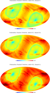 |
Fig. 1 Noise standard deviation maps for the three WMAP channels used in this work (K, Ka and Q), rescaled to equivalent 30 GHz noise assuming a synchrotron spectral index of −3.1. Units are in μKcmb. Each map displays the average of the standard deviation of the Q and U Stokes parameter maps. |
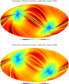 |
Fig. 2 Noise standard deviation maps for the two Planck LFI channels used in this work (30 and 44 GHz), rescaled to equivalent 30 GHz noise assuming a synchrotron spectral index of −3.1. Units are in μKcmb. Each map displays the average of the standard deviation of the Q and U Stokes parameter maps. Here and in Fig. 1, different color scales have been used for the different frequency channels. We note that the noise level for each channel is variable across the sky, and that the shape and location of the lowest-noise regions is channel-dependent. The map depth varies by an order of magnitude across the sky, and the lowest-noise regions are different between the maps. This calls for pixel-dependent weights for map combination. |
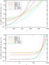 |
Fig. 3 Beam-corrected noise spectra for the WMAP and Planck channels used in this work, rescaled to equivalent 30 GHz noise assuming a synchrotron spectral index of −3.1. The relative sensitivity of the different channels strongly depends on the harmonic scale, ℓ. On the largest scales, the WMAP K band and the LFI 30 GHz channels have a comparable mean synchrotron sensitivity (with, however, a strong pixel dependence, as is seen in Figs. 1 and 2. At ℓ ≃ 800, however, the WMAP Q and LFI 44 GHz are about as sensitive as the LFI 30 GHz channel, and much more sensitive than the WMAP K band. |
3.1 Step 1: Map smoothing
Original WMAP and Planck maps used in this work have angular resolutions ranging from about 27.9′ (for the Planck LFI 44 GHz band, with the best resolution of the five) to about 52.8′ (for the WMAP K band). As a first step, we transformed original maps into spherical harmonics, and filtered the map aℓms by the ratio of the Bℓ of a 60′ beam and the Bℓ of the original map. For WMAP, we used the tabulated beam Bℓs provided with the WMAP DR5. For the Planck LFI, we assume that the original beams are 33.1′ and 27.9′ for the 30 and 44 GHz, respectively. Small differences between those assumed values and the actual beams (which are known to be somewhat elliptical) have little impact on the final products, for which high-ℓ power is further suppressed.
The choice of 60′ as the final resolution is motivated by an inspection of the power spectrum of the initial maps, which is noise-dominated above values of ℓ ranging from ℓ = 200 at best (for near-full sky LFI 30 GHz maps) to ℓ = 20–30 at worst (for high Galactic latitude maps at 44 GHz and in the WMAP Q band). The whole pipeline has also been run with a 50′ and 40′ target resolution, but the maps produced are noisier and contain little extra signal information in regions of faint emission2.
3.2 Step 2: Cosmic microwave background subtraction
All of the maps used in this work contain some CMB polarization. This CMB “contamination” is subdominant compared to synchrotron emission and to noise contamination, but for the sake of optimality we subtracted from each of the maps a Wiener-filtered version of the SMICA polarization maps. Multivariate Wiener filtering was performed, assuming theoretical CMB intensity and polarization spectra corresponding to the best-fit Planck cosmological model. The multivariate spectrum of the noisy CMB maps was computed directly on the SMICA maps. Subtracting a Wiener-filtered CMB (rather than the SMICA CMB polarization maps themselves) ensures that CMB subtraction does not add more noise than it subtracts CMB. The residual noise in the maps is subdominant and, since it originates predominantly from HFI observations, is not significantly correlated with original noise in the WMAP and LFI channels. Its contribution, as well as that of the residual CMB, can safely be neglected in the computation of the weights to be used for the production of the synchrotron map.
We do not describe this step in more detail as it has almost no impact on the final products. Synchrotron Q and U maps have been produced with pipelines including or omitting CMB subtraction. The rms of the difference between the two solutions is 0.47 μKRJ, compared to a noise level of 2.78 μKRJ in the final polarized intensity map with CMB subtracted. Still, one should be aware that there is low-level residual CMB in the final products, even for the pipeline that includes CMB subtraction (the difference between the Wiener-filtered CMB and the original CMB is present in the maps). This residual can be characterized precisely if necessary for specific analyses3.
3.3 Step 3: Rescaling to 30 GHz reference frequency
After the two previous steps, we are left with five noisy synchrotron-dominated sky maps, all of which share the effective angular resolution of a 1-degree Gaussian beam over their common range of used ℓ values. For each of them, the useful ℓ range is restricted by the availability or accuracy of the instrumental effective beam window functions. We used ℓmax = [700, 750, 1000, 850, 1000] for WMAP K, Ka, Q, and LFI 30 and 44 GHz, respectively.
We then used the WMAP and LFI band-passes to integrate a single power law with a spectral index of −3.1 (in KRJ units) and used the corresponding synchrotron band-pass-integrated coefficients to rescale each map to equivalent synchrotron emission at 30 GHz (Table 1). This rescaling, by reason of variation in the synchrotron spectral index (or more generally, the synchrotron frequency scaling) across the sky, is slightly inaccurate. We evaluated the amplitude of the errors by computing the scaling coefficients for spectral indices ranging from −2.9 to −3.3. Differences of a few percent at most across the frequency channels guarantee that scaling errors are at most a few percent of the total signal (and in practice less, taking averaging between input maps on both sides of the reference frequency into account). These errors are below the noise over most of the sky, the only exception being regions of emission with a signal-to-noise ratio of a few tens or more (in amplitude), for which there is no need to use the synchrotron maps produced in this paper rather than the original observations. We evaluate uncertainties more rigorously in Sec. 4.
3.4 Step 4: Needlet coefficients
The CMB-corrected maps, smoothed to a resolution of 60′ and scaled to 30 GHz synchrotron assuming a βs = −3.1 spectral index, were filtered in a set of cosine-shaped “needlet bands” shown in Fig. 4. These were chosen to be wide enough to allow for localization on the scale of about a degree, allowing for weights to be adapted to map depth inhomogeneities on that scale. They are narrow enough for the signal-to-noise ratio of the various channels not to vary too much in each band.
In practice, Q and U maps in each channel were transformed into E and B aℓms, which were then multiplied by the windows, hJ(ℓ), and transformed back using an inverse polarized SHT to produce a number, NJ, of each of the Q and U needlet coefficient maps.
3.5 Step 5: Inverse noise variance weighting
For each “needlet” map of Q and U Stokes parameters, we estimate the local noise variance integrated in the band. This was done by multiplying the original noise level in the map space by a rescaling factor that takes into account noise reduction in the band by reason of map smoothing (i.e., that takes into account the ratio of the beam, Bℓ, squared, integrated in the needlet band). We then co-added the needlet maps for the various channels with weights proportional to 1/σ2, normalized for unit response. This gives us 20 maps of needlet coefficients for each of Q and U, which near-optimally combine the five original WMAP and LFI Q and U needlet coefficients for that scale into one single map of synchrotron emission needlet coefficients for each of Q and U at 30 GHz.
The relative weights for the various channels depend on the needlet scale (WMAP K and LFI 30 GHz dominate the weights on a large scale, while other channels contribute on a smaller scale), on the sky pixel, and on the Stokes parameter (the weights are different for Q and U, because the noise levels in each of those depend on the orientation of the scanning with respect to local polarization reference axes). While it may seem that the WMAP Ka and Q bands, and the LFI 44 GHz channel, have subdominant weights except on the smallest scales, they are actually relevant even on degree scales in localized patches of deep integration, which are slightly shifted between the various frequency channels (by reason of focal plane arrangements and scanning geometry). Keeping them in the analysis increases a bit the extent of patches of deeper integration in the final combined map.
For illustration purposes, weights for the WMAP K band and the LFI 30 GHz channel, for the first needlet scale, are shown in Fig. 5. In regions near the ecliptic poles, most of the weight is given to the LFI 30 GHz map, while over a large fraction of the sky, the WMAP K channel has a larger weight in the reconstruction.
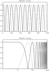 |
Fig. 4 Cosine-shaped needlet bands, hJ(ℓ), used in this work. As usual, those are normalized so that ∑J hJ(ℓ)2 = 1 for a useful range of ℓ. Here, this normalization holds up to ℓ = 950. For higher ℓ, the sum goes smoothly to zero at ℓmax = 1000 with a cosine-square half-arch. |
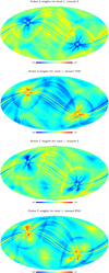 |
Fig. 5 Weights used for the reconstruction of the synchrotron Q (top two) and U (bottom two) synchrotron polarization maps in the first needlet band. Only the weights of the WMAP K and the Planck LFI 30 GHz maps are shown, as only those are significant for that scale (and add up to almost one). We note the differences between Q and U weights. |
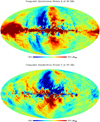 |
Fig. 6 Stokes Q (top) and U (bottom) 30 GHz polarization maps obtained with the pipeline described in this paper, at an angular resolution of 1 degree. |
3.6 Step 6: Co-addition
Maps of needlet coefficients for Q and U were straightforwardly recombined into co-added maps as usual: polarized SHTs were performed to transform needlet Q and U maps into E and B aℓm for each band. Those aℓms were each multiplied by the appropriate needlet window, hJ(ℓ). Those were then co-added before a final inverse SHT was performed to get the final Q and U synchrotron maps with all the scales co-added.
3.7 Step 7: Noise simulations
Synchrotron maps obtained following the previous steps comprise noise from WMAP and Planck observations, combined in a nontrivial way (with a nonstationary, scale-dependent, polarization-orientation-dependent contribution from the various channels). This noise is not easily characterized analytically, as it is also correlated between pixels due to smoothing of the original observations. Two hundred simulated noise maps were obtained by projecting WMAP and Planck LFI simulated noise using the weights used for the various channels as a function of sky pixel and scale. For each simulation, random noise was generated using pixel-based covariance matrices for the I, Q, and U noise provided by the WMAP and Planck collaborations, produced at the native nside and angular resolution. These noise maps were then smoothed to an angular resolution of 60′, rescaled to 30 GHz using the synchrotron frequency scalings, decomposed into Q and U needlets, and weighted and recombined into a single noise realization. The statistics across the 200 realizations are sufficient to characterize noise contamination properties with an error of a few percent, and global statistics (i.e., noise rms, spectrum) with sub-percent accuracy.
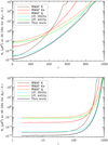 |
Fig. 7 Beam-corrected noise spectra for the WMAP and Planck channels used in this work, rescaled to equivalent 30 GHz noise assuming a synchrotron spectral index of −3.1, as in Fig. 3. An extra black curve shows the noise spectrum of the final composite synchrotron map obtained in this work, which near-optimally combines all observations. |
4 Results, discussion, and data products
The main final data product is a pair of estimated Q and U synchrotron emission maps at 30 GHz, with a 1 degree Gaussian beam angular resolution. Maps of Q and U are shown in Fig. 6. The co-addition of the original WMAP and Planck LFI observations using weights that depend on sky pixels and on angular scale for each of Q and U independently allows for a significantly improved signal-to-noise ratio compared to any of the original input maps.
Figure 7 compares the E and B noise spectra of the final synchrotron polarization obtained in this work to the original noise level of the input WMAP and Planck LFI channels (all rescaled to 30 GHz assuming a synchrotron spectral index of βs = −3.1). As was expected, the noise of our final synchrotron maps is lower than any of the noise spectra of the input maps used in this analysis.
Figure 8 shows a map of synchrotron polarized amplitude, together with a map of noise standard deviation obtained from 200 simulated noise maps. Low-noise regions corresponding to both WMAP and Planck deeper integration zones are clearly visible in the standard deviation map, showing how the present method takes the best of the various observations used.
No specific attempt has been made to subtract point source emission in either the initial maps or the final polarization maps. Well-known bright radio sources can be identified in the final map. This is the case for supernova remnants in our own Galaxy such as Tau A and Cas A, for bright radio galaxies such as Cen A, Fornax A, and Virgo A, and for bright distant quasars such as 3C273 and 3C279. A catalog of polarized radio sources detected with Planck is available for identification and masking. Since the emissions from these sources do not necessarily scale with frequency with a power law with a spectral index of −3.1, their flux in the maps is not expected to correspond to their true 30 GHz emission. For convenience, a compact source mask (shown in Fig. 9) is made available as part of the data products.
We anticipate that the present maps can be used as synchrotron polarization Q and U templates for foreground cleaning in upcoming CMB observations, in particular at angular scales of a few degrees to detect primordial B-modes of CMB polarization. They will also be useful for making new models of Galactic foregrounds to be used in sky simulation tools such as the PSM (Delabrouille et al. 2013) and the PySM (Thorne et al. 2017; Zonca et al. 2021), to be used for the development of data analysis pipelines in preparation for future observations at millimeter to centimeter wavelengths. The good characterization of the maps in terms of the effective beam and the availability of 200 noise simulations will make it easy to combine the map with independent observations for further improvements.
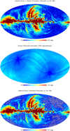 |
Fig. 8 Synchrotron and noise polarized intensity obtained in this work. Top: total polarized intensity, |
![Mathematical equation: $\[P=\sqrt{Q^2+U^2}\]$](/articles/aa/full_html/2024/09/aa50007-24/aa50007-24-eq3.png)
![Mathematical equation: $\[\left(Q^2+U^2\right)-\left(\sigma_Q^2+\sigma_U^2\right)\]$](/articles/aa/full_html/2024/09/aa50007-24/aa50007-24-eq4.png)
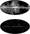 |
Fig. 9 Masks used to compute power spectra shown in Fig. 12. In the top panel, the low, medium, and high-amplitude regions of emission are shown in black, dark gray, and light gray, respectively. The white region, located in the inner Galactic ridge, corresponds to the strongest region of polarized synchrotron emission, and is excluded for all power spectra computations. The bottom panel shows a mask for compact sources. |
4.1 Impact of the choice of spectral index
This work produces synchrotron polarization Q and U maps assuming a fixed synchrotron spectral index of βs = −3.1 across the sky. We evaluated the impact of the variability of βs, and of the uncertainty on its actual value, by repeating the analysis 50 times, with spectral indices drawn at random with a Gaussian distribution centered on βs = −3.1 and with a standard deviation of 0.1. The standard deviation of the output polarized intensity map is shown in the top panel of Fig. 10. As was expected, this error is larger in the regions of higher total polarized emission, and is subdominant over most of the sky, except in the Galactic plane and toward bright compact sources.
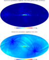 |
Fig. 10 Impact of spectral index uncertainty on the polarized intensity maps. Top: standard deviation of 50 maps obtained with βs drawn at random with a Gaussian distribution centered on βs = −3.1 and with a standard deviation of 0.1. Bottom: sum in quadrature of the above error and of the noise standard deviation. |
4.2 Comparison with other polarized synchrotron maps
Full-sky synchrotron polarization maps from Planck data alone have been obtained for the Planck 2018 data release using the SMICA (Delabrouille et al. 2003; Cardoso et al. 2008) and the Commander (Eriksen et al. 2004, 2008; Seljebotn et al. 2019) component separation pipelines (Planck Collaboration IV 2020). In both cases, however, only Planck data have been used, resulting in a noise penalty with respect to the composite polarized synchrotron polarization maps presented here. Our “Planck-revisited” maps are substantially better in terms of noise contamination and in terms of the characterization of the effective angular resolution. As all the data products are publicly available, we leave further comparison of our maps with those data products to the reader.
More interesting is the comparison with maps of the synchrotron amplitude and spectral index obtained from a combined analysis of Planck and WMAP data, which have recently been published by Watts et al. (2024), and which are also available for download on a dedicated website4.
Those synchrotron polarization Q and U maps are nominally produced at an angular resolution of 60′, but a prior smoothing of 30′ applied during the fitting, and an additional 1 degree smoothing added when taking the mean over the Gibbs chain, are susceptible to further degrading the effective angular resolution of the Cosmoglobe maps.
We estimated the Cosmoglobe maps’ angular resolution by computing the ratio
![Mathematical equation: $\[B_{\ell}^2=\frac{C_{\ell, 1 \times 2}^{\mathrm{CG}}}{C_{\ell}^{\mathrm{PR}}-N_{\ell}^{\mathrm{PR}}},\]$](/articles/aa/full_html/2024/09/aa50007-24/aa50007-24-eq5.png) (3)
(3)
where ![Mathematical equation: $\[C_{\ell, 1 \times 2}^{\mathrm{CG}}\]$](/articles/aa/full_html/2024/09/aa50007-24/aa50007-24-eq6.png) is the cross-spectrum of the HM1 and HM2 Cosmoglobe maps, and
is the cross-spectrum of the HM1 and HM2 Cosmoglobe maps, and ![Mathematical equation: $\[C_{\ell}^{\mathrm{PR}}-N_{\ell}^{\mathrm{PR}}\]$](/articles/aa/full_html/2024/09/aa50007-24/aa50007-24-eq7.png) is the noise-debiased auto-spectrum of our Planck-revisited map. The ratio, which is roughly compatible with an extra 30′ of smoothing in the Cosmoglobe maps, is displayed in Fig. 11 for the most interesting ℓ-range with respect to the detection of primordial CMB B-modes.
is the noise-debiased auto-spectrum of our Planck-revisited map. The ratio, which is roughly compatible with an extra 30′ of smoothing in the Cosmoglobe maps, is displayed in Fig. 11 for the most interesting ℓ-range with respect to the detection of primordial CMB B-modes.
The noise level in the total polarization amplitude,
![Mathematical equation: $\[\sigma_P=\sqrt{\sigma_Q^2+\sigma_U^2},\]$](/articles/aa/full_html/2024/09/aa50007-24/aa50007-24-eq8.png) (4)
(4)
is 3.4 μKrj in Cosmoglobe DR1. For comparison, the noise standard deviation obtained with the present analysis is about 2.78 μKrj at a resolution of 60′. When the map is further smoothed with a 30′ beam to match the Cosmoglobe map effective resolution determined above, this noise standard deviation reduces to 2.32 μKrj, 32% lower than that of the Cosmoglobe DR1 maps. The low noise contamination we achieve in the Planck-revisited synchrotron map is mostly due to efficient co-addition of the input maps across scales, pixels, and as a function of the Stokes parameter being considered, Q or U.
Power spectra for three different sky regions, corresponding to a low, medium, and high polarized synchrotron emission amplitude (using the masks displayed in Fig. 9), are shown in Fig. 12, together with power spectra computed from the Cosmoglobe DR1 data products. For each region, the mask selecting the level of contamination was apodized with a 2-degree cosine-squared transition, and point sources were masked using the mask shown in the bottom panel of Fig. 9, apodized with a 1-degree cosine-squared transition.
Overall, there is good agreement between the two data products at low ℓ. For intermediate ℓ, the Cosmoglobe synchrotron maps are noisier. At high ℓ, the overall power in the Cosmoglobe maps is lower, indicative of extra smoothing, as was already determined above.
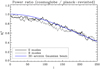 |
Fig. 11 Ratio of Cosmoglobe to Planck-revisited EE and BB power spectra over the region of sky with highest emission. |
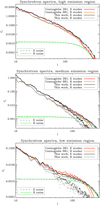 |
Fig. 12 Power spectra of polarized synchrotron emission in three different sky regions, selected using the masks outlined in Fig. 9. The data was plotted after smoothing the spectra with a Δℓ = 3 window. In the high- and medium-emission regions (top and middle panels), spectra are strongly signal-dominated. There is excellent agreement between our maps and the Cosmoglobe DR1 maps up to ℓ ≃ 30, above which the Cosmoglobe spectra are somewhat lower. At scales where signal dominates over noise, this discrepancy, increasing with increasing ℓ, must be due to different effective beams. In the low-emission region (bottom panel), of specific interest for future ground-based observations of CMB B-modes, the Cosmoglobe polarization maps have significantly higher power for 50 < ℓ < 100 than our maps. This is indicative of higher noise contamination, while the lower power of the Cosmoglobe maps at higher ℓ likely indicates a larger effective beam. For the medium- and low-contamination regions, we show the noise-debiased power spectra of our synchrotron polarization maps with “+” data points. Noise spectra were computed from 200 simulations of WMAP and Planck LFI noise, propagated through the analysis pipeline. |
4.3 Data products
“Planck-revisited” data products have been made available on a dedicated website5. Data products specific to this work comprise:
Maps of synchrotron Q and U Stokes parameters obtained with the method described in Sect. 3, at a resolution of 60′ (maps at a higher resolution can be made available by the author upon request).
Masks dividing the sky into three regions of different synchrotron polarized amplitudes (high, medium, and low polarized synchrotron emission).
A mask for strong polarized compact sources, which can be completed if necessary using the Planck catalog of nonthermal sources (Planck Collaboration Int. LIV 2018).
Maps of simulated noise for the 60′ resolution synchrotron Q and U polarization data products (additional simulations can be made available if necessary).
Maps of synchrotron polarization obtained with a randomized spectral index.
No attempt has been made to correct for residual systematics in the maps, or to fit for the scaling of synchrotron emission as a function of sky direction. For these reasons, caution must be used when exploiting our maps in regions of strong emission, where the calibration uncertainty due to scaling with frequency, as well as potential intensity to polarization leakage, can generate errors larger than the map noise. At very low ℓ (e.g., below ℓ = 20), systematics in the original data products are expected to project onto our synchrotron maps. However, in regions where the polarized synchrotron emission is low and for ℓ ranging from 20 to 100, our maps are the most accurate full-sky tracers of polarized synchrotron emission to date. In particular, they can be used as polarized synchrotron templates for upcoming searches, in low-foreground sky regions, of a recombination peak (around ℓ = 80) in CMB primordial B-modes. They can also usefully complement future CMB polarization observations from space such as those proposed with LiteBIRD or CORE (LiteBIRD Collaboration 2023; Delabrouille et al. 2018), whose frequency coverage does not extend to the lowest frequencies observed by WMAP and Planck.
5 Conclusion
In this paper, we have applied a simple yet effective pipeline to combine WMAP K, Ka, and Q maps and Planck LFI 30 GHz and 44 GHz maps into a single set of Q and U synchrotron polarization maps at 30 GHz. The effective angular resolution of the maps is that of a 60′ Gaussian beam, with a smooth cosine-square-shaped apodization from ℓ = 950 to ℓ = 1000. Additive errors from instrumental noise were evaluated with two hundred noise simulations propagated through the analysis pipeline. Multiplicative errors from the assumption of a uniform synchrotron emission law with βs = −3.1, evaluated with a Monte-Carlo pipeline over a distribution of spectral indices, are shown to be subdominant over most of the sky.
The maps and noise simulations have been made available to the scientific community on a dedicated data server, accessible from the web.
Acknowledgements
Some of the results in this paper have been derived using the HEALPix pixelization scheme (Górski et al. 2005). The author thanks Duncan Watts for useful discussions regarding comparison with the Cosmoglobe analysis and Cosmoglobe DR1 data products.
References
- Abazajian, K., Addison, G., Adshead, P., et al. 2019, arXiv e-prints [arXiv:1907.04473] [Google Scholar]
- Abbott, T. M. C., Aguena, M., Alarcon, A., et al. 2022, Phys. Rev. D, 105, 023520 [CrossRef] [Google Scholar]
- Ade, P., Aguirre, J., Ahmed, Z., et al. 2019, J. Cosmology Astropart. Phys., 2019, 056 [CrossRef] [Google Scholar]
- Alam, S., Ata, M., Bailey, S., et al. 2017, MNRAS, 470, 2617 [Google Scholar]
- Aurlien, R., Remazeilles, M., Belkner, S., et al. 2023, J. Cosmology Astropart. Phys., 2023, 034 [CrossRef] [Google Scholar]
- Bardeen, J. M., Steinhardt, P. J., & Turner, M. S. 1983, Phys. Rev. D, 28, 679 [Google Scholar]
- Basak, S., & Delabrouille, J. 2013, MNRAS, 435, 18 [Google Scholar]
- Bennett, C. L., Larson, D., Weiland, J. L., et al. 2013, ApJS, 208, 20 [Google Scholar]
- Benoît, A., Ade, P., Amblard, A., et al. 2003, A&A, 399, L19 [NASA ADS] [CrossRef] [EDP Sciences] [Google Scholar]
- Benoît, A., Ade, P., Amblard, A., et al. 2004, A&A, 424, 571 [NASA ADS] [CrossRef] [EDP Sciences] [Google Scholar]
- BICEP2 Collaboration, Keck Array Collaboration, Ade, P. A. R., et al. 2016, Phys. Rev. Lett., 116, 031302 [NASA ADS] [CrossRef] [Google Scholar]
- BICEP/Keck Collaboration 2022, arXiv e-prints [arXiv:2203.16556] [Google Scholar]
- Cardoso, J.-F., Le Jeune, M., Delabrouille, J., Betoule, M., & Patanchon, G. 2008, IEEE J. Selected Topics Signal Process., 2, 735 [NASA ADS] [CrossRef] [Google Scholar]
- Das, S., Louis, T., Nolta, M. R., et al. 2014, J. Cosmology Astropart. Phys., 2014, 014 [CrossRef] [Google Scholar]
- Davis, Leverett, J., & Greenstein, J. L. 1951, ApJ, 114, 206 [NASA ADS] [CrossRef] [Google Scholar]
- de Belsunce, R., Gratton, S., & Efstathiou, G. 2022, MNRAS, 517, 2855 [NASA ADS] [CrossRef] [Google Scholar]
- Delabrouille, J., Cardoso, J. F., & Patanchon, G. 2003, MNRAS, 346, 1089 [NASA ADS] [CrossRef] [Google Scholar]
- Delabrouille, J., Betoule, M., Melin, J. B., et al. 2013, A&A, 553, A96 [NASA ADS] [CrossRef] [EDP Sciences] [Google Scholar]
- Delabrouille, J., de Bernardis, P., Bouchet, F. R., et al. 2018, J. Cosmology Astropart. Phys., 2018, 014 [CrossRef] [Google Scholar]
- de la Hoz, E., Barreiro, R. B., Vielva, P., et al. 2023, MNRAS, 519, 3504 [NASA ADS] [CrossRef] [Google Scholar]
- Eisenstein, D. J., Zehavi, I., Hogg, D. W., et al. 2005, ApJ, 633, 560 [Google Scholar]
- Eriksen, H. K., O’Dwyer, I. J., Jewell, J. B., et al. 2004, ApJS, 155, 227 [Google Scholar]
- Eriksen, H. K., Jewell, J. B., Dickinson, C., et al. 2008, ApJ, 676, 10 [Google Scholar]
- Errard, J., Remazeilles, M., Aumont, J., et al. 2022, ApJ, 940, 68 [NASA ADS] [CrossRef] [Google Scholar]
- Fuskeland, U., Andersen, K. J., Aurlien, R., et al. 2021, A&A, 646, A69 [NASA ADS] [CrossRef] [EDP Sciences] [Google Scholar]
- Górski, K. M., Hivon, E., Banday, A. J., et al. 2005, ApJ, 622, 759 [Google Scholar]
- Hanany, S., Ade, P., Balbi, A., et al. 2000, ApJ, 545, L5 [Google Scholar]
- Hanany, S., Alvarez, M., Artis, E., et al. 2019, arXiv e-prints [arXiv:1902.10541] [Google Scholar]
- Henning, J. W., Sayre, J. T., Reichardt, C. L., et al. 2018, ApJ, 852, 97 [Google Scholar]
- Hui, H., Ade, P. A. R., Ahmed, Z., et al. 2018, SPIE Conf. Ser., 10708, 1070807 [Google Scholar]
- Kamionkowski, M., & Kovetz, E. D. 2016, ARA&A, 54, 227 [NASA ADS] [CrossRef] [Google Scholar]
- Kogut, A., Dunkley, J., Bennett, C. L., et al. 2007, ApJ, 665, 355 [Google Scholar]
- Krachmalnicoff, N., Carretti, E., Baccigalupi, C., et al. 2018, A&A, 618, A166 [NASA ADS] [CrossRef] [EDP Sciences] [Google Scholar]
- LiteBIRD Collaboration (Allys, E., et al.) 2023, Prog. Theor. Exp. Phys., 2023, 042F01 [CrossRef] [Google Scholar]
- Louis, T., Grace, E., Hasselfield, M., et al. 2017, J. Cosmology Astropart. Phys., 2017, 031 [CrossRef] [Google Scholar]
- Martin, J., Ringeval, C., & Vennin, V. 2014, Phys. Dark Universe, 5, 75 [CrossRef] [Google Scholar]
- Mather, J. C., Cheng, E. S., Cottingham, D. A., et al. 1994, ApJ, 420, 439 [Google Scholar]
- Netterfield, C. B., Ade, P. A. R., Bock, J. J., et al. 2002, ApJ, 571, 604 [NASA ADS] [CrossRef] [Google Scholar]
- Perlmutter, S., Aldering, G., Goldhaber, G., et al. 1999, ApJ, 517, 565 [Google Scholar]
- Planck Collaboration IX. 2016, A&A, 594, A9 [NASA ADS] [CrossRef] [EDP Sciences] [Google Scholar]
- Planck Collaboration I. 2020, A&A, 641, A1 [NASA ADS] [CrossRef] [EDP Sciences] [Google Scholar]
- Planck Collaboration IV. 2020, A&A, 641, A4 [NASA ADS] [CrossRef] [EDP Sciences] [Google Scholar]
- Planck Collaboration XI. 2020, A&A, 641, A11 [NASA ADS] [CrossRef] [EDP Sciences] [Google Scholar]
- Planck Collaboration Int. LIV. 2018, A&A, 619, A94 [NASA ADS] [CrossRef] [EDP Sciences] [Google Scholar]
- Planck Collaboration Int. LVII. 2020, A&A, 643, A42 [NASA ADS] [CrossRef] [EDP Sciences] [Google Scholar]
- POLARBEAR Collaboration (Ade, P. A. R., et al.) 2017, ApJ, 848, 121 [Google Scholar]
- Salatino, M., Austermann, J., Thompson, K. L., et al. 2020, SPIE Conf. Ser., 11453, 114532A [Google Scholar]
- Schillaci, A., Ade, P. A. R., Ahmed, Z., et al. 2020, J. Low Temp. Phys., 199, 976 [NASA ADS] [CrossRef] [Google Scholar]
- Seljebotn, D. S., Bærland, T., Eriksen, H. K., Mardal, K. A., & Wehus, I. K. 2019, A&A, 627, A98 [NASA ADS] [CrossRef] [EDP Sciences] [Google Scholar]
- Smoot, G. F., Bennett, C. L., Kogut, A., et al. 1992, ApJ, 396, L1 [Google Scholar]
- Thorne, B., Dunkley, J., Alonso, D., & Næss, S. 2017, MNRAS, 469, 2821 [Google Scholar]
- Tristram, M., Banday, A. J., Górski, K. M., et al. 2022, Phys. Rev. D, 105, 083524 [Google Scholar]
- Watts, D. J., Fuskeland, U., Aurlien, R., et al. 2024, A&A, 686, A297 [NASA ADS] [CrossRef] [EDP Sciences] [Google Scholar]
- Weiland, J. L., Addison, G. E., Bennett, C. L., Halpern, M., & Hinshaw, G. 2022, ApJ, 936, 24 [NASA ADS] [CrossRef] [Google Scholar]
- Zonca, A., Thorne, B., Krachmalnicoff, N., & Borrill, J. 2021, J. Open Source Softw., 6, 3783 [NASA ADS] [CrossRef] [Google Scholar]
Those maps can be made available upon request, but are not part of the default data products made available with this paper.
Residuals are small, and for most uses can be safely neglected. In case of doubt, contact the author.
All Tables
All Figures
|
Fig. 1 Noise standard deviation maps for the three WMAP channels used in this work (K, Ka and Q), rescaled to equivalent 30 GHz noise assuming a synchrotron spectral index of −3.1. Units are in μKcmb. Each map displays the average of the standard deviation of the Q and U Stokes parameter maps. |
| In the text | |
|
Fig. 2 Noise standard deviation maps for the two Planck LFI channels used in this work (30 and 44 GHz), rescaled to equivalent 30 GHz noise assuming a synchrotron spectral index of −3.1. Units are in μKcmb. Each map displays the average of the standard deviation of the Q and U Stokes parameter maps. Here and in Fig. 1, different color scales have been used for the different frequency channels. We note that the noise level for each channel is variable across the sky, and that the shape and location of the lowest-noise regions is channel-dependent. The map depth varies by an order of magnitude across the sky, and the lowest-noise regions are different between the maps. This calls for pixel-dependent weights for map combination. |
| In the text | |
|
Fig. 3 Beam-corrected noise spectra for the WMAP and Planck channels used in this work, rescaled to equivalent 30 GHz noise assuming a synchrotron spectral index of −3.1. The relative sensitivity of the different channels strongly depends on the harmonic scale, ℓ. On the largest scales, the WMAP K band and the LFI 30 GHz channels have a comparable mean synchrotron sensitivity (with, however, a strong pixel dependence, as is seen in Figs. 1 and 2. At ℓ ≃ 800, however, the WMAP Q and LFI 44 GHz are about as sensitive as the LFI 30 GHz channel, and much more sensitive than the WMAP K band. |
| In the text | |
|
Fig. 4 Cosine-shaped needlet bands, hJ(ℓ), used in this work. As usual, those are normalized so that ∑J hJ(ℓ)2 = 1 for a useful range of ℓ. Here, this normalization holds up to ℓ = 950. For higher ℓ, the sum goes smoothly to zero at ℓmax = 1000 with a cosine-square half-arch. |
| In the text | |
|
Fig. 5 Weights used for the reconstruction of the synchrotron Q (top two) and U (bottom two) synchrotron polarization maps in the first needlet band. Only the weights of the WMAP K and the Planck LFI 30 GHz maps are shown, as only those are significant for that scale (and add up to almost one). We note the differences between Q and U weights. |
| In the text | |
|
Fig. 6 Stokes Q (top) and U (bottom) 30 GHz polarization maps obtained with the pipeline described in this paper, at an angular resolution of 1 degree. |
| In the text | |
|
Fig. 7 Beam-corrected noise spectra for the WMAP and Planck channels used in this work, rescaled to equivalent 30 GHz noise assuming a synchrotron spectral index of −3.1, as in Fig. 3. An extra black curve shows the noise spectrum of the final composite synchrotron map obtained in this work, which near-optimally combines all observations. |
| In the text | |
|
Fig. 8 Synchrotron and noise polarized intensity obtained in this work. Top: total polarized intensity, |
| In the text | |
|
Fig. 9 Masks used to compute power spectra shown in Fig. 12. In the top panel, the low, medium, and high-amplitude regions of emission are shown in black, dark gray, and light gray, respectively. The white region, located in the inner Galactic ridge, corresponds to the strongest region of polarized synchrotron emission, and is excluded for all power spectra computations. The bottom panel shows a mask for compact sources. |
| In the text | |
|
Fig. 10 Impact of spectral index uncertainty on the polarized intensity maps. Top: standard deviation of 50 maps obtained with βs drawn at random with a Gaussian distribution centered on βs = −3.1 and with a standard deviation of 0.1. Bottom: sum in quadrature of the above error and of the noise standard deviation. |
| In the text | |
|
Fig. 11 Ratio of Cosmoglobe to Planck-revisited EE and BB power spectra over the region of sky with highest emission. |
| In the text | |
|
Fig. 12 Power spectra of polarized synchrotron emission in three different sky regions, selected using the masks outlined in Fig. 9. The data was plotted after smoothing the spectra with a Δℓ = 3 window. In the high- and medium-emission regions (top and middle panels), spectra are strongly signal-dominated. There is excellent agreement between our maps and the Cosmoglobe DR1 maps up to ℓ ≃ 30, above which the Cosmoglobe spectra are somewhat lower. At scales where signal dominates over noise, this discrepancy, increasing with increasing ℓ, must be due to different effective beams. In the low-emission region (bottom panel), of specific interest for future ground-based observations of CMB B-modes, the Cosmoglobe polarization maps have significantly higher power for 50 < ℓ < 100 than our maps. This is indicative of higher noise contamination, while the lower power of the Cosmoglobe maps at higher ℓ likely indicates a larger effective beam. For the medium- and low-contamination regions, we show the noise-debiased power spectra of our synchrotron polarization maps with “+” data points. Noise spectra were computed from 200 simulations of WMAP and Planck LFI noise, propagated through the analysis pipeline. |
| In the text | |
Current usage metrics show cumulative count of Article Views (full-text article views including HTML views, PDF and ePub downloads, according to the available data) and Abstracts Views on Vision4Press platform.
Data correspond to usage on the plateform after 2015. The current usage metrics is available 48-96 hours after online publication and is updated daily on week days.
Initial download of the metrics may take a while.