| Issue |
A&A
Volume 689, September 2024
|
|
|---|---|---|
| Article Number | A149 | |
| Number of page(s) | 17 | |
| Section | Stellar structure and evolution | |
| DOI | https://doi.org/10.1051/0004-6361/202449634 | |
| Published online | 09 September 2024 | |
The impact of asteroseismically calibrated internal mixing on nucleosynthetic wind yields of massive stars
1
Institute of Astronomy, KU Leuven, Celestijnenlaan 200D, 3001 Leuven, Belgium
2
Konkoly Observatory, Research Centre for Astronomy and Earth Sciences, HUN-REN, Konkoly Thege Miklós út 15-17, 1121 Budapest, Hungary
3
CSFK, MTA Centre of Excellence, Konkoly Thege Miklós út 15-17, 1121 Budapest, Hungary
4
INAF – Osservatorio Astronomico di Roma, Via Frascati 33, 00040 Monteporzio Catone, Italy
5
Department of Astrophysics, IMAPP, Radboud University Nijmegen, PO Box 9010, 6500 GL Nijmegen, The Netherlands
6
Max Planck Institute for Astronomy, Königstuhl 17, 69117 Heidelberg, Germany
Received:
16
February
2024
Accepted:
19
June
2024
Abstract
Context. Asteroseismology gives us the opportunity to look inside stars and determine their internal properties, such as the radius and mass of the convective core. Based on these observations, estimations can be made for the amount of the convective boundary mixing and envelope mixing of such stars and for the shape of the mixing profile in the envelope. However, these results are not typically included in stellar evolution models.
Aims. We aim to investigate the impact of varying convective boundary mixing and envelope mixing in a range based on asteroseismic modelling in stellar models up to the core collapse, both for the stellar structure and for the nucleosynthetic yields. In this first study, we focus on the pre-explosive evolution and we evolved the models to the final phases of carbon burning. This set of models is the first to implement envelope mixing based on internal gravity waves for the entire evolution of the star.
Methods. We used the MESA stellar evolution code to simulate stellar models with an initial mass of 20 M⊙ from zero-age main sequence up to a central core temperature of 109 K, which corresponds to the final phases of carbon burning. We varied the convective boundary mixing, implemented as ‘step-overshoot’, with the overshoot parameter (αov) in the range 0.05−0.4. We varied the amount of envelope mixing (log(Denv/cm2 s−1)) in the range 0−6 with a mixing profile based on internal gravity waves. To study the nucleosynthesis taking place in these stars in great detail, we used a large nuclear network of 212 isotopes from 1H to 66Zn.
Results. Enhanced mixing according to the asteroseismology of main-sequence stars, both at the convective core boundary and in the envelope, has significant effects on the nucleosynthetic wind yields. This is especially the case for 36Cl and 41Ca, whose wind yields increase by ten orders of magnitude compared to those of the models without enhance envelope mixing. Our evolutionary models beyond the main sequence diverge in yields from models based on rotational mixing, having longer helium-burning lifetimes and lighter helium-depleted cores.
Conclusions. We find that the asteroseismic ranges of internal mixing calibrated from core hydrogen-burning stars lead to similar wind yields as those resulting from the theory of rotational mixing. Adopting the seismic mixing levels beyond the main sequence, we find earlier transitions to radiative carbon burning compared to models based on rotational mixing because they have lower envelope mixing in that phase. This influences the compactness and the occurrence of shell mergers, which may affect the supernova properties and explosive nucleosynthesis.
Key words: asteroseismology / nuclear reactions / nucleosynthesis / abundances / stars: evolution / stars: interiors / stars: massive / stars: winds / outflows
Corresponding author; This email address is being protected from spambots. You need JavaScript enabled to view it. .
© The Authors 2024
 Open Access article, published by EDP Sciences, under the terms of the Creative Commons Attribution License (https://creativecommons.org/licenses/by/4.0), which permits unrestricted use, distribution, and reproduction in any medium, provided the original work is properly cited.
This article is published in open access under the Subscribe to Open model. This email address is being protected from spambots. You need JavaScript enabled to view it. to support open access publication.
1. Introduction
Massive stars (M* ≥ 10 M⊙, in this context) are one of the main sources of nucleosynthesis in the Universe (see, e.g. Hirschi et al. 2005; Ekström et al. 2012; Pignatari et al. 2016; Ritter et al. 2018; Limongi & Chieffi 2018, and many others). During their lives and deaths, they turn the lighter elements into heavier ones. The nucleosynthetic yields of these stars, aside from the initial mass and initial metallicity, depend on three main ingredients: (i) the nuclear reaction rates, which govern the production and destruction of isotopes inside the star (see, e.g. Kobayashi et al. 2020; ii) the internal mixing, which is responsible for moving the isotopes from where they are produced to other layers of the star (Pedersen et al. 2021); and (iii) mass loss, through stellar winds (Kudritzki & Puls 2000; Langer 2012; Smith 2014), supernova explosions (including the explosion mechanism and the isotopes produced during the explosive nucleosynthesis) (Woosley et al. 2002; Nomoto et al. 2013), and binary interactions (Sana et al. 2012), which expel the isotopes into the interstellar medium. In this work, we focus on the effects of internal mixing on the nucleosynthetic wind yields, while we maintained the nuclear reaction rates and the mass-loss rates at standard values and we did not consider the supernova explosion. We did this because even though the internal mixing is very important for the wind yields, it is currently not well constrained. The internal mixing near the convective core during the main sequence is important because it impacts the mass of the hydrogen-depleted core at the end of this stage, setting the stage for the nuclear burning in the more evolved stages (Johnston 2021; Pedersen 2022) and how much of the burning products reach the surface of the star from where they are expelled.
The main mixing mechanism for massive stars is convective mixing. It transports both the nuclear energy produced in the burning zones (either the stellar core or burning shells), as well as the isotopes produced in these areas. However, since convection is a 3D process (while stellar evolution on nuclear timescales can only be handled in 1D), it can only be modelled by a parametric approach. Aside from the choice between the Ledoux or Schwarzschild criterion for convection, it needs to be taken into account that the convective motions do not stop at the boundaries of such zones. Convective boundary mixing (CBM hereafter) is needed to correct for this and with the introduction of a treatment of CBM, free parameters are also introduced. Commonly these parameters are either fov or αov (with a mapping factor of αov/fov ∼ 10, see, e.g. Kaiser et al. 2020, Sect. 3.1). We note that fov is linked to exponential overshoot, where the CBM is treated via an exponential decay of the convective diffusion coefficient beyond the convective boundary as given in Herwig et al. (1997):
 (1)
(1)
Here, the diffusion coefficient, Dov, is a function of the distance from the convective boundary, the free parameter, fov, and the pressure scale height, Hp, at the convective boundary. We note that D0 is the value of the diffusion coefficient determined from the mixing length theory (Böhm-Vitense 1958). In this prescription for the CBM, the thermal structure in the mixing zone is that of the envelope, such that ∇T = ∇rad (Herwig 2000). Furthermore, αov is linked to convective penetration, also known as ‘step-overshoot’, which completely mixes the region with a distance l above the convective boundary given by:
 (2)
(2)
Here the thermal structure in the mixing zone is that of the core, such that ∇T = ∇ad (Zahn 1991). Many different studies have attempted to constrain these free parameters, leading to a wide range of possible values, ranging from αov = 0.0 (Wu et al. 2020) to 1.5 (Guenther et al. 2014), depending on the initial mass of the star and whether the effects of rotational mixing were included in the stellar models.
Asteroseismology gives us a way to look inside stars and determine the size and mass of their convective cores (see, e.g. Aerts et al. 2003; Dupret et al. 2004; Straka et al. 2005; Briquet et al. 2007, 2012; Montalbán et al. 2013; Moravveji et al. 2015; Deheuvels et al. 2016; Mombarg et al. 2019; Angelou et al. 2020; Viani & Basu 2020; Noll et al. 2021; Pedersen et al. 2021; Burssens et al. 2023). These studies, in which the stars do not rotate or rotate at a negligible velocity (at most ∼5% of their critical rotational velocity on the main sequence), revealed that in addition to the enhanced CBM (αov > 0), mixing in the envelope needs to be included to match asteroseismic observables. Moreover, period-spacing patterns caused by internal gravity waves detected in light curves of fast rotators reveal that the size of the convective core and the shape of the chemical gradient on the main sequence are different from what has been calculated from most grids of stellar evolution models (Aerts 2021). This leads to the conclusion that the treatment of internal mixing in stellar models needs to be adjusted to bring the models closer to what is observed (Johnston 2021). Similar results are found by other studies, such as Tkachenko et al. (2020), based on detached binary systems on the main sequence rather than pulsating stars.
Kaiser et al. (2020) did a theoretical study on the effect of the relative importance of convective uncertainties in massive stars, focusing on CBM and the strength of semi-convection. The authors present the stellar structure of models during hydrogen and helium burning, for stars with initial masses of 15, 20, and 25 M⊙. Kaiser et al. (2020) show that the amount of CBM considered in their models affects the duration of the burning phases, the surface evolution of the stars, the size of the convective cores, but also the isotopic mixture in the core. This has implications for the 12C/16O ratio at the end of core helium burning, which impacts the explosive nucleosynthesis, and thus the supernova yields.
In this work, we focus on models with an initial mass of 20 M⊙, from the main sequence up to a central temperature of 1 GK. This mass is chosen because the structure of this star on the main sequence is comparable to one of the most massive gravity-mode pulsators available in asteroseismic studies (Pedersen et al. 2021; Pedersen 2022). These pulsators have a convective core and radiative envelope on the main sequence. The determined amount of CBM and envelope mixing, as well as the mixing profile, is similar for stars in the mass range without a strong wind. A 20 M⊙ star is interesting because the star does not undergo strong mass loss during the main sequence and is expected to explode in a Type-II supernova explosion (see, e.g. Woosley et al. 2002; Sukhbold et al. 2016; Limongi & Chieffi 2018). We study the impact of CBM and envelope mixing on the nucleosynthetic wind yields. Also, a 20 M⊙ model is often used in grids of massive stars from various codes, which allows for comparison studies. We vary the CBM and the envelope mixing within the range of values found for αov and log(Denv/cm2 s−1) by Pedersen et al. (2021), Pedersen (2022) (see Table 2 in the latter work). The models are calculated up to a central temperature of 1 GK to determine the effects on the evolution of the star and on the nucleosynthetic yields.
The paper is structured as follows; in Section 2 we describe the physical input for the models and justify the choices made. In Section 3 we describe the effects of changing the internal mixing on the stellar evolution, with particular attention to the resulting core composition. In Section 4 we discuss the surface abundances and the stellar yields. We finish with a discussion and conclusions in Section 5.
2. Method and input physics
We have used the MESA (Modules for Experiments in Astrophysics) stellar evolution code version 22.11.1 (Paxton et al. 2011, 2013, 2015, 2018, 2019; Jermyn et al. 2023) for the simulations presented in this paper.
2.1. Nuclear physics input
We made use of the JINA Reaclib (Cyburt et al. 2010). In the latest revisions of MESA, the default reaction rates are set to NACRE (Angulo et al. 1999), unless not available. The NACRE compilation consists of 86 reaction rates, of which 32 are also contained in the JINA Reaclib. The other 54 rates were replaced by their updated rates as given in version 2.2 of the JINA Reaclib by manually including the tables into MESA. This includes the updated 14N(p,γ)15O by Imbriani et al. (2005). This rate has a strong impact on the main-sequence evolution of stars undergoing hydrogen burning via the CNO cycle.
The initial mass of the all models presented here is 20 M⊙. We used an initial metallicity of Z = 0.014 combined with the isotopic mixture as given by Przybilla et al. (2013). The initial hydrogen content is then defined as Xini = 1 − Yini − Zini. The initial helium content is determined as follows; Yini = 0.2465+2.1 × Zini, where the value of 0.2465 refers to the primordial helium abundance as determined by Aver et al. (2013). The value of 2.1 is chosen such that the mass fractions of the chemical mixture adopted from Przybilla et al. (2013) are reproduced (see also Michielsen et al. 2021). Our nuclear network contained all the relevant isotopes for the main burning phases (H, He, C, Ne, O, and Si), allowing us to follow the evolution of the stars in detail up to core collapse. Including the ground and isomeric states of 26Al, the total nuclear network contains the following 212 isotopes: n, 1 − 3H, 3, 4He, 6, 7Li, 7 − 10Be, 8 − 11B, 11 − 14C, 13 − 16N, 14 − 19O, 17 − 20F, 19 − 23Ne, 21 − 24Na, 23 − 27 Mg, 25Al, 26Alg, 26Alm, 27, 28Al, 27 − 33Si, 29 − 34P, 31 − 37S, 35 − 38Cl, 35 − 41Ar, 39 − 44K, 39 − 49Ca, 43 − 51Sc, 43 − 54Ti, 47 − 58V, 47 − 58Cr, 51 − 59Mn, 51 − 66Fe, 55 − 67Co, 55 − 69Ni, 59 − 66Cu, and 59 − 66Zn. This network includes all 204 isotopes that influence the final value of the electron fraction, Ye (see, e.g. Farmer et al. 2016, and references therein), which affects the supernova properties (see Heger et al. 2000).
2.2. Selection of the mixing parameters
We made use of the Ledoux criterion to establish the location of the convective boundaries. Convection itself was treated according to the MLT++ prescription (Paxton et al. 2013). This prescription introduced a free parameter, αmlt. Here we set αmlt to 2 for all phases of the evolution.
The semi-convection parameter, αsc, was set to 0.01 for the entire evolution. Especially for the models with a large amount of CBM, the impact of αsc is limited (see, e.g. Kaiser et al. 2020). The thermohaline coefficient, αtherm, was set to 1 for hydrogen and helium burning and to 0 beyond helium burning to reduce the complexity of the models.
2.2.1. Convective boundary mixing
For the main sequence, we made use of the CBM scheme as implemented by Michielsen et al. (2019). This scheme allows for a combination of the two CBM schemes mentioned in the introduction, ‘exponential’ and ‘step’ overshoot. In the present work, however, we only considered the so-called ‘step overshoot’ part of this scheme (also referred to as convective penetration), since most of the B stars analysed by Pedersen (2022) favour this variant for the CBM (55% versus 45% for the “exponential overshoot or diffusive exponentially decaying overshooting”). We varied the CBM, here parameterised by αov, based on the asteroseismic estimates by Pedersen et al. (2021, Pedersen (2022). For the values for the overshoot parameter, αov, we took the upper limit for the most massive stars in the sample following the profile where the envelope mixing is governed by internal gravity waves (noted by ψ2, 6 in Pedersen 2022) either as the most likely candidate or the second most likely candidate, as indicated in Table 6 of Pedersen (2022). The models with ψ2 favour the ‘exponential overshoot’ scheme and for these cases we used a conversion factor of ∼10 from the exponential overshoot parameter, fov, to compute the level of the step overshoot parameter such stars would have. This might be a slight underestimation of the conversion, as Claret & Torres (2017) find a factor of αov/fov = 11.36 ± 0.22, Moravveji et al. (2016) find a factor of 13, and Valle et al. (2017) a factor of 12. Based on a conversion of 10, αov is varied between 0.05−0.4 on the main sequence, with f0 = 0.005. The parameter f0 determines the location inside the convective core from where the CBM starts, which is for computational reasons. This would also be the case for the exponential overshoot scheme (see, e.g. Kaiser et al. 2020, Sect. 3.1).
Little is known about the more evolved stages of massive stars from asteroseismology. Therefore, we looked at subdwarf B stars, low mass core-helium burning stars, for guidance. These stars have convective helium-burning cores surrounded by a thin envelope, making their structure similar to that of an evolved massive star, and they are suitable for asteroseismology. Seismic studies of these stars (see, e.g. Van Grootel et al. 2010a,b; Charpinet et al. 2010, 2011; Ghasemi et al. 2017; Uzundag et al. 2021), reveal that during the core helium burning stage of these stars additional CBM is necessary to explain the observations. Few pulsating subdwarfs have been modelled, however. Therefore we used a typical amount of CBM with αov = 0.2 for this evolutionary phase and beyond for the convective cores. For hydrogen shell-burning, we again made use of CBM via the ‘step-overshoot’ scheme with αov = 0.20 and f0 = 0.005. We did not use CBM for any of the later burning shells aside from the hydrogen-burning shell.
2.2.2. Enhanced envelope mixing
Aside from the mixing at the convective boundaries, there is also mixing in the envelopes of a massive star. Extra mixing in the envelope is needed for the stellar evolution models to match the asteroseismic observations. In Pedersen et al. (2021) four different profiles for the envelope mixing are implemented for the asteroseismic modelling; a flat profile leading to a constant envelope mixing, a profile based on hydrodynamic simulations of internal gravity waves (Rogers & McElwaine 2017; Varghese et al. 2023), a profile where the mixing is due to vertical shear (Mathis et al. 2004), and lastly a profile where the mixing is due to meridional circulation caused by rotation combined with vertical shear (Georgy et al. 2013). In this work we focused on the profile driven by internal gravity waves because this profile has so far not been used in the global investigation of internal mixing despite that it has been shown to explain asteroseismic data well. Also, this profile has not been investigated beyond the main sequence. The first profile used by Pedersen et al. (2021) cannot satisfactorily reproduce the seismic properties of their sample and the latter two profiles both are based on the effects of stellar rotation, which have already been extensively investigated in the literature as there are many rotating models available calculated with various codes and implementations (see, e.g. Heger et al. 2000; Ekström et al. 2008, 2012; Chieffi & Limongi 2013; Limongi & Chieffi 2018; Banerjee et al. 2019; Brinkman et al. 2021; Brinkman 2022). For the implementation of the mixing profile based on internal gravity waves, we followed the implementation of Michielsen et al. (2021). Here the mixing profile is determined as DIGW(r) = Denv(ρ(rCBM)/ρ(r)), where Denv is the free parameter and determines the strength of the mixing at the connection point between the extended CBM region and the envelope, ρ(rCBM) being the density at the border between the CBM region and the envelope, and ρ(r) is the local density. The value of log(Denv/cm2 s−1) was varied between 0−6 in steps of 1.5, based on the results by Pedersen et al. (2021), Pedersen (2022). We took the values for log(Denv/cm2 s−1) from the same models we previously selected for αov.
To determine the location of the convective boundary in the models with limited CBM (αov = 0.05 and 0.1), we implemented the convective premixing scheme as described in Paxton et al. (2019) on the main sequence. For this, we enhanced the mesh locally around the convective boundary of the hydrogen burning core.
The profile based on internal gravity waves was originally created for the main sequence (Michielsen et al. 2021). Here we also applied it to the rest of the stellar evolution, most importantly to helium burning. The other burning phases are relatively short and the diffusive mixing is not fast enough to be of significant impact. During helium burning, however, the star has a convective core, which can drive internal gravity waves and thus induce mixing. In the previously mentioned works on subdwarf B stars, no mention is made of enhanced envelope mixing. However, based on the stellar structure, we assumed here that the convective helium burning core can drive internal gravity waves as well and we used the same profile as on the main sequence. The continued enhanced envelope mixing is an important difference from models that consider stellar rotation, since at this point in the evolution, the stellar rotation of the envelope has reduced significantly (see, e.g. Aerts et al. 2019) and its impact on the interior mixing should therefore be diminished.
2.3. Other input
The mass-loss scheme is a combination of three different wind prescriptions. For the hot phase (Teff ≥ 11 kK), we used the prescription given by Vink et al. (2000, 2001), which has been divided by 3 to match the rates of Björklund et al. (2021). For the cold phase (Teff ≤ 1 kK) we used Nieuwenhuijzen & de Jager (1990). For the stars that reach the WR-phase (Xsurf ≤ 0.4) we used the rates by Nugis & Lamers (2000). All phases of the wind have a metallicity dependence Ṁ ∝ Z0.85 following Vink et al. (2000) and Vink & de Koter (2005).
We have evolved the stars to a central temperature of 109 K, which, depending on the model, is during or after carbon burning. At this point, the mass loss is finished and the wind contribution to the nucleosynthetic yields can be calculated.
2.4. Yield calculation
Since our focus is on the pre-supernova nucleosynthetic yields from the winds, we calculated them as follows; we integrated over time the surface mass fraction multiplied by the mass loss. This gave us the total yield of the stellar model. For the stable isotopes, there is a second yield to consider, the net yield, that is, the total yield minus the initial total mass of the isotope originally present in the star. For short-lived radioactive isotopes the net yield is identical to the total yield, because the initial mass present in the stars is zero for these isotopes and thus no distinction is made for these yields. Hereafter, the yield always refers to the total wind yield, unless otherwise indicated.
3. Stellar models: Results and discussion
In this section, we discuss the results of our stellar evolution models in terms of evolutionary properties. Table A.1 contains the key information about the evolutionary stages.
3.1. Impact of enhanced mixing on the stellar evolution
On the main sequence, both the effects of envelope mixing by internal gravity waves and a larger amount of CBM are comparable to the effects of rotational induced mixing. The main-sequence lifetime is extended by increasing values of both αov and log(Denv/cm2 s−1) (see left panel of Fig. 1). Also, the main-sequence turnoff moves to a higher luminosity and effective temperature, as can be seen in the right panel of Fig. 2. This effect is the strongest for log(Denv/cm2 s−1) = 6, while for the other values of log(Denv/cm2 s−1) the effect is minimal. These results are in line with the literature for rotational mixing (see, e.g. Hirschi et al. 2004; Ekström et al. 2012; Limongi & Chieffi 2018, and the grey lines in the right panel of Fig. 2) and for enhanced CBM (see, e.g. Kaiser et al. 2020). A comparison of rotating versus non-rotating models can be found in, for example Brinkman et al. (2021). In Fig. 2 the grey lines show the results of that work, with the model without rotation overlapping mostly with our model with αov = 0.2 and log(Denv/cm2 s−1) = 0. On the evolutionary track, our model with log(Denv/cm2 s−1) = 6 shows a lot of similarities with the model rotating at 300 km/s (see right panel of Fig. 2). Both models have a higher luminosity at the end of the main sequence compared to the other models and experience more mass loss as well. Both enhanced envelope mixing and enhanced CBM lead to a larger amount of mass loss on the main sequence.
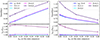 |
Fig. 1. Duration of core hydrogen burning (tH, left panel) and core helium burning (tHe, right panel) as a function of αov. To highlight the differences, the bottom panels show the ratio between models without additional envelope mixing (reference, in blue) and the other models with the same αov on the main sequence. |
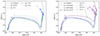 |
Fig. 2. Tracks in the Hertzsprung-Russel diagram for the different values of αov and no extra envelope mixing (log(Denv/cm2 s−1) = 0) (left panel) and for the different values of log(Denv/cm2 s−1) for a fixed value of αov = 0.2 (right panel). The different colours indicate the different values for the CBM and the envelope mixing. In the left panel, the grey line shows the non-rotating model from Brinkman et al. (2021) with αov = 0.2. In the right panel, the rotating models with initial rotational velocities for 150 and 300 km/s are added as a comparison for the different treatment of envelope mixing. The blue line is the same model in both panels. Only the model with log(Denv/cm2 s−1) = 6 shows a significant difference from the other models with the same amount of CBM, while even a moderately different αov produces a discernible shift. |
After the main sequence, the models with the only enhanced CBM but without enhanced envelope mixing behave comparably to models with rotational mixing, which have shorter helium burning lifetimes compared to their non-rotating counterparts (see right panel of Fig. 1). All our models from this point have the same amount of CBM and all differences propagate from differences caused by their the main sequence evolution. This has an analogue with rotational mixing, which loses its efficiency as the rotational velocity of the envelope slows down after the main sequence (Aerts et al. 2019).
The models with enhanced envelope mixing are dissimilar from rotating stellar models in the literature and ours without such mixing. The envelope mixing profile based on internal gravity waves requires the existence of a convective core in massive stars, which is still present during the advanced burning stages (except in a few cases where the models undergo radiative carbon burning rather than convective carbon burning, see below). This in principle allows for continued mixing between the envelope and the core as we consider it here. The enhanced mixing affects the size of the helium burning core. At the end of the main sequence the helium cores, hereafter referred as hydrogen-depleted cores to avoid confusion with the helium burning-core, are larger for models with increasing amounts of envelope mixing (see left panel of Fig. 3), which is due to an influx of fresh hydrogen from the stellar envelope, not dissimilar to what is happening for models that include rotational mixing.
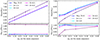 |
Fig. 3. Mass of the stellar cores at the end of hydrogen burning (left panel) and helium burning (right panel) as a function of the overshoot parameter. The lower panels show the ratio between the models with no extra envelope mixing and the other models with the overshoot parameter. |
At the onset of helium burning, the models with enhanced envelope mixing, log(Denv/cm2 s−1) = 6.0, have a larger convective core as expected based on the size of their larger hydrogen-depleted cores (see left panel of Fig. 3). However, as helium burning proceeds, the convective core region grows less in mass than for the models without enhanced mixing. This is due to the continued influx of helium from the region just above the helium burning core, which then leads to smaller helium depleted cores at the end of helium burning (see column 8 of Table A.1 and the right panel of Fig. 3). The models without enhanced mixing need their cores to grow to reach these areas and a larger hydrogen-depleted core leads to a larger helium-depleted core (see, e.g. Brinkman et al. 2021). Both the smaller mass of the helium burning core and the larger influx of helium from the region above the core lead to an extended helium burning lifetime (see column 7 of Table A.1).
Overall, the models with the maximum amount of envelope mixing, log(Denv/cm2 s−1) = 6, lose most mass over the whole evolution, increasing with αov (see column 9 of Table A.1). For αov = 0.2 and αov = 0.4 and log(Denv/cm2 s−1) = 0−4.5, the total mass loss is comparable, as is the case for αov = 0.05 and log(Denv/cm2 s−1) = 0−4.5. For αov = 0.1, the behaviour of the total mass loss is different as it increases with log(Denv/cm2 s−1), though still within 0.9 M⊙ on a total of 14−15 M⊙. This is due to a slight difference in helium burning, where the convective core remains larger for a higher amount of envelope mixing, leading to a higher luminosity and a higher mass loss rate. This is only the case for the models with αov = 0.1.
3.2. Impact of enhanced mixing on the core composition
Figure 4 shows the ρcTc-diagrams for the models with different amounts of CBM on the left including the non-rotating model from Brinkman et al. (2021) and different amounts of envelope mixing on the right including the rotating models from Brinkman et al. (2021). A larger amount of CBM leads to slightly higher core temperatures at a comparable density, that is, at log(ρc/g cm−3) = 2, log(Tc/K) = 7.93 for αov = 0.05 and log(Tc/K) = 8.00 for αov = 0.4. This is a small difference, but because the strong dependence of the reaction rates on the central temperature, the results can be strong. For example, as a result, the models with αov = 0.05 and 0.1 have already finished carbon burning when they reach log(Tc/K) = 9, while for αov = 0.2 and 0.4 it is still ongoing. For log(Denv/cm2 s−1) = 6.0, the models transition from convective to radiative carbon burning, which leads to a more diagonal track in the diagram. In general, this transition occurs roughly at 22 M⊙ (Heger et al. 2000), which is also found by Hirschi et al. (2004). In case of the rotating models by the latter authors, it lowers the limit for the formation of a convective carbon-burning core to below 20 M⊙ at an initial rotational velocity of 300 km/s. This is also the case for the model with an initial rotational velocity of 300 km/s from Brinkman et al. (2021). We find that the enhanced envelope mixing applied is in this sense comparable to the effects of rotational mixing, since both increase the mixing between the top layers of the core and the rest of the envelope.
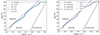 |
Fig. 4. ρc–Tc diagram for the 20 M⊙ models with different values for αov and no extra envelope mixing (log(Denv/cm2 s−1) = 0) (left panel). The right panel shows the same for αov = 0.2 and the different values for the envelope mixing, where D = log(Denv/cm2 s−1). In the left panel, the grey line shows the non-rotating model from Brinkman et al. (2021) with αov = 0.2. In the right panel, the rotating models with initial rotational velocities for 150 and 300 km/s are added as a comparison for the different treatment of envelope mixing. The blue line is the same model in both panels. The black dashed lines give a rough indication of the equations of state, that is, radiative, ideal gas, and non-relativistic electron pressure (NR electrons). The grey horizontal lines indicate a central temperature of Tc = 109. |
The change from convective carbon burning into radiative carbon burning is due to a change in the mixture of isotopes in the centre of the stars, especially in carbon and oxygen. The models that undergo radiative carbon burning have smaller C/O ratios than their convective counterparts (see column 10 of Table A.1), by almost a factor 2. This difference is due to the production channels of these isotopes. 12C and 16O are both produced during central helium burning, via two sequential reactions. The first reaction is the triple-α reaction which produces 12C. The second is a subsequent α-capture leading to the production of 16O. Once a high enough abundance of 12C is reached, the second reaction starts to dominate the energy production. For the models log(Denv/cm2 s−1) = 0, the C/O ratio decreases with the value for αov. This is due to the temperature dependence of the reactions, as the more massive cores at the end of the main sequence have higher central temperatures. The decreasing C/O ratio with increasing log(Denv/cm2 s−1) is due to a combination of the extended helium burning lifetime (see column 7 of Table A.1) and more helium being mixed into the stellar core. A lower carbon content means that less fuel is available for the carbon burning phase (12C+12C) and thus the star does not form a convective core in this phase.
The changes in composition of the stellar core at the end of helium burning due to the enhanced CBM and envelope mixing might have an indirect impact on the explodability of stars. Chieffi et al. (2021) show that a variation the carbon burning regime results in a change of the mass-radius relation (see also Sukhbold et al. 2016; Limongi & Chieffi 2020) and therefore the compactness parameter, at the time of the core collapse which can potentially impact the final fate of the star (O’Connor & Ott 2011; Ertl et al. 2016). Another potential impact of a change in the core composition is the occurrence of later stage shell mergers, such as between the carbon and oxygen burning shells (see, e.g. Ritter et al. 2018; Andrassy et al. 2020; Roberti et al. 2024), though this is beyond the scope of this work.
4. Wind yields until the end of mass loss
In this section we compare the nucleosynthetic wind yields of the various models. We compare the results with those from Brinkman et al. (2021), which are based on classical rotational mixing instead of asteroseismically calibrated internal mixing as adopted here. We start with three short-lived radioactive nuclei with half-lives less than a million years; 26Al, 36Cl, and 41Ca. Then we discuss the yields of various stable isotopes; 19F, 22Ne, and the isotopes involved in the CNO cycle, as well as the change in the surface abundance of the stable isotopes.
4.1. Short-lived radioactive nuclei
The presence of radioactive isotopes in the early Solar System is well-established as their abundances are inferred from meteoritic data showing excesses in their daughter nuclei (see for a review Lugaro et al. 2018). Here we discuss three different of such isotopes: 26Al, a short-lived radioactive isotope with a half life of 0.72 Myr (Basunia & Hurst 2016), 36Cl and 41Ca, with half lives 0.301 Myr (Nica et al. 2012) and 0.0994 Myr (Nesaraja & McCutchan 2016), respectively. These three radioactive isotopes represent the fingerprint of the local nucleosynthesis that occurred near the time and place of the birth of our Sun. Therefore, these isotopes give us clues about the environment and the circumstances of such birth (Adams 2010; Lugaro et al. 2018). In Brinkman et al. (2021) the effects of stellar rotation on the yields of single stars were investigated. For a 20 M⊙ star with αov = 0.2, the effects of stellar rotation increase the nucleosynthetic yields. Here, we compare the changes in the stellar yields due to CBM and envelope mixing as calibrated by asteroseismology of B stars.
4.1.1. Aluminium-26
26Al is a short-lived radioactive isotope which is produced during core and shell-hydrogen burning, during carbon and oxygen convective shell burning, and neon burning during the supernova explosion (see, e.g. Limongi & Chieffi 2006). In this work, we focus on the 26Al produced in hydrogen burning, which is expelled via the wind. 26Al is produced by proton captures on the stable isotope 25Mg. Its main destruction channel during hydrogen burning is the radioactive β-decay, with a small contribution from the 26Al(p,γ)27Si. During helium burning, all remaining 26Al is destroyed via the 26Al(n,α)23Na and 26Al(n,p)26Mg. 26Al is a special isotope since it has an isomeric state, with a half-life of the order of six seconds. The interaction between the ground state and the isomeric state is relatively well understood (Iliadis et al. 2010), though during hydrogen burning the temperature is such that the two states can be interpreted as separate species (see for recent overviews of 26Al Diehl et al. 2021; Laird et al. 2023).
Figure 5 shows the 26Al yields of our models. Of the models without envelope mixing, the model with the lowest value for the CBM has the highest yield, even though the mass loss is significantly smaller than for the model with the highest value, that is, 1.48 M⊙ for αov = 0.05 versus 9.55 M⊙ for αov = 0.4. This is due to the difference in the surface mass-fraction of 26Al, which is lower for the model with αov = 0.4. The longer duration of the main sequence for the models with the higher CBM, as described in Section 3, causes the difference in the yields. The difference in the duration of the main sequence, 9.49 Myr for αov = 0.4 versus 8.09 Myr for αov = 0.05, is equal to about twice the half-life of 26Al. This leads to a larger amount of 26Al to decay inside the envelope of the star before it can be expelled shortly after the main sequence. Thus, despite the larger mass loss of the models with a higher αov, this leads to a lower yield for the models with the higher CBM.
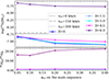 |
Fig. 5. Yields for 26Al for the different values of αov and log(Denv/cm2 s−1) (solid lines) in the upper panel. The horizontal lines indicate the yields of 20 M⊙ models with different rotational velocities (0, 150, and 300 km/s, from Brinkman et al. 2021), the dashed, dashed-dotted, and dotted lines, respectively. The lower panel shows the ratio between the yield of the reference models (log(Denv/cm2 s−1) = 0) and the models with the other values for log(Denv/cm2 s−1). |
An increase in envelope mixing has the expected effect on the yields, where more mixing leads to higher yields, especially for the highest value for the envelope mixing, as more processed material is dredged up into the outer envelope. For log(Denv/cm2 s−1) = 6.0 the yield is one order of magnitude larger than for the models without additional mixing. This effect is, to a degree, similar what happens to the yields when rotation is included (see, e.g. Sect. 4.1 of Brinkman et al. 2021) which also leads to more mixing between the core and the envelope.
In Fig. 5 we also show the yields of the 20 M⊙ models with different rotational velocities (solid, dashed-dotted, and dotted lines). The yields computed in Brinkman et al. (2021) are higher than those of the models presented in this paper, which is due to a difference in the mass-loss scheme. The models computed in Brinkman et al. (2021) lose more mass than those presented here. With less mass lost, our yields are lower for comparable models (αov = 0.2 and log(Denv/cm2 s−1) = 0). Just as increased envelope mixing by internal gravity waves increases the yields, Brinkman et al. (2021) find that increasing the rotational velocity of the stars increases the yields as well, here by a factor of 3.24.
Figure 6 shows the Kippenhahn diagrams for four of our models with the mass fraction of 26Al on the colour-scale. At the beginning of the evolution, there is no 26Al present in the stars. It is produced in the core and moved to the outer layers by the convective envelope penetrating the area vacated by the retreating hydrogen burning core (a detailed description can be found in Brinkman et al. 2019), in the case of log(Denv/cm2 s−1) = 0. With higher amounts of log(Denv/cm2 s−1), 26Al is mixed into the envelope at an earlier stage (see panel d of Figure 6). The model with αov = 0.1 and log(Denv/cm2 s−1) = 0 (panel a) has the highest mass fraction of 26Al on the surface of the star compared to the other models without envelope mixing (panels b and c) by a factor 2.7 and and 3.7, respectively. This leads to the higher yield of this model compared to the other two models with log(Denv/cm2 s−1) = 0 by a factor 1.7 and 1.5, respectively. Panel d shows the model with αov = 0.2 and log(Denv/cm2 s−1) = 6.0. The effect of the enhanced envelope mixing is visible in the early disappearance of the thermohaline mixing region (yellow shading) in the envelope, as well as in the earlier upwards diffusion of 26Al, well before the convective envelope develops, though there is still an abundance gradient. The higher amount of 26Al in the envelope combined with more mass loss leads to a strong increase in the 26Al yield (a factor of ∼21) compared to the model with αov = 0.2−log(Denv/cm2 s−1) = 0.
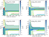 |
Fig. 6. Kippenhahn diagrams for the models with αov = 0.10, αov = 0.2, and αov = 0.4, all with log(Denv/cm2 s−1) = 0 (panels a, c, and b, respectively), as well as αov = 0.2 and log(Denv/cm2 s−1) = 6 (panel d). The solid black line is the stellar mass. The green hatched areas correspond to areas of convection, the cyan hatched areas to CBM, the red hatched areas to semi-convection, and the yellow hatched areas to thermohaline mixing. The blue dotted line indicates the hydrogen-depleted core. The red and green dotted lines indicate the helium- and carbon-depleted cores, respectively. The colour scale shows the 26Al mass fraction as a function of the mass coordinate and time. |
4.1.2. 36Cl and 41Ca
36Cl and 41Ca are short-lived radioactive isotopes which are produced during core helium burning and during the explosive burning in a supernova (see, e.g. Pignatari et al. 2016; Limongi & Chieffi 2018). Both isotopes are mainly produced by neutron captures on the stable isotopes 35Cl and 40Ca, respectively. The neutrons needed for this process are produced by the 22Ne(α,n)25Mg reaction (see, e.g. Arnould et al. 1997), though in the earliest stages 13C(α,n)16O has a minor contribution. For both isotopes, the main destruction channel is through further neutron captures, either (n,α) or (n,γ).
Figure 7 shows the 36Cl (left panel) and 41Ca (right panel) wind yields of the model. For the models with log(Denv/cm2 s−1) = 0−4.5, the yields are very low, all of the order of 10−19 (10−20) M⊙ for 36Cl (41Ca). This is because 36Cl and 41Ca are produced deep inside the stellar interior and need to be brought up to the surface to significantly contribute to the yields. The surface enrichment can be achieved in two manners, (i) by stripping enough mass off the star via the stellar wind to expose the inner parts of the star and (ii) by diffusing the material produced in the stellar core up to the surface. For the models with log(Denv/cm2 s−1) = 0−4.5, independent of the CBM, the mass loss until the onset of helium burning is not enough to expose the innermost layers of the star, nor is the timescale of helium burning long enough to get any significant diffusion of 36Cl (41Ca) to the stellar surface. For the models with log(Denv/cm2 s−1) = 6.0, the mass loss is also not strong enough to expose the inner layers. However, in this case, the helium burning timescale is long enough for material to be diffused into the envelope, where the convective outer layer brings the material to the surface. This leads to strongly enhanced yields, with a factor 4.18 × 10¹¹ (7.35 × 10¹¹) to 3.08 × 10¹⁰ (1.10 × 10¹¹) from αov = 0.05 to αov = 0.4. This is visible when comparing the panels of Fig. 8. It shows the Kippenhahn diagrams for the models with αov = 0.2 and log(Denv/cm2 s−1) = 0 (panel a) and log(Denv/cm2 s−1) = 6.0 (panel b). The colour-scale shows the 41Ca-mass fraction inside the stars. The distribution of 36Cl looks similar. For both the model with log(Denv/cm2 s−1) = 0 and log(Denv/cm2 s−1) = 6, the envelope becomes convective after hydrogen burning and material deeper in the star can be brought to the surface. However, for log(Denv/cm2 s−1) = 0, this does not happen, while for log(Denv/cm2 s−1) = 6.0, the surface becomes enriched in 41Ca (36Cl). This is due to the still-present envelope mixing.
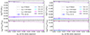 |
Fig. 7. Same as Fig. 5, but for 36Cl (left) and 41Ca (right). The lower panels show the ratio between the yield of the reference models (log(Denv/cm2 s−1) = 0) and the models with the other values for log(Denv/cm2 s−1). Mind that unlike in Fig. 5, here the y-scale for the ratio is in log. |
When comparing the wind yields for all models with log(Denv/cm2 s−1) = 6.0, they decrease slightly with increasing αov. This is due to a combination of the duration of the helium burning phase and the mass loss beyond helium burning. The helium burning phase is shorter for the higher values for the CBM, 1.15 Myr for αov = 0.05 versus 0.66 Myr for αov = 0.4, which means that less 41Ca (or 36Cl) can reach the surface. Also, the model with αov = 0.05 loses 0.19 M⊙ after helium burning is finished, while the model with αov = 0.4 loses only 0.1 M⊙. This combination leads to a wind yield of a factor 8.0 (3.9) higher for αov = 0.05 for 36Cl (41Ca).
An interesting feature in Fig. 8b is that 41Ca is visibly mixed out of the core, but only a part reaches the surface of the star. Instead, a band with a higher abundance is formed, roughly at 7.0 M⊙. Even though the mixing is relatively strong, the helium burning timescale is not long enough to diffuse the produced 41Ca towards the surface and into the convective layer. This leads to a build-up of 41Ca above the convective helium-burning core, but below the border of the envelope and the hydrogen-depleted core.
Compared to the yields presented here, the 36Cl and 41Ca yields from Brinkman et al. (2021) are lower, even for the models that include rotational mixing. This is because the rotational velocity of the envelope has gone down and along with it the efficiency of the mixing in the envelope, while in the asteroseismic models the envelope mixing is still at full strength. Therefore, the surface abundance is lower for the models from Brinkman et al. (2021), leading to lower wind yields.
4.2. Stable nuclei
4.2.1. 19F and 22Ne
Both 19F and 22Ne are stable isotopes which are present in the stars from birth and their initial abundances therefore scale with the initial metallicity of the star. Figure 9 shows the yields for 19F (left panel) and 22Ne (right panel). The initial mass of the isotopes present in the stars is given by the red horizontal lines. None of the models presented here have a net positive yield for 19F and only one model has a positive yield for 22Ne.
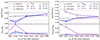 |
Fig. 9. Same as Fig. 5, but for 19F (left) and 22Ne (right). The lower panels show the ratio between the yield of the reference models (log(Denv/cm2 s−1) = 0) and the models with the other values for log(Denv/cm2 s−1). |
4.3. Fluorine-19
19F is of interest because its galactic source is still uncertain. Meynet & Arnould (2000) have shown that Wolf-Rayet stars (generally Mi≥ 30 M⊙ at solar metallicity) can contribute significantly to the galactic 19F abundance while Palacios et al. (2005) found that the same stars are unlikely to be the source of galactic 19F, when including updated mass-loss prescriptions and reaction rates. The discussion around 19F was rekindled by Jönsson et al. (2014a,b, 2017) and Abia et al. (2019), who re-analysed observations of 19F and proposed that asymptotic giant branch stars are the most likely source of cosmic 19F. Other works suggest that 19F may come from rotating massive stars at very low metallicity (see, e.g. Prantzos et al. 2018; Grisoni et al. 2020; Franco et al. 2021; Roberti et al. 2024). Though, due to the remaining uncertainty in both the mass-loss prescriptions and the reaction rates (see e.g. Stancliffe et al. 2005; Ugalde et al. 2008), Wolf-Rayet stars in general cannot be excluded as the sources of galactic 19F (for a recent overview, see e.g. Ryde et al. 2020). On the other hand, Womack et al. (2023) concluded that Wolf-Rayet stars are not an important contributor. Even though the mass of the models presented here is lower than the Wolf-Rayet limit, the enhanced envelope mixing might have been expected to have an effect.
19F is typically destroyed in the hydrogen burning core due to proton-captures, via the 19F(p, α)16O reaction, which is part of the CNO cycles. It is produced during helium burning by a reaction chain starting at 14N; 14N(α,γ)18F(,e+)18O(p,α)15N(α,γ)19F, as first introduced by Forestini et al. (1992). It is then rapidly destroyed afterwards due to α-captures (Meynet & Arnould 2000). This is well visible in Fig. 10, where the colour-scale indicates the mass-fraction of 19F present in the star. At birth, there is some 19F present in the star, which is clearly visible in the envelope. In the hydrogen burning core, 19F is rapidly destroyed. In the left panel (log(Denv/cm2 s−1) = 0), there is no 19F present below the outermost mass-coordinate of the hydrogen-burning core (10 M⊙), while for the right panel (log(Denv/cm2 s−1) = 6), the envelope mixing keeps the mass fraction smoothed out in the envelope. During helium burning, which starts at log(time until collapse/yrs) = 6.0 in Fig. 10, 19F is produced in the stellar core. In the left panel (αov = 0.2 and log(Denv/cm2 s−1) = 0), all the 19F remains in the core. For the right panel (αov = 0.2 and log(Denv/cm2 s−1) = 6), 19F is mixed out, as can be seen by the darker shading above the convective helium burning core. Towards the end of helium burning, the central abundance is significantly less and also in the envelope it is reduced, until the helium burning shell becomes active around log(time until collapse/yrs) = 4.0. Panel b of Fig. 10 shows clearly that, despite the enhanced envelope mixing, the 19F produced in the core is not reaching the surface, which has a comparable mass-fraction over the entire evolution. The 19F produced in the core is mixed out to roughly the top of the hydrogen-depleted core (blue dotted line in Fig. 10). The overall effect is that these models have negative 19F net yields over the whole range (see left panel of Fig. 9), as there is more destruction in the star than 19F leaving the star in the stellar winds.
The red line at the top of the left panel of Fig. 9 is the initial amount of 19F present in the star. None of the models have positive net yields. Compared to the model with log(Denv/cm2 s−1) = 0, all models with log(Denv/cm2 s−1) = 6 have larger yields, except for αov = 0.4, where the yield is lower. This is because, despite having the largest amount of mass loss, this model also has the longest main sequence lifetime. The strong interaction between the stellar core and stellar envelope leads to an increased destruction of 19F, which lowers the yield. Also, the shorter duration of helium burning reduces the amount of 19F mixed into the envelope during helium burning, which together leads to a lower wind yield for this model than for the model without enhanced envelope mixing. The difference in mass lost during helium burning causes the differences in the yields aside from the enhanced destruction. Overall, the yields are fairly comparable, which is mainly because the 19F expelled was already present in the star from birth and is not newly synthesised.
When comparing the yields to those in Brinkman et al. (2021), we find comparable results for rotational velocities of 0 and 150 km/s, for the lowest envelope mixing. The model with the largest rotational velocity has a lower yield by a factor of ∼2, which is due to the destruction of 19F, enhanced by the induced rotational mixing.
4.4. Neon-22
22Ne is interesting to study because it is the main neutron sources for the slow neutron-capture process (s-process), via the 22Ne(α,n)25Mg reaction in massive stars. The amount of 22Ne and its distribution throughout the star affects the amount of s-process isotopes produced. Because we consider a star of 20 M⊙, this is mainly the weak s-process, which produces the s-process isotopes between iron and strontium, though also slightly beyond that, such as 107Pd (Pignatari et al. 2010). The extra mixing could potentially produce more 22Ne, which could lead to a boost in the s-process creating the isotopes beyond the first peak as shown by for example Pignatari et al. (2008), Frischknecht et al. (2012), Choplin et al. (2018), Limongi & Chieffi (2018). However, these studies mainly consider low metallicity stars, while we consider solar metallicity.
In the right panel of Fig. 9, the yields for 22Ne are shown. For the models with log(Denv/cm2 s−1) = 0−4.5, they follow a similar trend as for 19F. The 22Ne wind yields increase strongly for αov = 0.05, with almost a factor 6, while for αov = 0.4, the wind yields barely increase compared to the other models with the same value for the CBM. This is due to a combination of when 22Ne is produced the difference in the duration of the hydrogen and helium burning phases between the different models and a difference in the mass loss history.
Figure 11 shows the 22Ne-content for the models with αov = 0.2 and log(Denv/cm2 s−1) = 0 (left) and log(Denv/cm2 s−1) = 6 (right). 22Ne is partially destroyed during hydrogen-burning in the core by proton-captures via 22Ne(p,γ)23Na, which is part of the Ne-Na-cycle. Beyond hydrogen burning, 22Ne is produced again during helium burning, first in the core and then in the helium burning shell by a chain of α-captures on the 14N left by the CNO cycle. Part of the 22Ne produced here is then destroyed by α-captures.
The strong increase in the wind yield from log(Denv/cm2 s−1) = 0 and log(Denv/cm2 s−1) = 6 for αov = 0.05 is due to the large difference in the mass loss between the two models, 5.2 M⊙ versus 9.1 M⊙. This is similar for αov = 0.1 and αov = 0.2, though the difference decreases with increasing CBM. For αov = 0.4, the 22Ne yields are all comparable, which has to do with competing mechanisms. While the mass loss for the model with log(Denv/cm2 s−1) = 6 is the largest with 10.17 M⊙, the combination of the longest hydrogen burning lifetime with the shortest helium burning lifetime leads to a comparable yield as αov = 0.4 and log(Denv/cm2 s−1) = 0. When the hydrogen burning lifetime increases with more envelope mixing, 22Ne is mixed from the envelope into the core, where it is destroyed. This reduces the amount of 22Ne in the envelope and brings the yield down. Also, due to the shorter helium burning lifetime, the 22Ne produced in the stellar core has limited time to diffuse into the envelope to contribute to the stellar yield. All together, this leads to the models with αov = 0.4 having comparable yields.
For the models of Brinkman et al. (2021), the yields decrease with increasing rotational velocity. This is due to the enhanced mixing between the stellar envelope and the stellar core, just as described above. For the model with an initial rotational velocity of 300 km/s the interaction is the strongest, leading to the lowest yield.
4.4.1. The stable isotopes of the CNO cycle
The isotopes of the CNO cycle are interesting because they are among the most abundant elements in the Universe. The origin of the CNO ratios as measured in stardust grains has been extensively studied (see, e.g. Romano & Matteucci 2003; Romano et al. 2019; Kobayashi et al. 2020, and references therein). However, their astrophysical sources, especially for carbon, are not well understood (see, e.g. Kobayashi et al. 2020). At the same time, due to their large abundance, these elements can be measured in the atmospheres of stars. Especially 14N has been used as a measure of the rotational mixing (see, e.g. Maeder & Meynet 2000). Here we consider the yields of the most abundant isotopes of the CNO cycle and briefly discuss how the surface ratios of these isotopes change over the evolution of the star. The solar ratios of the CNO isotopes are well-known from meteoretic data. While the short-lived radioactive isotopes are produced close in time and location to the early Solar System, the CNO isotopes have a slow build-up over the galactic history. Therefore, any potential source of the short-lived radioactive isotopes must have a comparable mixture of CNO isotopes to the early Solar System, or such that the ratios do not change beyond their error-bars (Gounelle & Meibom 2007).
Figure 12 shows the yields of seven isotopes, 12, 13C, 14, 15N, and 16 − 18O (the last two isotopes are combined in one panel). In all panels, the initial amount of the isotope present in the models is given by the red line. Overall, the isotopes can be split into three categories, (i) those that are produced and destroyed during helium burning, 12C and 18O, (ii) those that are abundantly present at the end of hydrogen burning and are destroyed during helium burning, 13C and 14N, and (iii) those that are produced during helium burning and survive the burning stage, 15N, 16O, and 17O. The first group shows a comparable behaviour to 19F, the second and third group show a comparable behaviour to 22Ne. All isotopes are initially turned into 14N as part of the CNO cycles during core hydrogen burning and then reach an equilibrium value. Nearly all net yields of the isotopes of the CNO cycle are negative, except for 13C and 14N.
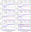 |
Fig. 12. Yields for the main isotopes of the CNO cycle for the different values of αov and log(Denv/cm2 s−1) (dots connected by lines). The horizontal lines indicate the yields of 20 M⊙ models (dashed, dashed-dotted, and dotted lines) with different rotational velocities (0, 150, and 300 km/s, from Brinkman (2022)). The isotopes are 12C, 13C, 14N, 15N, 16O, and in the last panel 17O (solid lines) and 18O (dash-dotted lines). In this panel, the grey horizontal lines are for 17O and the black horizontal lines are for 18O. The lower panels show the ratio between the yield of the reference models (log(Denv/cm2 s−1) = 0) and the models with the other values for log(Denv/cm2 s−1). |
The CNO cycle is a catalytic cycle, meaning that as soon as an equilibrium is reached, none of the isotopes involved are overall created or destroyed. The slowest reaction of the CNO cycle is the 14N(p,γ)15O, leading to a build-up of 14N during hydrogen burning. Figure 13 shows how the 12C/14N surface ratio starts to change at the terminal-age main sequence (TAMS), mainly for log(Denv/cm2 s−1) = 6.0 (purple symbols). At the onset of helium burning deeper layers of the star, where the composition is changed due to the earlier burning, are exposed due to mass loss and the ratios have strongly changed compared to the zero-age main sequence. For the 14N/16O ratio the changes are less visible at the TAMS and mainly occur at the onset of helium burning. This means that, despite the enhanced mixing in the envelope, the surface of the star is not strongly enriched in processed CNO material during the main sequence.
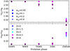 |
Fig. 13. Change of the C/N and N/O ratios on the surface of the models given at seven different times in the evolution; at the zero-age main sequence (ZAMS), half-way the main sequence (MMS), at the terminal-age main sequence (TAMS), on the Hertzsprung gap (HRG), and at the onset of helium burning (ZAHeB). The symbols are for the different values for αov while the colours indicate the different amounts of log(Denv/cm2 s−1) in the same way as in the previous figures. |
4.5. Nitrogen
Figure 14 shows the internal abundance profiles of 14N at four moments in the stellar evolution. Our models (blue and purple lines) are compared with the non-rotating and fastest rotating models from Brinkman et al. (2021) (grey lines). Halfway up the main sequence (top left panel) and at the TAMS (top right panel), the model with the highest rotational velocity (dotted line, 300 km/s) has an enhanced surface abundance of 14N, while the other models do not. It shows that the enhanced envelope mixing smooths out the nitrogen build-up on top of the hydrogen burning core (area up to ∼10 M⊙). The non-rotating model has slightly higher 14N values just outside of the hydrogen-burning core due the larger value of f0, which leads to more mixing from below the convective boundary. On the Hertzsprung-gap (bottom left panel), the semi-convective mixing in the model with log(Denv/cm2 s−1) = 0 causes the step profile while the model with log(Denv/cm2 s−1) = 6.0 has a smooth internal distribution of 14N. At the onset of helium burning, 14N is destroyed in the core (below ∼5 M⊙). Just outside the helium burning core there is a build-up of 14N. In the envelope the levels of 14N are increased due to the hydrogen burning shell, leading to the highest surface mass-fraction for the rotating model.
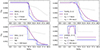 |
Fig. 14. 14N abundance profiles at four different phases of the evolution of the models with αov = 0.2 and log(Denv/cm2 s−1) = 0 (blue) and 6 (purple). The top left panel shows the profiles halfway the main sequence (MMS), the top right at the end of the main sequence (TAMS), the bottom left at the beginning of the Hertzsprung gap (HRG), and the bottom right at the onset of helium burning (ZAHeB). The grey lines a (dashed for 0 km/s and dotted for 300 km/s) are from Brinkman (2022). |
The yields for 14N and 15N are given in the central panels of Fig. 12. The yields for 14N follow the same trend as 22Ne. All yields with αov = 0.2 and 0.4 as well as the models with log(Denv/cm2 s−1) = 6.0 give positive net yields. For the other models the yields are close to the initial amount of 14N present in the star.
4.6. Carbon
The yields for 12C and 13C are given in the top panels of Fig. 12. During helium burning, 12C is produced by the triple-α process. Some of this 12C is then turned into 16O via subsequent α-capture. Due to the combination of production and destruction, the yields of 12C show a similar behaviour as for 19F. None of the models presented here have a positive net yield for 12C. For the models of Brinkman (2022), the 12C yields decrease with increasing initial rotational velocity. As for the previous isotopes, this is due to the enhanced mixing between the core and the envelope. Like for 19F, the models with log(Denv/cm2 s−1) = 6.0 have increased yields compared to the model without envelope mixing instead of decreasing yields, though at most the yields increase by a factor 1.9.
13C is completely destroyed by α-captures via the 13C(α,n)16O reaction. This produces the first neutron burst for the production of 36Cl and 41Ca at the beginning of helium burning. The 13C that is expelled via the stellar wind into the interstellar medium, however, is produced during hydrogen-burning as part of the CNO cycle. It therefore has a similar behaviour as 14N. 13C(p,γ)14N is the second-slowest reaction of the CNO cycle, making 13C the second most abundant isotope of the cycle. 13C is produced when the initially more abundant 12C is converted into 13N, which then decays into 13C. Like for 14N, 13C is mixed into the envelope, leading to a positive net yield for the models with a strong enough interaction between the core and the envelope (αov = 0.2 and 0.4, and all models with log(Denv/cm2 s−1) = 6.0).
The 13C yields from Brinkman (2022) increase for an initial rotational velocity of 150 km/s, but then decrease for an initial rotational velocity of 300 km/s. This is because the previously mentioned catalytic nature of the CNO cycle. The more 14N is removed from the core, the more 13C is converted into 14N, but the compensation is reduced due to the removal of 14N. This then reduces the yields. In comparison, the models with log(Denv/cm2 s−1) = 6.0 behave more like those with an initial rotational velocity of 150 km/s.
4.7. Oxygen
The lower panels of Fig. 12 give the yields of 16 − 18O. 16O behaves comparable to 22Ne. However, the initial abundance of 16O is very high and due to its late production during helium burning, all the net yields are negative. For 17O and 18O, none of the net yields are positive either. 17O behaves comparable to 22Ne due to its production in the late stages of core helium burning. All the net yields are negative for this isotope. 18O is produced as part of the following reaction chain from 14N into 22Ne; 14N(α,γ)18F(e+)18O(α,γ)22Ne. In the final step, by the end of helium burning, it is almost completely destroyed again. This leads to negative net yields over the whole range of models following the trend of 19F.
5. Conclusions
In this first study of the effect of enhanced CBM and enhanced envelope mixing based on a mixing profile from internal gravity waves, with their strengths based on asteroseismic calibrations, we reach the following conclusions:
-
On the main sequence, the effects on the stellar evolution are comparable to other studies considering CBM (e.g. Kaiser et al. 2020), or the effects of rotationally induced mixing (see, e.g. Ekström et al. 2012; Limongi & Chieffi 2018; Brinkman et al. 2021, and many others).
-
During helium burning, enhanced envelope mixing leads to longer helium burning timescales and smaller helium-depleted cores at the end of helium burning. This suggests that while CBM is the dominant source of mixing on the main sequence, where the envelope mixing only has a strong impact for log(Denv/cm2 s−1) = 6, the envelope mixing is the more important mechanism during core helium burning.
-
The combination of enhanced envelope and CBM has a strong impact on the carbon-to-oxygen ratio at the end of helium burning. This leads an earlier transition from convective to radiative carbon burning than is seen in the literature. This can potentially have strong effects on the final fate of massive stars and on the explosive nucleosynthesis, as changes in this ratio change the mass-radius relation (compactness) and the potential occurrence of shell mergers.
-
From log(Denv/cm2 s−1) = 0 to log(Denv/cm2 s−1) = 4.5, the nucleosynthetic yields do not significantly increase. This is because the envelope mixing is a diffusive process and the timescale is too short for significant mixing up to the surface to take place. The main increase happens only for log(Denv/cm2 s−1) = 6, for which the diffusive mixing is strong enough for the isotopes to reach the upper layers of the envelope on the evolutionary timescales of the models. Especially for 36Cl and 41Ca the increase is significant with ∼11 orders of magnitude compared to the models without enhanced envelope mixing.
-
For 26Al an increase in the convective boundary leads to lower yields because the longer main sequence lifetimes imply an increased decay of the isotope inside the star.
-
Out of the stables isotopes, only 13C and 14N have mainly positive net yields and even for those not over the full range of models. For most of the stable isotopes the net yields are negative, as is expected for this mass.
We also find that the surface abundance ratios of our models do not significantly change during the main sequence (see Fig. 13), except for the models with the largest amount of envelope mixing (log(Denv/cm2 s−1) = 6). At the start of helium burning (ZAHeB), all stars show an enhancement of 14N on the surface, which is not due to envelope mixing, but due to the stellar winds exposing the processed layers of the stellar interior. Our models do not favour a strong nitrogen enrichment of the surface on the main sequence, even for log(Denv/cm2 s−1) = 6 the enrichment is moderate compared to the rotating model from Brinkman (2022) (dotted grey line in Fig. 14), which is in line with Aerts et al. (2014). In future work we will study the interplay between rotational and internal gravity wave mixing to compute surface abundances and nucleosynthetic yields.
Further future work includes, but is not limited to, the following:
-
Consideration of different shapes of the mixing profile for the envelopes, based on Ω(r) and dΩ(r)dr profiles, see Mombarg et al. (2022).
-
Consideration of time-dependent CBM and time-dependent envelope mixing, see Varghese et al. (2023).
-
Inclusion of joint rotational and internal gravity wave mixing.
-
Extension of the current set of models to lower and higher masses to allow for comparison with observations of detached binary systems and comparison with samples of observed stars.
-
Extension of the models to cover the final phases of the stellar evolution up to core collapse, which can then be used for nucleosynthetic post-processing of the pre-supernova phase to determine the weak s-process yields, as well as the possibility to explode the models and study the impact of envelope mixing based on internal gravity waves on the supernova yields.
Acknowledgments
HEB thanks the MESA team for making their code publicly available, Ebraheem Farag and Jared Goldberg for their advice on stellar modelling, as well as Rob Farmer for debugging the part of the code related to the reaction rates, and Matthias Fabry for general help with debugging. The research leading to these results has received funding from the KU Leuven Research Council (grant C16/18/005: PARADISE), from the Research Foundation Flanders (FWO) under grant agreement G089422N, as well as from the BELgian federal Science Policy Office (BELSPO) through PRODEX grant PLATO. MM acknowledges support from the Research Foundation Flanders (FWO) by means of a PhD scholarship under project No. 11F7120N.
References
- Abia, C., Cristallo, S., Cunha, K., de Laverny, P., & Smith, V. V. 2019, A&A, 625, A40 [CrossRef] [EDP Sciences] [Google Scholar]
- Adams, F. C. 2010, ARA&A, 48, 47 [NASA ADS] [CrossRef] [Google Scholar]
- Aerts, C. 2021, Rev. Mod. Phys., 93, 015001 [Google Scholar]
- Aerts, C., Thoul, A., Daszyńska, J., et al. 2003, Science, 300, 1926 [Google Scholar]
- Aerts, C., Molenberghs, G., Kenward, M. G., & Neiner, C. 2014, ApJ, 781, 88 [Google Scholar]
- Aerts, C., Mathis, S., & Rogers, T. M. 2019, ARA&A, 57, 35 [Google Scholar]
- Andrassy, R., Herwig, F., Woodward, P., & Ritter, C. 2020, MNRAS, 491, 972 [NASA ADS] [CrossRef] [Google Scholar]
- Angelou, G. C., Bellinger, E. P., Hekker, S., et al. 2020, MNRAS, 493, 4987 [NASA ADS] [CrossRef] [Google Scholar]
- Angulo, C., Arnould, M., Rayet, M., et al. 1999, Nucl. Phys. A, 656, 3 [Google Scholar]
- Arnould, M., Paulus, G., & Meynet, G. 1997, A&A, 321, 452 [NASA ADS] [Google Scholar]
- Aver, E., Olive, K. A., Porter, R. L., & Skillman, E. D. 2013, JCAP, 2013, 017 [Google Scholar]
- Banerjee, P., Heger, A., & Qian, Y.-Z. 2019, ApJ, 887, 187 [Google Scholar]
- Basunia, M., & Hurst, A. 2016, Nucl. Data Sheets, 134, 75 [NASA ADS] [CrossRef] [Google Scholar]
- Björklund, R., Sundqvist, J. O., Puls, J., & Najarro, F. 2021, A&A, 648, A36 [EDP Sciences] [Google Scholar]
- Böhm-Vitense, E. 1958, Z. Astrophys., 46, 108 [Google Scholar]
- Brinkman, H. E. 2022, Ph.D. Thesis, University of Szeged, Hungary [Google Scholar]
- Brinkman, H. E., Doherty, C. L., Pols, O. R., et al. 2019, ApJ, 884, 38 [NASA ADS] [CrossRef] [Google Scholar]
- Brinkman, H. E., den Hartog, H., Doherty, C. L., Pignatari, M., & Lugaro, M. 2021, ApJ, 923, 47 [NASA ADS] [CrossRef] [Google Scholar]
- Briquet, M., Morel, T., Thoul, A., et al. 2007, MNRAS, 381, 1482 [Google Scholar]
- Briquet, M., Neiner, C., Aerts, C., et al. 2012, MNRAS, 427, 483 [NASA ADS] [CrossRef] [Google Scholar]
- Burssens, S., Bowman, D. M., Michielsen, M., et al. 2023, Nat. Astron., 7, 913 [NASA ADS] [CrossRef] [Google Scholar]
- Charpinet, S., Van Grootel, V., Randall, S. K., et al. 2010, Highlights Astron., 15, 357 [Google Scholar]
- Charpinet, S., Van Grootel, V., Fontaine, G., et al. 2011, A&A, 530, A3 [NASA ADS] [CrossRef] [EDP Sciences] [Google Scholar]
- Chieffi, A., & Limongi, M. 2013, ApJ, 764, 21 [Google Scholar]
- Chieffi, A., Roberti, L., Limongi, M., et al. 2021, ApJ, 916, 79 [NASA ADS] [CrossRef] [Google Scholar]
- Choplin, A., Hirschi, R., Meynet, G., et al. 2018, A&A, 618, A133 [NASA ADS] [CrossRef] [EDP Sciences] [Google Scholar]
- Claret, A., & Torres, G. 2017, ApJ, 849, 18 [Google Scholar]
- Cyburt, R. H., Amthor, A. M., Ferguson, R., et al. 2010, ApJS, 189, 240 [NASA ADS] [CrossRef] [Google Scholar]
- Deheuvels, S., Brandão, I., Silva Aguirre, V., et al. 2016, A&A, 589, A93 [NASA ADS] [CrossRef] [EDP Sciences] [Google Scholar]
- Diehl, R., Lugaro, M., Heger, A., et al. 2021, PASA, 38, e062 [NASA ADS] [CrossRef] [Google Scholar]
- Dupret, M. A., Thoul, A., Scuflaire, R., et al. 2004, A&A, 415, 251 [NASA ADS] [CrossRef] [EDP Sciences] [Google Scholar]
- Ekström, S., Meynet, G., Maeder, A., & Barblan, F. 2008, A&A, 478, 467 [Google Scholar]
- Ekström, S., Georgy, C., Eggenberger, P., et al. 2012, A&A, 537, A146 [Google Scholar]
- Ertl, T., Janka, H. T., Woosley, S. E., Sukhbold, T., & Ugliano, M. 2016, ApJ, 818, 124 [NASA ADS] [CrossRef] [Google Scholar]
- Farmer, R., Fields, C. E., Petermann, I., et al. 2016, ApJS, 227, 22 [NASA ADS] [CrossRef] [Google Scholar]
- Forestini, M., Goriely, S., Jorissen, A., & Arnould, M. 1992, A&A, 261, 157 [NASA ADS] [Google Scholar]
- Franco, M., Coppin, K. E. K., Geach, J. E., et al. 2021, Nat. Astron., 5, 1240 [Google Scholar]
- Frischknecht, U., Hirschi, R., & Thielemann, F. K. 2012, A&A, 538, L2 [NASA ADS] [CrossRef] [EDP Sciences] [Google Scholar]
- Georgy, C., Ekström, S., Granada, A., et al. 2013, A&A, 553, A24 [NASA ADS] [CrossRef] [EDP Sciences] [Google Scholar]
- Ghasemi, H., Moravveji, E., Aerts, C., Safari, H., & Vučković, M. 2017, MNRAS, 465, 1518 [Google Scholar]
- Gounelle, M., & Meibom, A. 2007, ApJ, 664, L123 [CrossRef] [Google Scholar]
- Grisoni, V., Romano, D., Spitoni, E., et al. 2020, MNRAS, 498, 1252 [NASA ADS] [CrossRef] [Google Scholar]
- Guenther, D. B., Demarque, P., & Gruberbauer, M. 2014, ApJ, 787, 164 [NASA ADS] [CrossRef] [Google Scholar]
- Heger, A., Langer, N., & Woosley, S. E. 2000, ApJ, 528, 368 [NASA ADS] [CrossRef] [Google Scholar]
- Herwig, F. 2000, A&A, 360, 952 [NASA ADS] [Google Scholar]
- Herwig, F., Bloecker, T., Schoenberner, D., & El Eid, M. 1997, A&A, 324, L81 [NASA ADS] [Google Scholar]
- Hirschi, R., Meynet, G., & Maeder, A. 2004, A&A, 425, 649 [NASA ADS] [CrossRef] [EDP Sciences] [Google Scholar]
- Hirschi, R., Meynet, G., & Maeder, A. 2005, A&A, 433, 1013 [NASA ADS] [CrossRef] [EDP Sciences] [Google Scholar]
- Iliadis, C., Longland, R., Champagne, A. E., & Coc, A. 2010, Nucl. Phys. A, 841, 323 [NASA ADS] [CrossRef] [Google Scholar]
- Imbriani, G., Costantini, H., Formicola, A., et al. 2005, Eur. Phys. J. A, 25, 455 [Google Scholar]
- Jermyn, A. S., Bauer, E. B., Schwab, J., et al. 2023, ApJS, 265, 15 [NASA ADS] [CrossRef] [Google Scholar]
- Johnston, C. 2021, A&A, 655, A29 [NASA ADS] [CrossRef] [EDP Sciences] [Google Scholar]
- Jönsson, H., Ryde, N., Harper, G. M., Richter, M. J., & Hinkle, K. H. 2014a, ApJ, 789, L41 [CrossRef] [Google Scholar]
- Jönsson, H., Ryde, N., Harper, G. M., et al. 2014b, A&A, 564, A122 [NASA ADS] [CrossRef] [EDP Sciences] [Google Scholar]
- Jönsson, H., Ryde, N., Spitoni, E., et al. 2017, ApJ, 835, 50 [CrossRef] [Google Scholar]
- Kaiser, E. A., Hirschi, R., Arnett, W. D., et al. 2020, MNRAS, 496, 1967 [Google Scholar]
- Kobayashi, C., Karakas, A. I., & Lugaro, M. 2020, ApJ, 900, 179 [Google Scholar]
- Kudritzki, R.-P., & Puls, J. 2000, ARA&A, 38, 613 [Google Scholar]
- Laird, A. M., Lugaro, M., Kankainen, A., et al. 2023, J. Phys. G Nucl. Phys., 50, 033002 [CrossRef] [Google Scholar]
- Langer, N. 2012, ARA&A, 50, 107 [CrossRef] [Google Scholar]
- Limongi, M., & Chieffi, A. 2006, ApJ, 647, 483 [NASA ADS] [CrossRef] [Google Scholar]
- Limongi, M., & Chieffi, A. 2018, ApJS, 237, 13 [NASA ADS] [CrossRef] [Google Scholar]
- Limongi, M., & Chieffi, A. 2020, ApJ, 902, 95 [NASA ADS] [CrossRef] [Google Scholar]
- Lugaro, M., Ott, U., & Kereszturi, Á. 2018, Progr. Part. Nucl. Phys., 102, 1 [NASA ADS] [Google Scholar]
- Maeder, A., & Meynet, G. 2000, ARA&A, 38, 143 [Google Scholar]
- Mathis, S., Palacios, A., & Zahn, J. P. 2004, A&A, 425, 243 [NASA ADS] [CrossRef] [EDP Sciences] [Google Scholar]
- Meynet, G., & Arnould, M. 2000, A&A, 355, 176 [NASA ADS] [Google Scholar]
- Michielsen, M., Pedersen, M. G., Augustson, K. C., Mathis, S., & Aerts, C. 2019, A&A, 628, A76 [NASA ADS] [CrossRef] [EDP Sciences] [Google Scholar]
- Michielsen, M., Aerts, C., & Bowman, D. M. 2021, A&A, 650, A175 [NASA ADS] [CrossRef] [EDP Sciences] [Google Scholar]
- Mombarg, J. S. G., Van Reeth, T., Pedersen, M. G., et al. 2019, MNRAS, 485, 3248 [NASA ADS] [CrossRef] [Google Scholar]
- Mombarg, J. S. G., Dotter, A., Rieutord, M., et al. 2022, ApJ, 925, 154 [NASA ADS] [CrossRef] [Google Scholar]
- Montalbán, J., Miglio, A., Noels, A., et al. 2013, ApJ, 766, 118 [Google Scholar]
- Moravveji, E., Aerts, C., Pápics, P. I., Triana, S. A., & Vandoren, B. 2015, A&A, 580, A27 [NASA ADS] [CrossRef] [EDP Sciences] [Google Scholar]
- Moravveji, E., Townsend, R. H. D., Aerts, C., & Mathis, S. 2016, ApJ, 823, 130 [NASA ADS] [CrossRef] [Google Scholar]
- Nesaraja, C., & McCutchan, E. 2016, Nucl. Data Sheets, 133, 120 [NASA ADS] [CrossRef] [Google Scholar]
- Nica, N., Cameron, J., & Singh, J. 2012, Nucl. Data Sheets, 113, 25 [NASA ADS] [Google Scholar]
- Nieuwenhuijzen, H., & de Jager, C. 1990, A&A, 231, 134 [NASA ADS] [Google Scholar]
- Noll, A., Deheuvels, S., & Ballot, J. 2021, A&A, 647, A187 [EDP Sciences] [Google Scholar]
- Nomoto, K., Kobayashi, C., & Tominaga, N. 2013, ARA&A, 51, 457 [CrossRef] [Google Scholar]
- Nugis, T., & Lamers, H. J. G. L. M. 2000, A&A, 360, 227 [NASA ADS] [Google Scholar]
- O’Connor, E., & Ott, C. D. 2011, ApJ, 730, 70 [Google Scholar]
- Palacios, A., Arnould, M., & Meynet, G. 2005, A&A, 443, 243 [NASA ADS] [CrossRef] [EDP Sciences] [Google Scholar]
- Paxton, B., Bildsten, L., Dotter, A., et al. 2011, ApJS, 192, 3 [Google Scholar]
- Paxton, B., Cantiello, M., Arras, P., et al. 2013, ApJS, 208, 4 [Google Scholar]
- Paxton, B., Marchant, P., Schwab, J., et al. 2015, ApJS, 220, 15 [Google Scholar]
- Paxton, B., Schwab, J., Bauer, E. B., et al. 2018, ApJS, 234, 34 [NASA ADS] [CrossRef] [Google Scholar]
- Paxton, B., Smolec, R., Schwab, J., et al. 2019, ApJS, 243, 10 [Google Scholar]
- Pedersen, M. G. 2022, ApJ, 930, 94 [NASA ADS] [CrossRef] [Google Scholar]
- Pedersen, M. G., Aerts, C., Pápics, P. I., et al. 2021, Nat. Astron., 5, 715 [NASA ADS] [CrossRef] [Google Scholar]
- Pignatari, M., Gallino, R., Meynet, G., et al. 2008, ApJ, 687, L95 [Google Scholar]
- Pignatari, M., Gallino, R., Heil, M., et al. 2010, ApJ, 710, 1557 [Google Scholar]
- Pignatari, M., Herwig, F., Hirschi, R., et al. 2016, ApJS, 225, 24 [NASA ADS] [CrossRef] [Google Scholar]
- Prantzos, N., Abia, C., Limongi, M., Chieffi, A., & Cristallo, S. 2018, MNRAS, 476, 3432 [Google Scholar]
- Przybilla, N., Nieva, M. F., Irrgang, A., & Butler, K. 2013, EAS Publ. Ser., 63, 13 [CrossRef] [EDP Sciences] [Google Scholar]
- Ritter, C., Herwig, F., Jones, S., et al. 2018, MNRAS, 480, 538 [NASA ADS] [CrossRef] [Google Scholar]
- Roberti, L., Limongi, M., & Chieffi, A. 2024, ApJS, 270, 28 [NASA ADS] [CrossRef] [Google Scholar]
- Rogers, T. M., & McElwaine, J. N. 2017, ApJ, 848, L1 [CrossRef] [Google Scholar]
- Romano, D., & Matteucci, F. 2003, Mem. Soc. Astron. It. Suppl., 3, 163 [Google Scholar]
- Romano, D., Matteucci, F., Zhang, Z.-Y., Ivison, R. J., & Ventura, P. 2019, MNRAS, 490, 2838 [NASA ADS] [CrossRef] [Google Scholar]
- Ryde, N., Jönsson, H., Mace, G., et al. 2020, ApJ, 893, 37 [CrossRef] [Google Scholar]
- Sana, H., de Mink, S. E., de Koter, A., et al. 2012, Science, 337, 444 [Google Scholar]
- Smith, N. 2014, ARA&A, 52, 487 [NASA ADS] [CrossRef] [Google Scholar]
- Stancliffe, R. J., Lugaro, M., Ugalde, C., et al. 2005, MNRAS, 360, 375 [CrossRef] [Google Scholar]
- Straka, C. W., Demarque, P., & Guenther, D. B. 2005, ApJ, 629, 1075 [CrossRef] [Google Scholar]
- Sukhbold, T., Ertl, T., Woosley, S. E., Brown, J. M., & Janka, H.-T. 2016, ApJ, 821, 38 [Google Scholar]
- Tkachenko, A., Pavlovski, K., Johnston, C., et al. 2020, A&A, 637, A60 [NASA ADS] [CrossRef] [EDP Sciences] [Google Scholar]
- Ugalde, C., Azuma, R. E., Couture, A., et al. 2008, Phys. Rev. C, 77, 035801 [NASA ADS] [CrossRef] [Google Scholar]
- Uzundag, M., Vučković, M., Németh, P., et al. 2021, A&A, 651, A121 [NASA ADS] [CrossRef] [EDP Sciences] [Google Scholar]
- Valle, G., Dell’Omodarme, M., Prada Moroni, P. G., & Degl’Innocenti, S. 2017, A&A, 600, A41 [NASA ADS] [CrossRef] [EDP Sciences] [Google Scholar]
- Van Grootel, V., Charpinet, S., Fontaine, G., et al. 2010a, ApJ, 718, L97 [NASA ADS] [CrossRef] [Google Scholar]
- Van Grootel, V., Charpinet, S., Fontaine, G., Green, E. M., & Brassard, P. 2010b, A&A, 524, A63 [NASA ADS] [CrossRef] [EDP Sciences] [Google Scholar]
- Varghese, A., Ratnasingam, R. P., Vanon, R., Edelmann, P. V. F., & Rogers, T. M. 2023, ApJ, 942, 53 [NASA ADS] [CrossRef] [Google Scholar]
- Viani, L. S., & Basu, S. 2020, ApJ, 904, 22 [NASA ADS] [CrossRef] [Google Scholar]
- Vink, J. S., & de Koter, A. 2005, A&A, 442, 587 [NASA ADS] [CrossRef] [EDP Sciences] [Google Scholar]
- Vink, J. S., de Koter, A., & Lamers, H. J. G. L. M. 2000, A&A, 362, 295 [Google Scholar]
- Vink, J. S., de Koter, A., & Lamers, H. J. G. L. M. 2001, A&A, 369, 574 [NASA ADS] [CrossRef] [EDP Sciences] [Google Scholar]
- Womack, K. A., Vincenzo, F., Gibson, B. K., et al. 2023, MNRAS, 518, 1543 [Google Scholar]
- Woosley, S. E., Heger, A., & Weaver, T. A. 2002, Rev. Mod. Phys., 74, 1015 [NASA ADS] [CrossRef] [Google Scholar]
- Wu, T., Li, Y., Deng, Z.-M., et al. 2020, ApJ, 899, 38 [NASA ADS] [CrossRef] [Google Scholar]
- Zahn, J. P. 1991, A&A, 252, 179 [Google Scholar]
Appendix A: Stellar evolution information
Selected properties of the evolution models.
Appendix B: Nucleosynthetic yields
Wind yields in M⊙ for the models for the isotopes 12C, 13C, 14N, 15N, 16O, 17O, 18O, 19F, 22Ne, 26Al, 36Cl, and 41Ca.
All Tables
Wind yields in M⊙ for the models for the isotopes 12C, 13C, 14N, 15N, 16O, 17O, 18O, 19F, 22Ne, 26Al, 36Cl, and 41Ca.
All Figures
|
Fig. 1. Duration of core hydrogen burning (tH, left panel) and core helium burning (tHe, right panel) as a function of αov. To highlight the differences, the bottom panels show the ratio between models without additional envelope mixing (reference, in blue) and the other models with the same αov on the main sequence. |
| In the text | |
|
Fig. 2. Tracks in the Hertzsprung-Russel diagram for the different values of αov and no extra envelope mixing (log(Denv/cm2 s−1) = 0) (left panel) and for the different values of log(Denv/cm2 s−1) for a fixed value of αov = 0.2 (right panel). The different colours indicate the different values for the CBM and the envelope mixing. In the left panel, the grey line shows the non-rotating model from Brinkman et al. (2021) with αov = 0.2. In the right panel, the rotating models with initial rotational velocities for 150 and 300 km/s are added as a comparison for the different treatment of envelope mixing. The blue line is the same model in both panels. Only the model with log(Denv/cm2 s−1) = 6 shows a significant difference from the other models with the same amount of CBM, while even a moderately different αov produces a discernible shift. |
| In the text | |
|
Fig. 3. Mass of the stellar cores at the end of hydrogen burning (left panel) and helium burning (right panel) as a function of the overshoot parameter. The lower panels show the ratio between the models with no extra envelope mixing and the other models with the overshoot parameter. |
| In the text | |
|
Fig. 4. ρc–Tc diagram for the 20 M⊙ models with different values for αov and no extra envelope mixing (log(Denv/cm2 s−1) = 0) (left panel). The right panel shows the same for αov = 0.2 and the different values for the envelope mixing, where D = log(Denv/cm2 s−1). In the left panel, the grey line shows the non-rotating model from Brinkman et al. (2021) with αov = 0.2. In the right panel, the rotating models with initial rotational velocities for 150 and 300 km/s are added as a comparison for the different treatment of envelope mixing. The blue line is the same model in both panels. The black dashed lines give a rough indication of the equations of state, that is, radiative, ideal gas, and non-relativistic electron pressure (NR electrons). The grey horizontal lines indicate a central temperature of Tc = 109. |
| In the text | |
|
Fig. 5. Yields for 26Al for the different values of αov and log(Denv/cm2 s−1) (solid lines) in the upper panel. The horizontal lines indicate the yields of 20 M⊙ models with different rotational velocities (0, 150, and 300 km/s, from Brinkman et al. 2021), the dashed, dashed-dotted, and dotted lines, respectively. The lower panel shows the ratio between the yield of the reference models (log(Denv/cm2 s−1) = 0) and the models with the other values for log(Denv/cm2 s−1). |
| In the text | |
|
Fig. 6. Kippenhahn diagrams for the models with αov = 0.10, αov = 0.2, and αov = 0.4, all with log(Denv/cm2 s−1) = 0 (panels a, c, and b, respectively), as well as αov = 0.2 and log(Denv/cm2 s−1) = 6 (panel d). The solid black line is the stellar mass. The green hatched areas correspond to areas of convection, the cyan hatched areas to CBM, the red hatched areas to semi-convection, and the yellow hatched areas to thermohaline mixing. The blue dotted line indicates the hydrogen-depleted core. The red and green dotted lines indicate the helium- and carbon-depleted cores, respectively. The colour scale shows the 26Al mass fraction as a function of the mass coordinate and time. |
| In the text | |
|
Fig. 7. Same as Fig. 5, but for 36Cl (left) and 41Ca (right). The lower panels show the ratio between the yield of the reference models (log(Denv/cm2 s−1) = 0) and the models with the other values for log(Denv/cm2 s−1). Mind that unlike in Fig. 5, here the y-scale for the ratio is in log. |
| In the text | |
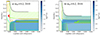 |
Fig. 8. Same as Fig. 6, but with 41Ca on the colour scale. |
| In the text | |
|
Fig. 9. Same as Fig. 5, but for 19F (left) and 22Ne (right). The lower panels show the ratio between the yield of the reference models (log(Denv/cm2 s−1) = 0) and the models with the other values for log(Denv/cm2 s−1). |
| In the text | |
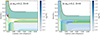 |
Fig. 10. Same as Fig. 6 but with 19F on the colour scale. |
| In the text | |
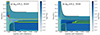 |
Fig. 11. Same as Fig. 6 but with 22Ne on the colour scale. |
| In the text | |
|
Fig. 12. Yields for the main isotopes of the CNO cycle for the different values of αov and log(Denv/cm2 s−1) (dots connected by lines). The horizontal lines indicate the yields of 20 M⊙ models (dashed, dashed-dotted, and dotted lines) with different rotational velocities (0, 150, and 300 km/s, from Brinkman (2022)). The isotopes are 12C, 13C, 14N, 15N, 16O, and in the last panel 17O (solid lines) and 18O (dash-dotted lines). In this panel, the grey horizontal lines are for 17O and the black horizontal lines are for 18O. The lower panels show the ratio between the yield of the reference models (log(Denv/cm2 s−1) = 0) and the models with the other values for log(Denv/cm2 s−1). |
| In the text | |
|
Fig. 13. Change of the C/N and N/O ratios on the surface of the models given at seven different times in the evolution; at the zero-age main sequence (ZAMS), half-way the main sequence (MMS), at the terminal-age main sequence (TAMS), on the Hertzsprung gap (HRG), and at the onset of helium burning (ZAHeB). The symbols are for the different values for αov while the colours indicate the different amounts of log(Denv/cm2 s−1) in the same way as in the previous figures. |
| In the text | |
|
Fig. 14. 14N abundance profiles at four different phases of the evolution of the models with αov = 0.2 and log(Denv/cm2 s−1) = 0 (blue) and 6 (purple). The top left panel shows the profiles halfway the main sequence (MMS), the top right at the end of the main sequence (TAMS), the bottom left at the beginning of the Hertzsprung gap (HRG), and the bottom right at the onset of helium burning (ZAHeB). The grey lines a (dashed for 0 km/s and dotted for 300 km/s) are from Brinkman (2022). |
| In the text | |
Current usage metrics show cumulative count of Article Views (full-text article views including HTML views, PDF and ePub downloads, according to the available data) and Abstracts Views on Vision4Press platform.
Data correspond to usage on the plateform after 2015. The current usage metrics is available 48-96 hours after online publication and is updated daily on week days.
Initial download of the metrics may take a while.