| Issue |
A&A
Volume 687, July 2024
|
|
|---|---|---|
| Article Number | A226 | |
| Number of page(s) | 15 | |
| Section | Planets and planetary systems | |
| DOI | https://doi.org/10.1051/0004-6361/202349082 | |
| Published online | 16 July 2024 | |
The GAPS programme at TNG
LVII. TOI-5076b: A warm sub-Neptune planet orbiting a thin-to-thick-disk transition star in a wide binary system★
1
INAF – Osservatorio Astrofisico di Catania,
Via Santa Sofia 78,
95123
Catania,
Italy
e-mail: This email address is being protected from spambots. You need JavaScript enabled to view it.
2
Dipartimento di Fisica e Astronomia “Ettore Majorana”, Università di Catania,
Via S. Sofia 64,
95123
Catania,
Italy
3
Scuola Superiore di Catania, Università di Catania,
Via Valdisavoia 9,
95123
Catania,
Italy
4
Department of Physics, University of Rome “Tor Vergata”,
Via della Ricerca Scientifica 1,
00133
Rome,
Italy
5
INAF – Osservatorio Astrofisico di Torino,
via Osservatorio 20,
10025
Pino Torinese,
Italy
6
Department of Physics, Engineering and Astronomy, Stephen F. Austin State University,
1936 North St,
Nacogdoches,
TX
75962,
USA
7
Cerro Tololo Inter-American Observatory,
Casilla 603,
La Serena,
Chile
8
Department of Physics and Astronomy, The University of North Carolina at Chapel Hill,
Chapel Hill,
NC 2599-3255,
USA
9
Sternberg Astronomical Institute of Lomonosov Moscow State University,
Moscow
119234,
Russia
10
INAF – Osservatorio Astronomico di Padova,
Vicolo dell’Osservatorio 5,
35122
Padova,
Italy
11
INAF – Osservatorio Astronomico di Roma,
Via Frascati 33,
00040
Monte Porzio Catone (RM),
Italy
12
Max Planck Institute for Astronomy,
Königstuhl 17,
69117
Heidelberg,
Germany
13
International Institute for Advanced Scientific Studies (IIASS),
Via G. Pellegrino 19,
84019
Vietri sul Mare (SA),
Italy
14
Dipartimento di Fisica e Astronomia “Galileo Galilei”, Università degli Studi di Padova,
Vicolo dell’Osservatorio 3,
35122
Padova,
Italy
15
INAF – Osservatorio Astronomico di Trieste,
via Tiepolo 11,
34143
Trieste,
Italy
16
Fundación Galileo Galilei–INAF,
Rambla José Ana Fernandez Pérez 7,
38712,
Breña Baja,
TF,
Spain
17
INAF – Osservatorio Astronomico di Palermo “G.S. Vaiana”,
Piazza del Parlamento 1,
90134
Palermo,
Italy
18
Department of Astrophysical Sciences, Princeton University,
Princeton,
NJ
08544,
USA
19
Department of Earth, Atmospheric and Planetary Sciences, Massachusetts Institute of Technology,
77 Massachusetts Avenue,
Cambridge,
MA
02139,
USA
20
Department of Physics and Kavli Institute for Astrophysics and Space Research, Massachusetts Institute of Technology,
Cambridge,
MA
02139,
USA
21
Department of Aeronautics and Astronautics, Massachusetts Institute of Technology,
77 Massachusetts Avenue,
Cambridge,
MA
02139,
USA
22
Center for Astrophysics | Harvard & Smithsonian,
60 Garden Street,
Cambridge,
MA
02138,
USA
23
University of Southern Queensland, Centre for Astrophysics,
West Street,
Toowoomba,
QLD 4350,
Australia
24
NASA Goddard Space Flight Center,
Greenbelt,
MD
20771,
USA
Received:
22
December
2023
Accepted:
19
April
2024
Abstract
Aims. We report the confirmation of a new transiting exoplanet orbiting the star TOI-5076.
Methods. We present our vetting procedure and follow-up observations which led to the confirmation of the exoplanet TOI-5076b. In particular, we employed high-precision TESS photometry, high-angular-resolution imaging from several telescopes, and high-precision radial velocities from HARPS-N.
Results. From the HARPS-N spectroscopy, we determined the spectroscopic parameters of the host star: Teff = (5070±143) K, log 𝑔 = (4.6±0.3), [Fe/H] = (+0.20±0.08), and [α/Fe] = 0.05±0.06. The transiting planet is a warm sub-Neptune with a mass mp = (16±2) M⊙, a radius rp =(3.2±0.l) R⊙ yielding a density ρp = (2.8±0.5) g cm−3. It revolves around its star approximately every 23.445 days.
Conclusions. The host star is a metal-rich, K2V dwarf, located at about 82 pc from the Sun with a radius of R⋆ = (0.78±0.01) R⊙ and a mass of M⋆ = (0.80±0.07) M⊙. It forms a common proper motion pair with an M-dwarf companion star located at a projected separation of 2178 au. The chemical analysis of the host-star and the Galactic-space velocities indicate that TOI-5076 belongs to the old population of thin-to-thick-disk transition stars. The density of TOI-5076b suggests the presence of a large fraction by volume of volatiles overlying a massive core. We found that a circular orbit solution is marginally favored with respect to an eccentric orbit solution for TOI-5076b.
Key words: techniques: photometric / techniques: radial velocities / planets and satellites: gaseous planets / binaries: visual / planets and satellites: general / planets and satellites: oceans
Full Tables 2 and 3 are available at the CDS via anonymous ftp to cdsarc.cds.unistra.fr (130.79.128.5) or via https://cdsarc.cds.unistra.fr/viz-bin/cat/J/A+A/687/A226
© The Authors 2024
 Open Access article, published by EDP Sciences, under the terms of the Creative Commons Attribution License (https://creativecommons.org/licenses/by/4.0), which permits unrestricted use, distribution, and reproduction in any medium, provided the original work is properly cited.
This article is published in open access under the Subscribe to Open model. This email address is being protected from spambots. You need JavaScript enabled to view it. to support open access publication.
1 Introduction
More than half of Sun-like stars host planets with radii in between the radius of the Earth and the one of Neptune (Howard et al. 2012; Fressin et al. 2013; Petigura et al. 2018; Zhu & Dong 2021). These sub-Neptune-sized objects (rp < 4R⊕) do not have analogs in our own Solar System and represent a new class of planets identified by exoplanet surveys. Observations from the NASA Kepler mission have demonstrated that the radius distribution of these objects presents a bimodality with a relative paucity of planets with radii between 1.5 R⊕ and 2 R⊕ (Fulton et al. 2017; Fulton & Petigura 2018; Van Eylen et al. 2018). This bimodality hints at some mechanisms that may have sculpted the observed radii distribution. Planets below the gap are currently interpreted as stripped cores that lost their atmospheres by means of certain physical processes such as photoevaporation (Owen & Wu 2013) or core-powered mass loss (Ginzburg et al. 2018), while planets above the radius gap were able to retain their atmospheres or are water worlds (Zeng et al. 2019). Increasing the sample of sub-Neptunes with precisely measured masses, radii, and densities found around different physical environments is important when it comes to clarifying the origins of this class of exoplanets.
It is still debated whether the birthplace of planets within the Milky Way plays an important role with regard to their orbital and physical properties. In the solar neighborhood, stars belong to three main populations: the thin disk, the thick disk, and the halo (Gilmore & Reid 1983). Thick-disk stars are considered to be older, kinematically hotter, metal-poorer, and more α-enhanced than thin-disk stars (e.g., Gilmore et al. 1989; Bensby et al. 2005; Adibekyan et al. 2012a; Recio-Blanco et al. 2014). Santos et al. (2017) suggested that planets belonging to different stellar populations, with different abundance ratios, may originate from planetary building blocks that have significantly different composition trends. For example, metal-poor thick-disk stars are expected to produce building blocks with much lower iron-mass fractions (which may imply smaller core masses) but higher water-mass fractions than thin-disk stars.
Bashi et al. (2020) provided first estimates of the occurrence rates of small close-in planets (2–100 days, 1–20 M⊕) for FGK dwarfs in the solar neighborhood thin and thick disks of the Galaxy. They found that the occurrence rates for planets in the two populations are, overall, comparable with the fraction of stars with planets  and the average number of planets per star np = 0.36±0.05. In the metal-poor regime ([Fe/H] < −0.25), however, Bashi et al. (2020) found a significantly larger occurrence rate of small close-in planets around high-α (thick disk) stars than around low-α (thin-disk) stars, while in the iron-rich region there seems to be almost no difference between the occurrence rates around thin- and thick-disk stars, though the sample of metal-rich, α-enhanced planet hosts is still too small to make any definite conclusion.
In this work, we report the confirmation of TOI-5076b, a warm sub-Neptune planet orbiting a nearby K2V star member of a binary system and part of the metal-rich, α-enhanced population of neighbor stars, with kinematics and chemistry that make it consistent with old, thin-to-thick-disk transition stars. These properties may provide important clues concerning the Galactic formation history of this star and of its planetary system (Adibekyan et al. 2011). This is also relevant considering that most transiting exoplanets have been discovered so far around thin-disk stars (e.g., Biazzo et al. 2022). Table 1 summarizes some properties of the target star.
This transiting planet was found using the data provided by the Transiting Exoplanet Survey satellite (TESS) (Ricker et al. 2015). The candidate exoplanet is reported in the Exo-FOP database1. TESS is a mission that was launched in April 2018 and observes the full sky searching for transiting planets around bright stars. The Global Architecture of Planetary Systems (GAPS, Naponiello et al. 2022) collaboration followed up this target with the High Accuracy Radial velocity Planet Searcher for the Northern hemisphere (HARPS-N) spectrograph (Cosentino et al. 2012). Additional high-angular resolution imaging observations from several observatories have been acquired to further investigate the target. We analyzed photometric and spectroscopic data simultaneously to infer the properties of the transiting body and of its host star.
In Sect. 2, we describe the photometric, high-angular-resolution imaging and spectroscopic observations we acquired. In Sect. 3, we describe our reduction procedure. In Sect. 4, we describe our vetting procedure of the planetary candidate. We describe the properties of the host star in Sect. 5 and the planetary properties in Sect. 6. In Sect. 7, we discuss our results, and in Sect. 8 we conclude our analysis.
2 Observations
2.1 Photometry
TOI-5076 was observed by TESS between August, 2021 and November, 2021. We used TESS full frame images (FFIs) to study this object. FFIs were calibrated by the TESS Science Processing Operations Center at NASA Ames Research Center (Jenkins et al. 2016). The TESS satellite imaged TOI-5076 during the fourth year of operation in three sectors: sector 42 (Camera 4, CCD 3), sector 43 (Camera 3, CCD 2), and sector 44 (Camera 1, CCD 4). Full frame images were acquired with a cadence of 10 min. In total, the satellite collected 10 220 images of the target. The first image was taken on August 21, 2021 at 04:29 UT and the last image on November 5, 2021 at 22:27 UT.
In total, four transits have been observed. Figure 1 shows the target pixel file (TPF) for TOI-5076 relative to the cadence 175 714 of sector 42. The image represents an area of ~3.5 square arcmin around the target. The red dots denote sources from Gaia DR3 corrected for proper motion at the TPF epoch. Their dimension is scaled inversely and proportionally to their difference in apparent Gaia G-band magnitude with respect to the target. We used a modified version of tpfplotter (Aller et al. 2020) to generate this figure.
Identifiers, astrometric and photometric measurements, and astrophysical properties of the host star.
2.2 High-angular-resolution imaging
2.2.1 SOAR
High-angular-resolution imaging is needed to search for nearby sources that can contaminate the TESS photometry, resulting in an underestimated planetary radius, or that may be the source of astrophysical false positives, such as background eclipsing binaries. We searched for stellar companions to TOI-5076 with speckle imaging on the 4.1-m Southern Astrophysical Research (SOAR) telescope (Tokovinin 2018) on November 4, 2022 UT, observing in Cousins I-band, a similar visible band pass to TESS. This observation was sensitive to a 4.9-magnitude-fainter star at an angular distance of 1 arcsec from the target. More details of the observations within the SOAR TESS survey are available in Ziegler et al. (2020). The 5σ detection sensitivity and speckle auto-correlation functions from the observations are shown in Fig. 2 (top). No nearby stars were detected within 3″ of TOI-5076 in the SOAR observations.
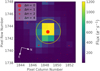 |
Fig. 1 TESS target pixel file (TPF) showing the position of TOI-5076 relative to the cadence 175 714 of sector 42. The image represents an area of ~3.5 square arcmin around the target. Sources in Gaia DR3 are represented by the red dots, scaled inversely proportionally to their difference of apparent G-band magnitude with respect to the target and corrected for proper motion to the epoch of the TPF. The yellow circle shows our adopted photometric aperture. |
2.2.2 WIYN
We used the NN-Explore Exoplanet Stellar Speckle Imager (NESSI, Scott et al. 2018) at the Wisconsin-Indiana-Yale-NOIRLab (WIYN) 3.5-m telescope to obtain high-resolution images of TOI-5076 on February 5, 2023 UT as part of the speckle imaging queue at WIYN. NESSI is a dual-channel imager that takes simultaneous image sets in two cameras at red and blue wavelengths. We used 40 nm wide filters with central wavelengths of 562 and 832 nm. The target was centered in a 256 × 256 pixel (4.6 × 4.6 arcsec) subregion of the CCDs and observed in a series of 9000, 40 ms frames at a plate scale near 0.018″/pixel in each camera. The TOI-5076 observations were followed by a 1000-frame observation of HD 23363 to serve as a point source calibrator. Additionally, during the queue run, various binary stars with well-established astrometric properties were observed to calibrate the instrument’s plate scales and orientations. The NESSI speckle data were reduced using a custom speckle data reduction pipeline described by Howell et al. (2011). This pipeline produces high-level data products including reconstructed images of the field around the target and contrast curves measured from those images. We did not detect any stellar companions brighter than ∆m = 4.85 and 5.79 at ρ = 1.2″ (and remaining constant out to 4.68 arcsec from the source) at 562 and 832 nm, respectively (where ρ is the separation from the source), as shown in Fig. 2 (middle).
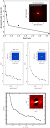 |
Fig. 2 High-angular-resolution imaging observations of the target. Top: speckle imaging obtained at 4.1-m Southern Astrophysical Research (SOAR) telescope. Middle: speckle imaging obtained at 3.5-m Wisconsin-Indiana-Yale-NOIRLab (WIYN) telescope. Bottom: speckle imaging obtained at 2.5-m telescope at the Caucasian Observatory of the Sternberg Astronomical Institute (SAI). |
2.2.3 SAI
TOI-5076 was observed on November 20, 2022 with the speckle polarimeter on the 2.5-m telescope at the Caucasian Observatory of Sternberg Astronomical Institute (SAI) of Lomonosov Moscow State University. The speckle polarime-ter uses high–speed low–noise CMOS detector Hamamatsu ORCA–quest (Strakhov et al. 2023). The atmospheric dispersion compensator was active, which allowed us to use the Ic band. The respective angular resolution is 0.083″, while the long-exposure atmospheric seeing was 0.6″. We did not detect any stellar companions brighter than ∆Ic = 3.8 and 6.2 at ρ = 0.25″ and 1.0″, respectively, where ρ is the separation between the source and the potential companion (Fig. 2, bottom).
2.3 Spectroscopy
2.3.1 TRES
Two spectra were obtained using the Tillinghast Reflector Echelle Spectrograph (TRES; Fűrész 2008) on January 21, 2022 and January 31, 2022 as part of the TESS Follow-up Observing Program2 Sub Group 1 (TFOP; Collins 2019) to check for false positive scenarios and determine stellar parameters.
During the first night, we obtained a spectrum with signal-to-noise ratio (S/N) = 25.4 and a radial velocity of RV = 71.145 km s−1. During the second night, we obtained S/N = 31.1 and RV = 71.087 km s−1. The two TRES observations yield a velocity offset of 58 m s−1 that was out of phase with the photometric ephemeris as reported in the ExoFOP observing notes3. TRES radial velocities were not used in the radial-velocity fit (Sect. 6).
TRES is mounted on the 1.5-m telescope atop the Fred Lawrence Whipple Observatory (FLWO) in Arizona. It operates in the spectral range of 390–910 nm, with a spectral resolution of R = 44000.
2.3.2 HARPS-N
Spectroscopic observations were obtained with the HARPS-N spectrograph at the Telescopio Nazionale Galileo (TNG) at the Observatorio del Roque de los Muchachos (La Palma). HARPS-N is an echelle spectrograph covering the wavelength range from 383 to 693 nm, with a spectral resolution R = 115 000, which allows radial-velocity measurements with the highest accuracy currently available in the northern hemisphere. We acquired 44 measurements with an exposure time of 15 min, 20 min, or 30 min within the context of the GAPS program. The observations were performed between August 16, 2022 and March 16, 2023.
3 Data analysis
3.1 Photometry
The TESS images were analyzed with the DIAmante pipeline following the procedure described in Montalto et al. (2020). In brief, the TESS FFIs were analyzed with a difference imaging approach where a stacked reference image was subtracted from each image after convolving the reference by an optimal kernel. The photometry was extracted using a circular aperture of radius equal to 2 pixels. We chose this aperture after testing different aperture radii between 1 pix and 4 pix and selecting the one with the smallest scatter. The light curves from different sectors were merged together by accounting for sector-by-sector photometric zero-point variations; then, they were corrected for systematics on a sector-by-sector basis by using a best set of eigen light curves extracted from the quietest and most highly correlated light curves in the same CCD where the target was observed (Montalto et al. 2020). To select the number of eigen light curves, we used the Akaike criterium, which indicated that three eigen light curves were appropriate. Finally, we normalized the light curve by a cubic spline function fitted on out-of-transit data with knots set every three hours. Table 2, available at CDS, presents the photometric measurements extracted by the pipeline. The first column indicates the time of observations at mid exposure (in BJDTDB), the second column the normalized flux (Flux), and the third column the error on the normalized flux (σFlux).
In Fig. 3, we show the light curve corrected for system-atics using eigen light curves (top) and the final splined light curve (bottom). We only analyzed the data that were not flagged by the pipeline (see Montalto et al. 2020) and that lie within a [+3σ, −5σ] interval between the mean of the normalized out-of-transit flux (9592 measurements). The transit analysis was further restricted to the measurements acquired between ± 10 hours from each transit event (721 measurements). As can be seen in Fig. 1, three faint sources are included in the photometric aperture. Because the difference imaging approach subtracts all the constant sources and because the reference flux of the target is calibrated from the TESS (TICv8.2, Paegert et al. 2022) magnitude derived from Gaia (where the target is resolved from the contaminating sources), no dilution correction is needed.
TESS photometric measurements of TOI-5076.
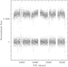 |
Fig. 3 Light curve obtained from TESS during different processing steps. Top: TESS light curve corrected for systematics with eigen light curves. Bottom: final light curve normalized by a spline fit on out-of-transit data. The light curves are offset vertically by +0.006 for clarity. |
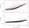 |
Fig. 4 BLS periodogram of systematics-corrected and splined light curve (top) and of the same light curve with transits subtracted (bottom). The dashed curves indicate the 1% false-alarm-probability (FAP) threshold. The red, vertical, dashed lines in the top panel denote the periods where the BLS power surpasses the threshold. |
3.2 Spectroscopy
The spectra of TRES were extracted following procedures outlined in Buchhave et al. (2010). The spectroscopic data of HARPS-N were reduced by the HARPS-N Data Reduction Software (DRS v3.7, Lovis & Pepe 2007) using a G2 template mask. The first three columns of Table 3 report the observation time at mid-exposure (in BJD), the radial velocities (RV in km s−1) and their errors (σRV in km s−1) and are available at CDS.
4 Vetting
TOI-5076.01 was subjected to preliminary vetting to establish its plausibility as a planetary candidate. We used the vetting procedure reported in Montalto et al. (2020) and Montalto (2023) in which a random-forest classifier was trained to distinguish between planetary candidates and other false positives such as eclipsing binaries and short-term sinusoidal variables. The classifier received in input features extracted from the TESS light curve and the box-least-squares (BLS, Kovács et al. 2002) peri-odogram. The BLS periodogram of the TOI-5076b systematics corrected and splined light curve (Fig. 3, bottom) is presented in Fig. 4 (top). The highest peak is found at 23.444 days and it corresponds to a S/N = 35.9 for the transits folded with the estimated period. After modeling and subtracting the 23.444-day signal, the BLS periodogram did not show any other significant features associated with plausible transit events (Fig. 4, bottom). The random-forest classifier calculated a probability (PRF) that the candidate is an exoplanet equal to PRF = 99.6% corresponding to a false positive rate <10−6. We also analyzed the centroid motion of the target during the transit events to establish if the transits were likely associated with the target star or to a star near the target. The centroid motion was analyzed in four concentric apertures between 1 pix and 4 pix, and two probabilities were derived: PD, the probability that the source of variability was associated with the target given the observed centroid motion measurements distributions and Pη, the reliability of the centroid motion results considering the local density of stars surrounding the target (Montalto et al. 2020; Montalto 2023). For TOI-5076, we obtained PD = 98% and Pη = 82%, which are both well above our adopted thresholds for acceptance (PD = 50% and Pη = 30%). Moreover, the algorithm also identified the star with the smallest Mahlanobis distance to the center of the distribution of centroid motion measurements of each aperture. For all tested apertures, we obtained that TOI-5076 was the star with the closest distance (RANK = 1 for all apertures) as depicted in Fig. 5. From this analysis, we concluded that TOI-5076.01 is a statistically validated exoplanet, and hereafter we name it TOI-5076b.
In Fig. 6 (top), we also present the generalized Lomb-Scargle (GLS; Zechmeister & Kürster 2009) periodogram of the HARPS-N radial-velocity measurements. The horizontal dashed line indicates the 1 % false alarm probability threshold obtained from 1000 bootstrap samples of the residual radial-velocity measurements. The highest peak of the HARPS-N radial-velocity measurements presents a GLS peak at 22.740 days, which is close to the period inferred from the global modeling (Table 4) and above the 1 % false-alarm threshold. We also note two peaks close to one day just above the 1% false-alarm-probability (FAP) threshold. However, after subtraction of the best-fit radialvelocity model (Sect. 6) the periodogram of the residual radialvelocity measurements (Fig. 6, bottom) does not present any significant peak above the 1% FAP threshold (as we already reported above for the analysis of the light curve residuals) indicating that no additional planets are detected in the data.
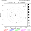 |
Fig. 5 Centroid motion analysis of TOI-5076. The target (at the center) and the surrounding stars are represented by black dots with diameters that are proportional to their Gaia DR3 magnitudes, as indicated by the legend on the right. All positions were corrected for proper motions to report them to the epoch of cadence 175714 of Sector 42. The figure also reports the TIC identification number and the Gaia DR3 source ID (in the top left and top right, respectively), the distributions of the calculated centroid motion measurements in each aperture (central colored ellipses), the Mahlanobis distance ranks, and the centroid motion probabilities (PD and Pη; see text). |
HARPS-N observations of TOI-5076.
5 Properties of the host star
5.1 Spectroscopic parameters
We measured the star’s effective temperature (Teff), surface gravity (log 𝑔), iron abundance [Fe/H], and microturbulence velocity (ξ) using the equivalent width method. We used the software StePar (Tabernero et al. 2019), which implements a grid of MARCS model atmospheres (Gustafsson et al. 2008) and the MOOG (Sneden 1973) radiative transfer code to compute stellar atmospheric parameters by means of a downhill simplex minimization algorithm, which minimizes a quadratic form composed of the excitation and ionization equilibrium of Fe. Equivalent widths were measured with ARES v2 (Sousa et al. 2015) from the coadded spectrum obtained from the individual HARPS-N spectra used for the radial-velocity measurements. The S/N of the coadded spectrum in the region between 5764 and 5766 Å measured using the ARES software was equal to S/N = 280. We used the FeI and FeII line list provided by the authors for the case of the Sun. Using this approach, we obtained the parameters reported in Table 1.
We also used the Stellar Parameter Classification tool (SPC, Buchhave et al. 2012) to derive stellar parameters using the TRES recon spectra and the average results from the two spectra (Teff = 4947 K ± 50 K, log 𝑔 = 4.54 ± 0.10, [m/H] = 0.23 ± 0.08, and υ sin i = 3 km s−1 ± 1 km s−1) agree with the results reported in Table 1.
We also note that, for TOI-5076, the Strömgren photometry is available in Hauck & Mermilliod (1998) which provide the following: (b-y) = 0.576, m1 = 0.589, c1 = 0.260. We corrected for reddening the photometry using E(B – V) = 0.005 obtained from our estimated extinction AV = 0.015 (Sect. 5.4) adopting a standard reddening law and the relations x0 = x − E(B − V) * kx where x = (b-y),m1,c1 and kx = 0.822,−0.319,0.176 are deduced from Árnadóttir et al. (2010). We then obtained (b-y)0 = 0.572, m10 = 0.591, c10 = 0.259. Adopting the calibration of Ramírez & Meléndez (2005), we obtained an estimated photometric metal-licity equal to [Fe/H] = +0.35. The estimated uncertainty on the metallicity derived from this photometric calibration is 0.2 dex (Ramírez & Meléndez 2005). Overall, this result agrees with the spectroscopic metallicity and confirms that the target is a metal-rich star.
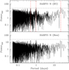 |
Fig. 6 GLS periodogram of HARPS-N radial-velocity measurements (top) and of the radial velocities measurements after subtraction of the best-fit radial-velocity model (bottom). The horizontal dashed line indicates the 1 % FAP threshold. The red, vertical, and dashed lines in the top panel denote the periods where the GLS power exceeds the FAP threshold. |
5.2 α-elements
Using the same radiative transfer code and model atmospheres as done for the determination of the stellar atmospheric parameters and iron abundance, and considering the line list by Biazzo et al. (2022), we measured the elemental abundances of the four α-elements Mg, Si, Ca, and Ti. Using these elements and the definition ![Mathematical equation: $[\alpha /{\rm{Fe}}] = {1 \over 4}([{\rm{Mg}}/{\rm{Fe}}] + [{\rm{Si}}/{\rm{Fe}}] + [{\rm{Ca}}/{\rm{Fe}}] + [{\rm{Ti}}/{\rm{Fe}}])$](/articles/aa/full_html/2024/07/aa49082-23/aa49082-23-eq4.png) , we obtain [α/Fe] = 0.05+0.064 for TOI-5076.
, we obtain [α/Fe] = 0.05+0.064 for TOI-5076.
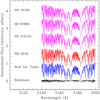 |
Fig. 7 Comparison of target spectrum in Mgb triplet region with empirical spectra in the Yee et al. (2017) library. The target’s spectrum is depicted in red. The three spectra of the library most highly correlated with the target’s spectrum are shown in magenta, while the best-fit linear combination of them is depicted in blue. The residuals between the target’s spectrum and the best fit are represented in black. |
5.3 Empirical spectral library
We also compared the spectroscopic parameters we derived in the previous section with the ones obtained using the spectra of the empirical library of Yee et al. (2017). This library includes 404 stars observed with Keck/HIRES by the California Planet Search. We used the software SpecMatch-Emp (Yee et al. 2017) to perform the comparison between our stacked spectrum of TOI-5076 and the library spectra. In Fig. 7, we represent the three empirical library spectra5 most highly correlated with the target spectrum in the region of the Mgb triplet in magenta. We indicate the target spectrum in red and the best-fit linear combination of the three reference spectra reported above in blue. Finally, at the bottom we show the difference between the target’s spectrum and the linearly combined reference spectra in black. In this case we obtained Teff = (4728±110) K, log 𝑔 = (4.5±0.1) dex, and [Fe/H] = (0.10±0.09) dex, which are all consistent within 2σ with the spectroscopic parameters previously derived and adopted.
5.4 Stellar parameters
We derived stellar parameters using Gaia DR3 (Riello et al. 2021), 2MASS (Skrutskie et al. 2006; Cohen et al. 2003), and ALLWISE (W1, W2, W3, and W4) photometry (Wright et al. 2010; Jarrett et al. 2011) together with the spectroscopic constraints obtained in Sect. 5. The effective temperature, the gravity, and the metallicity were constrained using a Gaussian prior and adopting the values reported in Table 1. We imposed a uniform prior on the distance, [d−3 × σd; d+3 × σd], where d = 82.78 pc was the distance obtained from the simple inversion of the parallax, and σd = 0.07 pc was the semi-difference between the upper and lower distance estimates obtained by subtracting and adding the parallax standard error from and to the Gaia DR3 parallax value. We also imposed a uniform prior on the interstellar extinction A550 (the monochromatic extinction at 550 nm). We first calculated the expected value of the monochromatic extinction (A550) for our target using the extinction map of Lallement et al. (2022). At the position of TOI-5076, we obtained A550 = (0.015±0.005). Then we considered the values between ![Mathematical equation: $\left[ {0;{A_{550}} + 3 \times {\sigma _{{A_{550}}}}} \right] = [0;0.030]$](/articles/aa/full_html/2024/07/aa49082-23/aa49082-23-eq5.png) as a plausible interval for the optical extinction.
as a plausible interval for the optical extinction.
The broadband photometry was obtained using the Padova library of stellar isochrones (PARSEC, Bressan et al. 2012). We generated a set of isochrones with an age (τ) comprised between τ = [107; 1010] yr and a logarithmic step size equal to log(Age) = 0.5. We varied the metallicity of the isochrone set between [M/H] = [− 2.0; 0.3] in steps of size equal to 0.05 dex. For each value of the effective temperature, gravity, and metal-licity generated by the algorithm, we identified the stellar model with the closest stellar parameters in our isochrone set. A small perturbation was applied to the effective temperature and the gravity to estimate the gradient of each quantity of interest (photometry and stellar parameters) with respect to these two parameters in a close surrounding of the identified model grid point, and a first-order Taylor expansion was applied to estimate any physical quantity of interest to the exact value of the simulated gravity and effective temperature. We then obtained the corresponding broadband absolute photometry and applied the distance modulus and extinction. To convert the monochromatic extinction (A550) to the extinction in any other photometric band (AX), we calculated the ratio (AX/A550) using a set of MARCS (Gustafsson et al. 2008) stellar spectra of dwarf stars for a broad range of effective temperatures and extinctions and interpolated the results for a star of Teff = 5070 K and a A550 = 0.01 5. We also calculated the parallax (from the simulated distance value).
We then compared these simulated values of the broadband photometry and of the parallax with the observed ones. The log-likelihood function we adopted to evaluate the model performance was equal to ln  , where oi and
  denote the observed magnitudes (and uncertainties) in different photometric bands and the measured parallax (and uncertainty), while the si are the corresponding simulated quantities. For any simulated model, we also registered the value of the stellar mass, stellar radius, luminosity, and age. To incorporate a systematic error component in our analysis, we also performed the fit using the set of BaSTI isochrones (Hidalgo et al. 2018) adding the differences of the best-fit parameters’ values obtained using, respectively, the Padova and BaSTI models in quadrature to the parameters’ uncertainties obtained using the Padova models.
The posterior distributions of the parameters were obtained using the nested sampling method implemented in the MultiNest package (Feroz & Hobson 2008; Buchner et al. 2014; Feroz et al. 2009, 2019). We used 250 live points. The result of the fit is shown in Fig. 8. The reduced chi-square of the fit (χr) is equal to Xr=1.16. The best-fit stellar mass and radius are M⋆ = (0.80±0.07) M⊙ and R⋆ = (0.78±0.01) R⊙, respectively. We also obtained a distance (d) equal to d = (82.8±0.1) pc, an extinction equal to AV = (0.015±0.009), and an age equal to τ = (9±6) Gyr. The results of our analysis are reported in Table 1.
Using the empirical spectral library described in Sect. 5.3, we also derived the stellar parameters obtaining R⋆ = (0.8±0.1) R⊙, M⋆ = (0.77±0.08) M⊙, and log Age = (12.5±5) Gyr, which are all consistent with our previous estimate. Moreover, the template spectra (Fig. 7) used to match the spectrum of TOI-5076 all have υ sin i = 1 km s−1. Such a value is at the limit of the HARPS-N resolution. The generalized Lomb-Scargle periodogram (GLS; Zechmeister & Kürster 2009) of the systematics-corrected out-of-transit data obtained by TESS (Fig. 9) has the highest peak at ~27.79 days. This is also close to the period of 33.4 days inferred from the activity index-rotation period relationship (see Sect. 5.7.1) of Astudillo-Defru et al. (2017). However, since the duration of a TESS sector is about 27 days, the observed modulation should be considered with care.
An alternative method to determine the stellar parameters is described in Montalto et al. (2021) and employed for the construction of the all-sky PLATO input catalog (as PIC1.1). In this case, we obtained Teff = (4867±206) K, R⋆ = (0.81±0.09) R⊙ and M⋆ = (0.79±0.07) M⊙. These estimates are all compatible with the parameters obtained by the Bayesian approach described in the first part of this section, which was finally adopted in our analysis along with the stellar parameters we derived.
System parameters relative to TOI-5076.
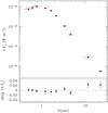 |
Fig. 8 Spectral energy distribution of the target obtained from broadband optical and near-infrared photometry. Top: optical and near-infrared broadband photometric measurements of the target star (black circles) and best-fit model (red open circles). Bottom: difference between logarithm of measurements and model’s estimates. |
5.5 Binarity
The host star forms a common proper motion pair with the close-by companion 2MASS J03220140+1714465 (Gaia DR3 55752974765291264) as reported in Gould & Chanamé (2004). Gaia DR3 supports such an association giving for the companion star µα = (168.20 ± 0.08) mas yr−1, µδ = (−175.41 ± 0.07) mas yr−1 and a parallax equal to π = (11.99 ± 0.07) which are consistent with the proper motions and parallax of TOI-5076 reported in Table 1. Using the Gaia DR3 color and the method described in Montalto et al. (2021), we deduced that the companion star has an effective temperature of Teff = (3115 ± 190) K and is a M 4.5V star. The companion is located at a parallactic angle equal to PA = 330.4° at a projected separation of 26.4 arcsec from TOI-5076, which corresponds to 2178 au.
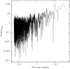 |
Fig. 9 Generalized Lomb-Scargle periodogram of systematics corrected out-of-transit data obtained by TESS. |
5.6 Galactic velocities
We used the kinematic approach of Bensby et al. (2003) to calculate the Galactic space velocities of TOI-5076 with respect to the local standard of rest (LSR) obtaining ULSR = −64.19 km s−1, VLSR = −74.69 km s−1, WLSR = −39.10 km s−1 and to estimate the probability that the host star belongs to the thin disk (Pthin), the thick disk (Pthick), and the halo (Phalo). For the probabilities, we obtained Pthin = 5.1%, Pthick = 94.8%, and Phalo = 0.1%. We therefore conclude that TOI-5076 is likely a thick-disk star from a kinematic point of view, and therefore it should be an old star with an age on the order of (10±5) Gyr (Bensby et al. 2003).
5.7 Stellar activity
5.7.1 Chromospheric activity
In Fig. 10 (top), we present the chromospheric activity index log  as a function of the radial-velocity measurements. To calculate this index, we used the YABI software deployed at IA2 Data-Center7. The Pearson correlation coefficient between the log
  index and the radial velocities is equal to 0.06 (p-value = 0.6997), indicating a negligible correlation between these two quantities. The average log
  is <log
  > = (−4.85±0.05). According to the classification proposed by Henry et al. (1996), TOI-5076 is inactive. In Fig. 11 (top), we present the chromospheric activity index log
  as a function of the radial-velocity residuals (calculated after subtraction of the best-fit radial-velocity model, Sect. 6). The Pearson correlation coefficient between the log
  index and the radial velocities is equal to 0.001 (p-value = 0.9938), indicating a negligible correlation between these two quantities.
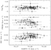 |
Fig. 10 Correlation between several activity indicators and the radial velocities. Top: chromospheric activity index log |

5.7.2 FWHM of the cross-correlation function
In Fig. 10 (middle), we present the FWHM of the cross-correlation function (CCF) as a function of the radial-velocity measurements. To calculate this index, we used the HARPS-N pipeline. The Pearson correlation coefficient between the FWHM index and the radial velocities is equal to −0.2546 (p-value = 0.0954), indicating a negligible correlation between these two quantities. In Fig. 11 (middle), we present the FWHM of the CCF as a function of the radial-velocity residuals. The Pearson correlation coefficient between the FWHM index and the radial-velocity residuals is equal to −0.2498 (p-value = 0.1019), indicating a negligible correlation between these two quantities.
5.7.3 Bisector span
In Fig. 10 (bottom), we report the bisector span (Queloz et al. 2001) versus the radial-velocity measurements. Such a quantity was calculated by the HARPS-N pipeline, and it is a measure of the line asymmetry, which may suggest the presence of issues related to activity and/or multiplicity. The error on the bisector has been assumed equal to twice the error on the radial velocities. We measured only a weak, not significant, positive correlation between the radial velocities and the bisector span (rparson = 0.3393, p-value = 0.02423). In Fig. 12, we show the periodogram of the bisector-span measurements and the false alarm probability threshold (FAP = 1 %) calculated from 1000 bootstrap resamples of the bisector-span measurements. No significant peak is observed.
In Fig. 11 (bottom), we report the bisector span versus the radial-velocity residuals. The Pearson correlation coefficient between the bisector span index and the radial-velocity residuals is equal to 0.2403 (p-value = 0.1161), indicating a negligible correlation between these two quantities. On the basis of these results, we conclude that stellar activity has a negligible impact on the observed radial velocities.
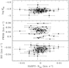 |
Fig. 11 Correlation between several activity indicators and radialvelocity residuals. Top: chromospheric activity index log |

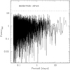 |
Fig. 12 Periodogram of bisector-span measurements and FAP threshold (FAP = 1%). |
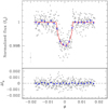 |
Fig. 13 Folded photometric measurements, the best-fit photometric model and residuals of the fit. Top: TESS light curve of TOI-5076 (gray points) folded with best-fit ephemerides. The best-fit transit model is denoted by the red curve. The point in the bottom left depicts the average uncertainty of the photometric measurements. Blue points represent measurements rebinned in 20 phase bins between the minimum and maximum phases. Bottom: residuals of fit. |
6 Planetary parameters
Planetary parameters were obtained by performing a simultaneous fit of both spectroscopic and photometric data with the juliet software (Espinoza et al. 2019). For the transiting planet, we assumed a Keplerian orbit, fixing the eccentricity to e = 0 and the argument of periastron to ω = 90°. To model the planet-to-star radius ratio p and the impact parameter b, we adopted the parametrization of Espinoza (2018). We sampled limb-darkening coefficients with the method described in Kipping (2013). We adopted uninformative priors for all parameters. Jitter parameters were adopted both for HARPS-N and for TESS data to absorb underestimated white-noise errors and unaccounted-for sources of red noise. In total, we fit 12 parameters reported in the top section of Table 4. The posterior distributions of the parameters were obtained using MultiNest via PyMultiNest (Buchner et al. 2014). We adopted 250 live points.
We also fit a Keplerian orbit with nonzero eccentricity by fitting the additional parameters  and
and  8. The result implied a log evidence of ln Ze = 2975.82 ± 0.03 against a log evidence for the case of circular orbit of ln Zc = 2976.3 ± 0.1. Consequently, the circular orbit was preferred with an odds ratio equal to exp(∆ ln Z) = exp(ln Zc − ln Ze) =1.6±0.2. The eccentric orbit implied an eccentricity e = (0.20 ± 0.09). The circular orbit solution is preferred in our analysis because of its formally better log evidence with respect to the eccentric orbit solution and the consistency of the eccentric orbit with a circular orbit solution within 2.2σ. We note that an eccentric orbit would imply a value for the stellar density equal to ρ⋆ = (2.1 ± 0.5) g cm−3 and consistent within 0.5-σ with the stellar density obtained from the estimation of the stellar mass and radius, which is equal to ρ⋆ = (2.4 ± 0.4) g cm−3 (Sect. 5.4). From the circular orbit solution, we obtained ρ⋆ = (1.4 ± 0.2) g cm−3 (Table 4), which is consistent within 2.2σ with the stellar density obtained from the estimation of the stellar mass and radius.
We obtained that the transiting body is a sub-Neptune planet with a mass mp = (16±2) M⊕ and a radius rp = (3.2±0.1) R⊕ yielding a density ρp = (2.8±0.5) g cm−3. The best-fit photometric and radial-velocity models are shown in Figs. 13 and 14, together with the photometric and radial-velocity measurements folded with the best-fit period.
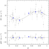 |
Fig. 14 Folded radial-velocity measurements, best-fit radial-velocity model and residuals of the fit. Top: HARPS-N radial-velocity measurements (gray points) folded with the best-fit orbital period and time of transit. The continuous line denotes the best-fit radial-velocity model. Blue points represent measurements rebinned in five phase bins. Bottom: residuals of fit. |
7 Discussion
The lack of correlation between the radial velocities and several activity indicators (Sect. 5.7) supports the Keplerian origin of the RV variations and the planetary nature of the transiting object. TOI-5076b is a sub-Neptune planet with a mass 10% smaller and a radius 16% smaller than Neptune. This yields a density about 1.5 times that of Neptune.
Weiss & Marcy (2014) studied the masses and radii of a sample of 65 exoplanets with radii of rp < 4 R⊕ and orbital periods of less than 100 days. They found that on average planets up to 1.5 R⊕ increase in density with increasing radius, indicating that their composition is mainly rocky. Planets with a radius of R > 1.5 R⊕ have average densities rapidly decreasing with increasing radius, suggesting that these planets have a large fraction of volatiles by volume overlying a rocky core. Moreover, they present a large compositional diversity of their atmospheres or rocky cores of different masses or compositions.
In Fig. 15, we present the average density versus planetary radius diagram of a sample of exoplanets, which we retrieved from the NASA exoplanet archive9. We only considered confirmed planets discovered either by the radial-velocity technique or the transit method and with radii smaller than 4 R ⊕. We imposed that both their radii and masses be determined with a precision level better than 20%. When multiple entries were present for the same planet, we used the default set of parameters adopted in the catalog by setting default_set=1. In total, the sample is composed of 165 exoplanets. The continuous lines in Fig. 15 represent the relationships defined in Weiss & Marcy (2014), where for planets with rp < 1.5 R⊕,
 (1)
(1)
while, for planets with 1.5 R⊕, ≤ rp < 4 R⊕,
 (2)
(2)
The position of TOI-5076b in this diagram is indicated by the green dot and it appears consistent with the decreasing branch of the planetary density versus planetary radius relationship defined by Eq. (2).
In Fig. 16, we present the planetary mass versus planetary radius diagram for the same sample of exoplanets of Fig. 15. Also in this case, the black continuous lines indicate the relationships of Weiss & Marcy (2014), and the position of TOI-5076b in this diagram is indicated by the green dot. In this case, Eq. (2) would predict mp = 7.9M⊕ for a radius equal to 3.2 R⊕, as does the one of TOI-5076b. The measured mass is instead mp = (16 ± 2) M⊕, which corresponds to 4.05 above the predicted value. We may argue that, since the host star is metal-rich (Table 1), there could have been favorable conditions for the accretion of a massive rocky core or for polluting the atmosphere of TOI-5076b with heavy elements. However, by looking at the sample of planets represented in Fig. 16, TOI-5076b is not an extremely massive sub-Neptune planet since several other planets with similar radii have masses beyond that of TOI-5076b.
We note that the presence of inflated planets could affect the radii and density distributions in Figs. 15 and 16. There are 17 planets with radii larger than our target in the sample we considered. Only four of them have an orbital period shorter than three days, and therefore they could be expected to have high equilibrium temperatures and potentially inflated atmospheres (the rest having orbital periods longer than six days). These are TOI-849b (Armstrong et al. 2020), TOI-2196b (Persson et al. 2022), TOI-132b (Díaz et al. 2020), and Kepler-94b (Marcy et al. 2014). All these planets have the fact that they lie in the so-called Neptune desert in common (Mazeh et al. 2016), which origin is still debated in the literature. These objects could possess extended atmospheres (as in the case of Kepler-94b) or could be the remnant cores of gas-giant planets (e.g., TOI-849b), or maybe the results of other complex evolutionary patterns. In any case, we note that the different evolutionary histories of these planets could affect their radii and therefore could slightly influence the Weiss & Marcy (2014) relations and change the relative position of those models with respect to our target position. However, this does not alter our conclusion that TOI-5076b is not an extremely massive sub-Neptune planet since the mass of these planets is not significantly affected by the inflation or envelope mass-loss mechanism.
In Fig. 17, we show the radius versus mass diagram for the sample of 165 planets discussed above (gray points) with a superimposed representative set of mass–radius models for planets with identical composition10. The position of TOI-5076b in this diagram seems more compatible with models with an H2 envelope, such as the model with a 49.95% Earth-like rocky core and a 49.95% H2O layer and 0.1% H2 envelope by mass represented by the red curve rather than models that have a pure composition of only one element.
In Sect. 5.5, we reported that the host star belongs to a binary system where the companion lies at a projected separation of 2178 au from the target. Such a wide binary likely does not significantly affect the architecture of a planetary system around one of its components (a so-called S-type configuration) as shown by statistical studies of planetary systems around wide (a > 100300 au) and close binaries, apart from the average eccentricity, which appears larger for planets in binary systems (both close and wide) than for planets around single stars (e.g., Su et al. 2021). Some hints that the orbit of TOI-5076b could be eccentric come from the fact that the circular orbit solution implies a rather low stellar density in comparison to the theoretical stellar density expected from stellar models, whereas the stellar density obtained assuming an eccentric orbit is higher and more consistent with the stellar model’s estimation, as we note in Sect. 6.
Using the [α/Fe] versus [Fe/H] positions as chemical indicators ofstellarpopulation(Fig. 18), TOI-5076appearstobelongto the region populated by α-enhanced and metal-rich stellar populations (Adibekyan et al. 2011; Bensby et al. 2014) and is close to the transition region between low- and high-α-content stars (dot-dashed line in Fig. 18).
This result, together with the values of the Galactic-space velocities and the high thick-to-thin disk probability reported in Sect. 5.6 seem to be consistent with the possible belonging of TOI-5076 to the old population of thin-to-thick-disk transition stars with relatively hot kinematics (e.g., see Fig. 20 in Bensby et al. 2014). This is also apparent in Fig. 19, where we present the Boettlinger and Toomre diagrams (top left and right, respectively) of the sample of planet host stars hosting at least one exoplanet with rp < 4R⊕ (and for which a precision level in the estimation of planetary masses and radii better than 20% was achieved). This sample was retrieved from the NASA exoplanet archive, and it was matched with the Gaia DR3 catalog from which we extracted the positions, proper motions, and radial velocities of the host stars. The distances were taken from the NASA exoplanet archive. In total, the sample amounts to 112 stars11. With these quantities, we calculated the Galactic velocities (Bensby et al. 2003) reported in the diagrams ofFig. 19. ThepositionofTOI-5076b(blueopentriangle) appears peripheral in these diagrams, indicating that the velocity of TOI-5076b is relatively high with respect to the velocities of the sample of stars studied here. In the bottom row of Fig. 19, we present the probability distributions that the same sample of stars belong to the thin disk (bottom left), the thick disk (bottom in the middle), and to the halo (bottom right). Most of the stars are likely members of the thin disk. Only 10% of these stars have a probability >90% (as TOI-5076b) of belonging to the thick disk, while all of them have a negligible probability of belonging to the halo.
The planet’s equilibrium temperature (Teq) can be estimated with
 (3)
(3)
where a is the orbital semi-major axis, R* the stellar radius, T* the host star’s effective temperature, and A the Bond albedo12. We obtained Teq = (615 ± 20) K.
Assuming an H2-dominated solar-abundance atmosphere, the scale height of the planetary atmosphere is  , where kb is the Boltzmann constant, Teq is the planet’s equilibrium temperature, µ = 2.3 amu is the mean molecular weight, and 𝑔 is the gravity. For TOI-5076b we have H = 142 km, while the amplitude of spectral features in transmission for a clear atmosphere is ~ 4pH/R* = 39 ppm (Kreidberg 2018), where p is the radius ratio and R* is the radius of the star.
We also calculated the transmission spectroscopy metric (TSM; Kempton et al. 2018) to understand the suitability of this target for transmission spectroscopy using the James Webb Space Telescope (JWST). The TSM parameter provides an estimate of the S/N reachable in a 10 h observing program using JWST/NIRISS, and it is defined as
 (4)
(4)
where S is a normalization constant to match the more detailed work of Louie et al. (2018), Rp is the radius of the planet in units of Earth radii, Mp is the mass of the planet in units of Earth masses, R* is the radius of the host star in units of solar radii, mJ is the apparent magnitude of the host star in the J band, and Teq is the equilibrium temperature expressed in Kelvin. From Table 1 of Kempton et al. (2018), we chose S = 1.28 considering the radius of TOI-5076b. We found a value of TSM = 29. This places TOI-5076b in the fourth quartile of the TSM values of the statistical sample of planets simulated by Kempton et al. (2018) and is below the suggested cut-off value (TSM = 84) for follow-up efforts.
Therefore, the atmospheric characterization of TOI-5076b can be considered challenging in comparison with other more favorable targets. We could also discuss tentative trends identified in the small sample of warm Neptunes studied so far (Crossfield & Kreidberg 2017), which suggests that both Teq and fHHe (H and He mass fractions, which can be traced by rp) play a key role in setting the amplitude of the H2O absorption feature at 1.4 µm in transmission spectroscopy. The relatively low equilibrium temperature13 (Teq = 581 K) of TOI-5076b would fall below the threshold identified by Crossfield & Kreidberg (2017) for the formation of hazes in the atmosphere of warm Neptunes (Teq = 850 K). Therefore, most or all transmission features should be blocked in TOI-5076b. While the density of TOI-5076b is compatible with the presence of an H/He envelope (see Fig. 15), its relatively large mass (Fig. 16) could suggest a massive rocky core and/or a metal-rich atmosphere (as we note above), which would also decrease the amplitude of atmospheric features in transmission.
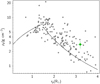 |
Fig. 15 Planetary density versus planetary radius for sample of planets with R < 4 R⊕ described in the text. The black continuous lines denote the relations of Weiss & Marcy (2014). The position of TOI-5076b in this diagram is indicated by the green dot. |
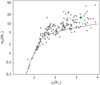 |
Fig. 16 Planetary mass versus planetary radius for sample of planets with R < 4 R⊕ described in the text. The black continuous lines denote the relations of Weiss & Marcy (2014). The position of TOI-5076b in this diagram is indicated by the green dot. |
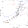 |
Fig. 17 Radii and masses of exoplanets with rP < 4 R⊕ discussed in the text (gray points). The position of TOI-5076b in this diagram is shown by the black dot. We also represent the position ofNeptune (blue dot). The colored and continuous lines denote mass-radius models for planets with the same composition. In particular: pure iron (100% Fe, brown curve); Earth-like rocky (32.5% Fe+67.5% MgSiO3, magenta); pure rock (100% MgSiO3, black curve); pure water (100% H2O, blue curve);0.1%H2envelope(49.95%Earth-likerockycore+49.95%H2O layer + 0.1% H2 envelope by mass), assuming 1 milli-bar surface pressure level and isothermal atmosphere at 700K (red curve). |
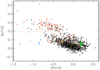 |
Fig. 18 [alpha/Fe] vs. [Fe/H] for TOI-5076 (star symbol). Thin-disk, thick-disk, and halo field stars as in Adibekyan et al. (2012b) are shown with circles, squares, and asterisks, respectively. The crosses refer to their thin-thick and thick-halo transition stars. The dot-dashed line separates the stars with high-and low-alpha content as derived by the same authors. |
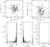 |
Fig. 19 Boettlinger (top left) and Toomre (top right) diagrams for the sample of planet host stars (black dots) described in the text. The position of TOI-5076b is marked by the open blue triangle. In the bottom row are depicted the probability distributions to belong to the thin disk (bottom left), the thick disk (bottom middle) and the halo (bottom right). The vertical blue lines denote the probabilities for TOI-5076b. |
8 Conclusions
In this work, we report the confirmation of a new transiting exoplanet orbiting the star TOI-5076. Using HARPS-N spec-troscopy, we determined that the host star is a metal-rich K2V dwarf located about 82 pc from the Sun with a radius of R⋆ = (0.78±0.01) R⊙ and a mass of M⋆ = (0.80±0.07) M⊙. It forms a common proper motion pair with an M-dwarf companion star located at a projected separation of 2178 au. The chemical analysis of the host star and the Galactic-space velocities indicate that TOI-5076 belongs to the old population of thin-to-thick-disk transition stars.
The transiting planet is a warm (Teq = 614±20 K) subNeptune with a mass of mp = (16±2) M⊕, and a radius of rp = (3.2±0.1) R⊕ yielding a density of ρp = (2.8±0.5) g cm−3. Its orbital period is 23.445 days.
The density of TOI-5076b suggests the presence of a large fraction by volume of volatiles overlying a massive core. We find that a circular orbit solution is marginally favored with respect to an eccentric orbit solution for TOI-5076b with the present data. In the case of the eccentric orbit solution, we obtained e = (0.20±0.09). The analysis of the photometric measurements and radial velocities after subtraction of the best-fit model do not show the presence of any additional planet in the system.
Acknowledgements
Based on observations made with the Italian Telescopio Nazionale Galileo (TNG) operated by the Fundación Galileo Galilei (FGG) of the Istituto Nazionale di Astrofisica (INAF) at the Observatorio del Roque de los Muchachos (La Palma, Canary Islands, Spain). This paper made use of data collected by the TESS mission and are publicly available from the Mikulski Archive for Space Telescopes (MAST) operated by the Space Telescope Science Institute (STScI). Funding for the TESS mission is provided by NASA’s Science Mission Directorate. We acknowledge the use of public TESS data from pipelines at the TESS Science Office and at the TESS Science Processing Operations Center. Resources supporting this work were provided by the NASA High-End Computing (HEC) Program through the NASA Advanced Supercomputing (NAS) Division at Ames Research Center for the production of the SPOC data products. This work made use of tpfplotter by J. Lillo-Box (publicly available in http://www.github.com/jlillo/tpfplotter), which also made use of the python packages astropy, lightkurve, matplotlib and numpy. This research has made use of the Exoplanet Follow-up Observation Program (ExoFOP; DOI: 10.26134/ExoFOP5) website, which is operated by the California Institute of Technology, under contract with the National Aeronautics and Space Administration under the Exoplanet Exploration Program. Some of the observations in the paper made use of the NN-EXPLORE Exoplanet and Stellar Speckle Imager (NESSI). NESSI was funded by the NASA Exoplanet Exploration Program and the NASA Ames Research Center. NESSI was built at the Ames Research Center by Steve B. Howell, Nic Scott, Elliott P. Horch, and Emmett Quigley. B.S.S. and I.A.S. acknowledge the support of M.V. Lomonosov Moscow State University Program of Development. T.Z.i. acknowledges NVIDIA Academic Hardware Grant Program for the use of the Titan V GPU card and the support by the CHEOPS ASI-INAF agreement n. 2019-29-HH.0 and the Italian MUR Departments of Excellence grant 2023-2027 “Quantum Frontiers”.
References
- Adibekyan, V. Z., Santos, N. C., Sousa, S. G., & Israelian, G. 2011, A&A, 535, L11 [NASA ADS] [CrossRef] [EDP Sciences] [Google Scholar]
- Adibekyan, V. Z., Santos, N. C., Sousa, S. G., et al. 2012a, A&A, 543, A89 [NASA ADS] [CrossRef] [EDP Sciences] [Google Scholar]
- Adibekyan, V. Z., Sousa, S. G., Santos, N. C., et al. 2012b, A&A, 545, A32 [NASA ADS] [CrossRef] [EDP Sciences] [Google Scholar]
- Aller, A., Lillo-Box, J., Jones, D., Miranda, L. F., & Barceló Forteza, S. 2020, A&A, 635, A128 [NASA ADS] [CrossRef] [EDP Sciences] [Google Scholar]
- Armstrong, D. J., Lopez, T. A., Adibekyan, V., et al. 2020, Nature, 583, 39 [Google Scholar]
- Árnadóttir, A. S., Feltzing, S., & Lundström, I. 2010, A&A, 521, A40 [NASA ADS] [CrossRef] [EDP Sciences] [Google Scholar]
- Astudillo-Defru, N., Delfosse, X., Bonfils, X., et al. 2017, A&A, 600, A13 [NASA ADS] [CrossRef] [EDP Sciences] [Google Scholar]
- Bashi, D., Zucker, S., Adibekyan, V., et al. 2020, A&A, 643, A106 [NASA ADS] [CrossRef] [EDP Sciences] [Google Scholar]
- Bensby, T., Feltzing, S., & Lundström, I. 2003, A&A, 410, 527 [CrossRef] [EDP Sciences] [Google Scholar]
- Bensby, T., Feltzing, S., Lundström, I., & Ilyin, I. 2005, A&A, 433, 185 [NASA ADS] [CrossRef] [EDP Sciences] [Google Scholar]
- Bensby, T., Feltzing, S., & Oey, M. S. 2014, A&A, 562, A71 [NASA ADS] [CrossRef] [EDP Sciences] [Google Scholar]
- Biazzo, K., D’Orazi, V., Desidera, S., et al. 2022, A&A, 664, A161 [NASA ADS] [CrossRef] [EDP Sciences] [Google Scholar]
- Bressan, A., Marigo, P., Girardi, L., et al. 2012, MNRAS, 427, 127 [NASA ADS] [CrossRef] [Google Scholar]
- Buchhave, L. A., Bakos, G. Á., Hartman, J. D., et al. 2010, ApJ, 720, 1118 [NASA ADS] [CrossRef] [Google Scholar]
- Buchhave, L. A., Latham, D., Johansen, A., et al. 2012, Nature, 486, 375 [NASA ADS] [CrossRef] [Google Scholar]
- Buchner, J., Georgakakis, A., Nandra, K., et al. 2014, A&A, 564, A125 [NASA ADS] [CrossRef] [EDP Sciences] [Google Scholar]
- Cohen, M., Wheaton, W. A., & Megeath, S. T. 2003, AJ, 126, 1090 [Google Scholar]
- Collins, K. 2019, AAS Meeting Abstracts, 233, 140.05 [NASA ADS] [Google Scholar]
- Cosentino, R., Lovis, C., Pepe, F., et al. 2012, SPIE Conf. Ser., 8446, 84461V [Google Scholar]
- Crossfield, I. J. M., & Kreidberg, L. 2017, AJ, 154, 261 [Google Scholar]
- Díaz, M. R., Jenkins, J. S., Gandolfi, D., et al. 2020, MNRAS, 493, 973 [Google Scholar]
- Espinoza, N. 2018, Res. Notes Am. Astron. Soc., 2, 209 [Google Scholar]
- Espinoza, N., Kossakowski, D., & Brahm, R. 2019, MNRAS, 490, 2262 [Google Scholar]
- Feroz, F., & Hobson, M. P. 2008, MNRAS, 384, 449 [NASA ADS] [CrossRef] [Google Scholar]
- Feroz, F., Hobson, M. P., & Bridges, M. 2009, MNRAS, 398, 1601 [NASA ADS] [CrossRef] [Google Scholar]
- Feroz, F., Hobson, M. P., Cameron, E., & Pettitt, A. N. 2019, Open J. Astrophys., 2, 10 [Google Scholar]
- Fűrész, G. 2008, PhD thesis, University of Szeged, Hungary [Google Scholar]
- Fressin, F., Torres, G., Charbonneau, D., et al. 2013, ApJ, 766, 81 [NASA ADS] [CrossRef] [Google Scholar]
- Fulton, B. J., & Petigura, E. A. 2018, AJ, 156, 264 [Google Scholar]
- Fulton, B. J., Petigura, E. A., Howard, A. W., et al. 2017, AJ, 154, 109 [Google Scholar]
- Gaia Collaboration (Vallenari, A., et al.) 2023, A&A, 674, A1 [NASA ADS] [CrossRef] [EDP Sciences] [Google Scholar]
- Gilmore, G., & Reid, N. 1983, MNRAS, 202, 1025 [Google Scholar]
- Gilmore, G., Wyse, R. F. G., & Kuijken, K. 1989, ARA&A, 27, 555 [NASA ADS] [CrossRef] [Google Scholar]
- Ginzburg, S., Schlichting, H. E., & Sari, R. 2018, MNRAS, 476, 759 [Google Scholar]
- Gould, A., & Chanamé, J. 2004, ApJS, 150, 455 [CrossRef] [Google Scholar]
- Gustafsson, B., Edvardsson, B., Eriksson, K., et al. 2008, A&A, 486, 951 [NASA ADS] [CrossRef] [EDP Sciences] [Google Scholar]
- Hauck, B., & Mermilliod, M. 1998, A&AS, 129, 431 [NASA ADS] [CrossRef] [EDP Sciences] [Google Scholar]
- Henry, T. J., Soderblom, D. R., Donahue, R. A., & Baliunas, S. L. 1996, AJ, 111, 439 [Google Scholar]
- Hidalgo, S. L., Pietrinferni, A., Cassisi, S., et al. 2018, ApJ, 856, 125 [Google Scholar]
- Howard, A. W., Marcy, G. W., Bryson, S. T., et al. 2012, ApJS, 201, 15 [Google Scholar]
- Howell, S. B., Everett, M. E., Sherry, W., Horch, E., & Ciardi, D. R. 2011, AJ, 142, 19 [Google Scholar]
- Jarrett, T. H., Cohen, M., Masci, F., et al. 2011, ApJ, 735, 112 [Google Scholar]
- Jenkins, J. M., Twicken, J. D., McCauliff, S., et al. 2016, Proc. SPIE, 9913, 99133E [Google Scholar]
- Kempton, E. M. R., Bean, J. L., Louie, D. R., et al. 2018, PASP, 130, 114401 [Google Scholar]
- Kipping, D. M. 2013, MNRAS, 435, 2152 [Google Scholar]
- Kovács, G., Zucker, S., & Mazeh, T. 2002, A&A, 391, 369 [Google Scholar]
- Kreidberg, L. 2018, Handbook of Exoplanets, eds. H. J. Deeg, & J. A. Belmonte (Springer International Publishing AG), 100 [Google Scholar]
- Lallement, R., Vergely, J. L., Babusiaux, C., & Cox, N. L. J. 2022, A&A, 661, A147 [NASA ADS] [CrossRef] [EDP Sciences] [Google Scholar]
- Louie, D. R., Deming, D., Albert, L., et al. 2018, PASP, 130, 044401 [NASA ADS] [CrossRef] [Google Scholar]
- Lovis, C., & Pepe, F. 2007, A&A, 468, 1115 [NASA ADS] [CrossRef] [EDP Sciences] [Google Scholar]
- Marcy, G. W., Isaacson, H., Howard, A. W., et al. 2014, ApJS, 210, 20 [NASA ADS] [CrossRef] [Google Scholar]
- Mazeh, T., Holczer, T., & Faigler, S. 2016, A&A, 589, A75 [NASA ADS] [CrossRef] [EDP Sciences] [Google Scholar]
- Montalto, M. 2023, MNRAS, 518, L31 [Google Scholar]
- Montalto, M., Borsato, L., Granata, V., et al. 2020, MNRAS, 498, 1726 [NASA ADS] [CrossRef] [Google Scholar]
- Montalto, M., Piotto, G., Marrese, P. M., et al. 2021, A&A, 653, A98 [NASA ADS] [CrossRef] [EDP Sciences] [Google Scholar]
- Naponiello, L., Mancini, L., Damasso, M., et al. 2022, A&A, 667, A8 [NASA ADS] [CrossRef] [EDP Sciences] [Google Scholar]
- Owen, J. E., & Wu, Y. 2013, ApJ, 775, 105 [Google Scholar]
- Paegert, M., Stassun, K. G., Collins, K. A., et al. 2021, arXiv e-prints [arXiv: 2108.04778] [Google Scholar]
- Paegert, M., Stassun, K. G., Collins, K. A., et al. 2022, VizieR Online Data Catalog: IV/39 [Google Scholar]
- Pecaut, M. J., & Mamajek, E. E. 2013, ApJS, 208, 9 [Google Scholar]
- Persson, C. M., Georgieva, I. Y., Gandolfi, D., et al. 2022, A&A, 666, A184 [NASA ADS] [CrossRef] [EDP Sciences] [Google Scholar]
- Petigura, E. A., Marcy, G. W., Winn, J. N., et al. 2018, AJ, 155, 89 [Google Scholar]
- Queloz, D., Henry, G. W., Sivan, J. P., et al. 2001, A&A, 379, 279 [NASA ADS] [CrossRef] [EDP Sciences] [Google Scholar]
- Ramírez, I., & Meléndez, J. 2005, ApJ, 626, 446 [Google Scholar]
- Recio-Blanco, A., de Laverny, P., Kordopatis, G., et al. 2014, A&A, 567, A5 [NASA ADS] [CrossRef] [EDP Sciences] [Google Scholar]
- Ricker, G. R., Winn, J. N., Vanderspek, R., et al. 2015, J. Astron. Telesc. Instrum. Syst., 1, 014003 [Google Scholar]
- Riello, M., De Angeli, F., Evans, D. W., et al. 2021, A&A, 649, A3 [NASA ADS] [CrossRef] [EDP Sciences] [Google Scholar]
- Santos, N. C., Adibekyan, V., Dorn, C., et al. 2017, A&A, 608, A94 [NASA ADS] [CrossRef] [EDP Sciences] [Google Scholar]
- Scott, N. J., Howell, S. B., Horch, E. P., & Everett, M. E. 2018, PASP, 130, 054502 [Google Scholar]
- Skrutskie, M. F., Cutri, R. M., Stiening, R., et al. 2006, AJ, 131, 1163 [NASA ADS] [CrossRef] [Google Scholar]
- Sneden, C. 1973, ApJ, 184, 839 [Google Scholar]
- Sousa, S. G., Santos, N. C., Adibekyan, V., Delgado-Mena, E., & Israelian, G. 2015, A&A, 577, A67 [NASA ADS] [CrossRef] [EDP Sciences] [Google Scholar]
- Strakhov, I. A., Safonov, B. S., & Cheryasov, D. V. 2023, Astrophys. Bull., 78, 234 [NASA ADS] [CrossRef] [Google Scholar]
- Su, X.-N., Xie, J.-W., Zhou, J.-L., & Thebault, P. 2021, AJ, 162, 272 [NASA ADS] [CrossRef] [Google Scholar]
- Tabernero, H. M., Marfil, E., Montes, D., & Gonzalez Hernandez, J. I. 2019, A&A, 628, A131 [NASA ADS] [CrossRef] [EDP Sciences] [Google Scholar]
- Tokovinin, A. 2018, PASP, 130, 035002 [Google Scholar]
- Van Eylen, V., Agentoft, C., Lundkvist, M. S., et al. 2018, MNRAS, 479, 4786 [Google Scholar]
- Weiss, L. M., & Marcy, G. W. 2014, ApJ, 783, L6 [Google Scholar]
- Wright, E. L., Eisenhardt, P. R. M., Mainzer, A. K., et al. 2010, AJ, 140, 1868 [Google Scholar]
- Yee, S. W., Petigura, E. A., & von Braun, K. 2017, ApJ, 836, 77 [Google Scholar]
- Zechmeister, M., & Kürster, M. 2009, A&A, 496, 577 [CrossRef] [EDP Sciences] [Google Scholar]
- Zeng, L., Jacobsen, S. B., Sasselov, D. D., et al. 2019, Proc. Natl. Acad. Sci., 116, 9723 [Google Scholar]
- Zhu, W., & Dong, S. 2021, ARA&A, 59, 291 [NASA ADS] [CrossRef] [Google Scholar]
- Ziegler, C., Tokovinin, A., Briceño, C., et al. 2020, AJ, 159, 19 [Google Scholar]
As claimed by Adibekyan et al. (2011), for [Fe/H] > 0 the [Ca/Fe] trend for dwarf stars in the Galactic disk differs from that of Mg, Si, and Ti. Also excluding this element for the [α/Fe] computation, we obtain [α/Fe] = (0.06±0.06), which is consistent with the value obtained considering all four elements.
The spectra of stars HD 16160, HD 87883, and HD 219134.
We added an error of 0.01 mag in quadrature to the Gaia broadband photometric errors reported in Table 1.
We adopted a uniform prior U(−0.89; 0.89) for both of them.
All models were taken from https://lweb.cfa.harvard.edu/~lzeng/planetmodels.html
A few stars for which no systemic radial velocity was found neither in the Gaia or NASA catalogs nor in the literature were eliminated.
We assumed here full heat redistribution and zero Bond albedo.
To be consistent with Crossfield & Kreidberg (2017), we assumed full heat redistribution and Bond albedo A = 0.2 here.
All Tables
Identifiers, astrometric and photometric measurements, and astrophysical properties of the host star.
All Figures
|
Fig. 1 TESS target pixel file (TPF) showing the position of TOI-5076 relative to the cadence 175 714 of sector 42. The image represents an area of ~3.5 square arcmin around the target. Sources in Gaia DR3 are represented by the red dots, scaled inversely proportionally to their difference of apparent G-band magnitude with respect to the target and corrected for proper motion to the epoch of the TPF. The yellow circle shows our adopted photometric aperture. |
| In the text | |
|
Fig. 2 High-angular-resolution imaging observations of the target. Top: speckle imaging obtained at 4.1-m Southern Astrophysical Research (SOAR) telescope. Middle: speckle imaging obtained at 3.5-m Wisconsin-Indiana-Yale-NOIRLab (WIYN) telescope. Bottom: speckle imaging obtained at 2.5-m telescope at the Caucasian Observatory of the Sternberg Astronomical Institute (SAI). |
| In the text | |
|
Fig. 3 Light curve obtained from TESS during different processing steps. Top: TESS light curve corrected for systematics with eigen light curves. Bottom: final light curve normalized by a spline fit on out-of-transit data. The light curves are offset vertically by +0.006 for clarity. |
| In the text | |
|
Fig. 4 BLS periodogram of systematics-corrected and splined light curve (top) and of the same light curve with transits subtracted (bottom). The dashed curves indicate the 1% false-alarm-probability (FAP) threshold. The red, vertical, dashed lines in the top panel denote the periods where the BLS power surpasses the threshold. |
| In the text | |
|
Fig. 5 Centroid motion analysis of TOI-5076. The target (at the center) and the surrounding stars are represented by black dots with diameters that are proportional to their Gaia DR3 magnitudes, as indicated by the legend on the right. All positions were corrected for proper motions to report them to the epoch of cadence 175714 of Sector 42. The figure also reports the TIC identification number and the Gaia DR3 source ID (in the top left and top right, respectively), the distributions of the calculated centroid motion measurements in each aperture (central colored ellipses), the Mahlanobis distance ranks, and the centroid motion probabilities (PD and Pη; see text). |
| In the text | |
|
Fig. 6 GLS periodogram of HARPS-N radial-velocity measurements (top) and of the radial velocities measurements after subtraction of the best-fit radial-velocity model (bottom). The horizontal dashed line indicates the 1 % FAP threshold. The red, vertical, and dashed lines in the top panel denote the periods where the GLS power exceeds the FAP threshold. |
| In the text | |
|
Fig. 7 Comparison of target spectrum in Mgb triplet region with empirical spectra in the Yee et al. (2017) library. The target’s spectrum is depicted in red. The three spectra of the library most highly correlated with the target’s spectrum are shown in magenta, while the best-fit linear combination of them is depicted in blue. The residuals between the target’s spectrum and the best fit are represented in black. |
| In the text | |
|
Fig. 8 Spectral energy distribution of the target obtained from broadband optical and near-infrared photometry. Top: optical and near-infrared broadband photometric measurements of the target star (black circles) and best-fit model (red open circles). Bottom: difference between logarithm of measurements and model’s estimates. |
| In the text | |
|
Fig. 9 Generalized Lomb-Scargle periodogram of systematics corrected out-of-transit data obtained by TESS. |
| In the text | |
|
Fig. 10 Correlation between several activity indicators and the radial velocities. Top: chromospheric activity index log |
| In the text | |
|
Fig. 11 Correlation between several activity indicators and radialvelocity residuals. Top: chromospheric activity index log |
| In the text | |
|
Fig. 12 Periodogram of bisector-span measurements and FAP threshold (FAP = 1%). |
| In the text | |
|
Fig. 13 Folded photometric measurements, the best-fit photometric model and residuals of the fit. Top: TESS light curve of TOI-5076 (gray points) folded with best-fit ephemerides. The best-fit transit model is denoted by the red curve. The point in the bottom left depicts the average uncertainty of the photometric measurements. Blue points represent measurements rebinned in 20 phase bins between the minimum and maximum phases. Bottom: residuals of fit. |
| In the text | |
|
Fig. 14 Folded radial-velocity measurements, best-fit radial-velocity model and residuals of the fit. Top: HARPS-N radial-velocity measurements (gray points) folded with the best-fit orbital period and time of transit. The continuous line denotes the best-fit radial-velocity model. Blue points represent measurements rebinned in five phase bins. Bottom: residuals of fit. |
| In the text | |
|
Fig. 15 Planetary density versus planetary radius for sample of planets with R < 4 R⊕ described in the text. The black continuous lines denote the relations of Weiss & Marcy (2014). The position of TOI-5076b in this diagram is indicated by the green dot. |
| In the text | |
|
Fig. 16 Planetary mass versus planetary radius for sample of planets with R < 4 R⊕ described in the text. The black continuous lines denote the relations of Weiss & Marcy (2014). The position of TOI-5076b in this diagram is indicated by the green dot. |
| In the text | |
|
Fig. 17 Radii and masses of exoplanets with rP < 4 R⊕ discussed in the text (gray points). The position of TOI-5076b in this diagram is shown by the black dot. We also represent the position ofNeptune (blue dot). The colored and continuous lines denote mass-radius models for planets with the same composition. In particular: pure iron (100% Fe, brown curve); Earth-like rocky (32.5% Fe+67.5% MgSiO3, magenta); pure rock (100% MgSiO3, black curve); pure water (100% H2O, blue curve);0.1%H2envelope(49.95%Earth-likerockycore+49.95%H2O layer + 0.1% H2 envelope by mass), assuming 1 milli-bar surface pressure level and isothermal atmosphere at 700K (red curve). |
| In the text | |
|
Fig. 18 [alpha/Fe] vs. [Fe/H] for TOI-5076 (star symbol). Thin-disk, thick-disk, and halo field stars as in Adibekyan et al. (2012b) are shown with circles, squares, and asterisks, respectively. The crosses refer to their thin-thick and thick-halo transition stars. The dot-dashed line separates the stars with high-and low-alpha content as derived by the same authors. |
| In the text | |
|
Fig. 19 Boettlinger (top left) and Toomre (top right) diagrams for the sample of planet host stars (black dots) described in the text. The position of TOI-5076b is marked by the open blue triangle. In the bottom row are depicted the probability distributions to belong to the thin disk (bottom left), the thick disk (bottom middle) and the halo (bottom right). The vertical blue lines denote the probabilities for TOI-5076b. |
| In the text | |
Current usage metrics show cumulative count of Article Views (full-text article views including HTML views, PDF and ePub downloads, according to the available data) and Abstracts Views on Vision4Press platform.
Data correspond to usage on the plateform after 2015. The current usage metrics is available 48-96 hours after online publication and is updated daily on week days.
Initial download of the metrics may take a while.