| Issue |
A&A
Volume 687, July 2024
|
|
|---|---|---|
| Article Number | A61 | |
| Number of page(s) | 20 | |
| Section | Extragalactic astronomy | |
| DOI | https://doi.org/10.1051/0004-6361/202348095 | |
| Published online | 27 June 2024 | |
The COSMOS-Web ring: In-depth characterization of an Einstein ring lensing system at z ∼ 2
1
Aix Marseille Univ, CNRS, CNES, LAM, Marseille, France
e-mail: wilfried.mercier@lam.fr
2
Cosmic Dawn Center (DAWN), Denmark
3
Niels Bohr Institute, University of Copenhagen, Jagtvej 128, 2200 Copenhagen, Denmark
4
Institut d’Astrophysique de Paris, UMR 7095, CNRS, Sorbonne Université, 98 bis boulevard Arago, 75014 Paris, France
5
Institute for Computational Cosmology, Durham University, South Road, Durham DH1 3LE, UK
6
DTU Space, Technical University of Denmark, Elektrovej, Building 328, 2800 Kgs. Lyngby, Denmark
7
Caltech/IPAC, 1200 E. California Blvd, Pasadena, CA 91125, USA
8
The University of Texas at Austin, 2515 Speedway Blvd Stop C1400, Austin, TX 78712, USA
9
Instituto de Astrofísica de Canarias (IAC), La Laguna 38205, Spain
10
Observatoire de Paris, LERMA, PSL University, 61 avenue de l’Observatoire, 75014 Paris, France
11
Université Paris-Cité, 5 Rue Thomas Mann, 75014 Paris, France
12
Universidad de La Laguna. Avda. Astrofísico Fco, Sanchez, La Laguna, Tenerife, Spain
13
Institute for Astronomy, University of Hawaii, 2680 Woodlawn Drive, Honolulu, HI 96822, USA
14
Department of Astronomy and Astrophysics, University of California, Santa Cruz, 1156 High Street, Santa Cruz, CA 95064, USA
15
Institute of Cosmology and Gravitation, University of Portsmouth, PO13FX Portsmouth, UK
16
Centre for Extragalactic Astronomy, Durham University, South Road, Durham DH1 3LE, UK
17
Department of Physics and Astronomy, University of Hawaii, Hilo, 200 W Kawili St, Hilo, HI 96720, USA
18
Center for Computational Astrophysics, Flatiron Institute, 162 Fifth Avenue, New York, NY 10010, USA
19
Department of Physics, Faculty of Science, University of Helsinki, 00014 Helsinki, Finland
20
Department of Computer Science, Aalto University, PO Box 15400, Espoo 00076, Finland
21
Technical University of Munich, TUM School of Natural Sciences, Department of Physics, James-Franck-Str. 1, 85748 Garching, Germany
22
Max-Planck-Institut für Astrophysik, Karl-Schwarzschild-Str. 1, 85748 Garching, Germany
23
University of California Santa Barbara, Santa Barbara, CA, USA
24
Jet Propulsion Laboratory, California Institute of Technology, 4800 Oak Grove Drive, Pasadena, CA 91109, USA
25
Laboratory for Multiwavelength Astrophysics, School of Physics and Astronomy, Rochester Institute of Technology, 84 Lomb Memorial Drive, Rochester, NY 14623, USA
26
Space Telescope Science Institute, 3700 San Martin Drive, Baltimore, MD 21218, USA
27
Kapteyn Astronomical Institute, University of Groningen, PO Box 800, 9700AV Groningen, The Netherlands
28
University of Bologna – Department of Physics and Astronomy “Augusto Righi” (DIFA), Via Gobetti 93/2, 40129 Bologna, Italy
29
INAF – Osservatorio di Astrofisica e Scienza dello Spazio, Via Gobetti 93/3, 40129 Bologna, Italy
30
Niels Bohr Institute, University of Copenhagen, Jagtvej 128, 2200 Copenhagen, Denmark
Received:
27
September
2023
Accepted:
20
February
2024
Aims. We provide an in-depth analysis of the COSMOS-Web ring, an Einstein ring at z ≈ 2 that we serendipitously discovered during the data reduction of the COSMOS-Web survey and that could be the most distant lens discovered to date.
Methods. We extracted the visible and near-infrared photometry of the source and the lens from more than 25 bands. We combined these observations with far-infrared detections to study the dusty nature of the source and we derived the photometric redshifts and physical properties of both the lens and the source with three different spectral energy distribution (SED) fitting codes. Using JWST/NIRCam images, we also produced two lens models to (i) recover the total mass of the lens, (ii) derive the magnification of the system, (iii) reconstruct the morphology of the lensed source, and (iv) measure the slope of the total mass density profile of the lens.
Results. We find the lens to be a very massive elliptical galaxy at z = 2.02 ± 0.02 with a total mass within the Einstein radius of Mtot(<θEin = (3.66 ± 0.36) × 1011 M⊙ and a total stellar mass of M⋆ = 1.37−0.11+0.14 × 10¹¹ M⊙. We also estimate it to be compact and quiescent with a specific star formation rate below 10−13 yr. Compared to stellar-to-halo mass relations from the literature, we find that the total mass of the lens within the Einstein radius is consistent with the presence of a dark matter (DM) halo of total mass Mh = 1.09−0.57+1.46 × 10¹³ M⊙. In addition, the background source is a M⋆ = (1.26 ± 0.17) × 1010 M⊙ star-forming galaxy (SFR ≈ (78 ± 15) M⊙ yr) at z = 5.48 ± 0.06. The morphology reconstructed in the source plane shows two clear components with different colors. Dust attenuation values from SED fitting and nearby detections in the far infrared also suggest that the background source could be at least partially dust-obscured.
Conclusions. We find the lens at z ≈ 2. Its total, stellar, and DM halo masses are consistent within the Einstein ring, so we do not need any unexpected changes in our description of the lens such as changing its initial mass function or including a non-negligible gas contribution. The most likely solution for the lensed source is at z ≈ 5.5. Its reconstructed morphology is complex and highly wavelength dependent, possibly because it is a merger or a main sequence galaxy with a heterogeneous dust distribution.
Key words: gravitation / gravitational lensing: strong / galaxies: distances and redshifts / galaxies: elliptical and lenticular, cD / galaxies: halos / galaxies: high-redshift
© The Authors 2024
 Open Access article, published by EDP Sciences, under the terms of the Creative Commons Attribution License (https://creativecommons.org/licenses/by/4.0), which permits unrestricted use, distribution, and reproduction in any medium, provided the original work is properly cited.
This article is published in open access under the Subscribe to Open model. Subscribe to A&A to support open access publication.
1. Introduction
Lensing happens whenever a light ray from a background galaxy is deviated toward the observer by a foreground mass distribution, including galaxy clusters (e.g., Lynds & Petrosian 1986; Soucail et al. 1987; Kneib et al. 1996; Campusano et al. 2001; Jauzac et al. 2015; Massey et al. 2018; Richard et al. 2021; Claeyssens et al. 2022; Atek et al. 2023) and massive galaxies (e.g., Walsh et al. 1979; Jauncey et al. 1991; Dye et al. 2014; Nightingale et al. 2023; Etherington et al. 2023). Depending on the alignment between the lens and the background source, as well as the shape of the lens’ potential, strong lensing can either produce multiple images of the same source (e.g., an Einstein cross, Huchra et al. 1985), gravitational arcs (e.g., Soucail et al. 1987), or a full Einstein ring (e.g Jauncey et al. 1991). Strong lensing is a powerful tool to study the properties of galaxies for two main reasons. First, it magnifies the flux of the background galaxy, allowing the detection of intrinsically fainter and/or higher redshift sources. In addition, this magnification enhances the resolution of the background source, allowing spatially resolved studies to be undertaken on small structures such as star-forming clumps (e.g., Swinbank et al. 2007, 2009; Jones et al. 2010; Livermore et al. 2012, 2015; Johnson et al. 2017a,b; Meštrić et al. 2022; Claeyssens et al. 2023). Second, the magnification and the shape of the gravitational arcs or rings are primarily impacted by the mass distribution of the lens. Therefore, lensing is one of the few observations along with galaxy dynamics allowing the total mass content of galaxies to be constrained, including hidden components such as their dark matter (DM) halo (e.g., Treu 2010; Oguri et al. 2014; Nightingale et al. 2023; Bolamperti et al. 2023).
For instance, this led to the discovery of the so-called ‘bulge-halo conspiracy’ where the total density profile (i.e., baryons + dark matter) of local early-type galaxies (ETGs) exhibit a nearly isothermal behavior (Gavazzi & Soucail 2007; Auger et al. 2010; Etherington et al. 2023). Samples up to zlens ∼ 0.8 further reveal varying trends in the value of the density profile slope γ with increasing zlens, from a mild decrease (Sonnenfeld et al. 2013) to a more significant increase (Bolton et al. 2012). Furthermore, cosmological simulations suggest a slight rise in γ with redshift (Wang et al. 2019, 2020), which are dependent on feedback mechanisms such as active galactic nuclei. However, our current understanding of the evolution of the density profiles of ETGs with redshift faces a limitation due to the scarcity of lenses identified at z ≳ 0.8.
While initially relatively rare, galaxy-galaxy lensing candidates have now become ubiquitous thanks to large and deep imaging surveys in the optical and near-infrared (NIR) such as in the Subaru Hyper Suprime-Cam (HSC) survey (e.g., Wong et al. 2018), the Hubble Space Telescope (HST) observations of the COSMOS field (e.g., Koekemoer et al. 2007; Faure et al. 2008a,b; Jackson 2008; Pourrahmani et al. 2018), the Dark Energy Survey (DES, e.g., Diehl et al. 2017; Rojas et al. 2022; O’Donnell et al. 2022), the Sloan Digital Sky Survey (SDSS, e.g., Auger et al. 2010; Talbot et al. 2021, 2022), the ASTRO 3D Galaxy Evolution with Lenses (AGEL) survey (Tran et al. 2022), the entire HST archives (Garvin et al. 2022), or in the radio with the Cosmic Lens All-Sky Survey (CLASS, e.g., Myers et al. 2003; Browne et al. 2003), the Herschel Multi-tiered Extragalactic Survey (HerMES, Wardlow et al. 2013), the Herschel Astrophysical Terahertz Large Area Survey (Herscel-ATLAS, e.g., Negrello et al. 2010, 2017), or using the South Pole Telescope (SPT, e.g., Vieira et al. 2010; Hezaveh & Holder 2011; Hezaveh et al. 2013; Vieira et al. 2013). Currently, the largest catalogs contain up to a few hundred excellent galaxy-galaxy lenses, and this effort was made possible thanks to the numerous developments brought to automatic lens detection algorithms (e.g., Gavazzi et al. 2014; Petrillo et al. 2017; Pourrahmani et al. 2018; Sonnenfeld et al. 2020; Cañameras et al. 2020, 2023; Savary et al. 2022).
Throughout the last decade, serendipitous discoveries and case-by-case studies of lenses have been pushed toward higher redshifts. So far, the highest redshift lenses ever discovered correspond to those of Cañameras et al. (2017) and Ciesla et al. (2020) both at z ≈ 1.5 and Wong et al. (2014) at z ≈ 1.6. But a new era is beginning for strong lensing with the advent of James Webb Space Telescope (JWST). Already, NIRCam and/or NIRISS observations of lensing clusters, such as Abell 2744 (e.g., see Bergamini et al. 2023; Bezanson et al. 2022) or SMACS0723 (e.g., see Atek et al. 2023), have detected multiple background sources at z > 9 (e.g., Bergamini et al. 2023; Atek et al. 2023). Complementarily, NIRSpec observations have allowed the spectroscopic confirmation of multiple galaxies at z ≳ 10 (e.g., Williams et al. 2023; Wang et al. 2023; Hsiao et al. 2023). Besides JWST, upcoming new telescopes and facilities with dedicated wide surveys will also play a crucial role in greatly improving the number of detected strong lenses. For instance, roughly 17 000 lenses are predicted in the Nancy Grace Roman Space Telescope 2000 square degree survey (see Sect. 12.2 and Fig. 12.7 of Weiner et al. 2020), on the order of 120 000 in the Vera C. Rubin Observatory Legacy Survey of Space and Time (LSST, see Sect.6 and beyond of Collett 2015), and between 95 000 (see Sect. 4.4 of Holloway et al. 2023) and 170 000 (Collett 2015) in the Euclid wide survey.
While such surveys will slightly extend the redshift range of strong lenses, very few are actually predicted to be discovered at z > 2 (e.g., see Fig. 6 of Collett 2015). Recently, Holloway et al. (2023) released an in-depth estimation of the detectability of strong lenses in the near-infrared (NIR), including JWST surveys such as the JWST Advanced Deep Extragalactic Survey (JADES) and COSMOS-Web. From purely source-lens alignment considerations, lenses could theoretically be detected up to z ∼ 4 (Holloway et al. 2023)1. However, when accounting for the magnification and shear of the source, the spatial resolution of JWST, and the limiting depth of the surveys, the predicted maximum redshift for lens detection is not predicted to exceed z ∼ 2, except in the case of extraordinary cases that will be more likely to happen in ultra-deep pencil-beam surveys such as JADES (see Fig. 5a of Holloway et al. 2023).
In this paper, we report the serendipitous discovery of the potentially highest redshift lens ever detected at z ∼ 2. The system was observed during data reduction of the COSMOS-Web survey in April 2023 and was unambiguously identified as an Einstein ring thanks to the high-resolution optical rest-frame images provided by JWST in multiple bands. While preparing this paper, van Dokkum et al. (2024) published an independent analysis of this system (dubbed named JWST-ER1). In this paper, we provide an in-depth analysis of the lens and the source by
-
(i)
Combining HST and JWST data with ground-based observations to constrain precisely the photometric redshift and physical properties of the lens and the source,
-
(ii)
Performing state-of-the-art mass modeling to constrain precisely the total mass of the lens and study its DM content,
-
(iii)
Reconstruct the morphology of the lensed source and
-
(iv)
Studying the dusty nature of the source using complementary FIR-to-radio detections.
We begin by presenting in Sect. 2 the observations of the system and the photometry used for the analysis. Then, we discuss the two lens models fitted on the observations in Sect. 3. In Sect. 4, we present the photometric redshift estimate and physical properties of both the source and the lens and in Sect. 5 we provide a discussion on
-
(i)
The mass budget of the foreground lens,
-
(ii)
The current constraints on the slope of the total mass profile of the lens,
-
(iii)
The possibility that the background source is made of multiple galaxies at different redshifts but aligned along the line-of-sight, and
-
(iv)
The dusty nature of the source.
Finally, we conclude in Sect. 6.
Throughout this paper, we adopt a standard ΛCDM cosmology with H0 = 70 km s−1 Mpc−1, Ωm = 0.3, and ΩΛ = 0.7. Physical parameters are estimated assuming a Chabrier (2003) initial mass function (IMF). The magnitudes are expressed in the AB system (Oke 1974).
2. Observations
2.1. COSMOS-Web ground- and space-based observations
The COSMOS-Web ring was discovered thanks to the JWST/NIRCam imaging of the COSMOS field as part of the COSMOS-Web survey (GO #1727), described in detail in Casey et al. (2023). Briefly, it consists of 255-hour imaging of a contiguous 0.54 deg2 area in four NIRCam filters (F115W, F150W, F277W, and F444W), down to a 5σ depth of AB mag 27.2 − 28.2, measured in empty apertures of 0.15″ radius (Casey et al. 2023). The NIRCam data reduction was carried out using the version 1.10.0 of the JWST Calibration Pipeline (Bushouse et al. 2022), Calibration Reference Data System (CRDS) pmap-1075 and a NIRCam instrument mapping imap-0252. Mosaics are created on both 30 mas and 60 mas pixel scales for all filters. The NIRCam image processing and mosaic making will be described in detail in Franco et al. (in prep.). COSMOS-Web offers a unique combination of area, depth, and NIRCam2 resolution to carry out searches for distant strong lensing systems. In this paper, we used the available data from COSMOS-Web at the time, which was only about 50% of the total area, imaged over two epochs (January 2023 and April 2023).
We complemented the JWST imaging with the wealth of existing ground-based and HST/ACS data, described in detail in Shuntov et al. (in prep.; see also Weaver et al. 2022 and Dunlop 2016). We summarize below the dataset used for our work. The u band imaging comes from the CFHT Large Area U-band Deep Survey (CLAUDS; Sawicki et al. 2019), reaching 27.7 mag (5σ). The ground-based optical imaging is provided by the HSC Subaru Strategic Program (HSC-SSP; Aihara et al. 2018). We used the HSC-SSP DR3 (Aihara et al. 2022) in the ultra-deep HSC imaging region in five g, r, i, z, y broad bands and three narrow bands, with a sensitivity ranging 26.5–28.1 mag (5σ). In addition, we included the reprocessed Subaru Suprime-Cam images with 12 medium bands in optical (Taniguchi et al. 2007, 2015). The UltraVISTA survey (McCracken et al. 2012) provides deep NIR imaging in four broad bands YJHKs and one narrow band (1.18 μm). Our source falls in one of the ultra-deep stripes of DR5 (Dunlop 2016). While being at a lower resolution and less sensitive than NIRCam, these data are complementary in terms of wavelength coverage. Finally, we also included the HST/ACS F814W band (Koekemoer et al. 2007) providing a high-resolution image in the i-band.
In order to constrain the dust-obscured star-forming activity of the ring (see Sect. 5.4), we adopted the deblended FIR photometry in the latest “Super-deblended” catalog of Jin et al. (in prep.; see also Jin et al. 2018 for a detailed description of the technique). From this catalog, we used measurements at MIPS 24 μm, Herschel PACS 100 μm and 160 μm, Herschel SPIRE 250 μm, 350 μm, and 500 μm (with conservative lower limits of confusion noise used for the SPIRE bands; see Nguyen et al. 2010), and SCUBA-2 850 μm which were obtained by performing the ‘Super-deblending’ technique (Jin et al. 2018; Liu et al. 2018) with priors from the COSMOS2020 catalog (Weaver et al. 2022). We note that the ring is not selected by COSMOS2020 due to its faintness. The only prior adopted for the deblending is on the position of the foreground lens. Given that the size of the ring is approximately 2″, it is not resolved in any of the FIR images mentioned above (e.g., see SCUBA-2 contours in Fig. A.1). Therefore, it is appropriate to use the position of the lens as a prior to deblend the FIR emission from other nearby sources.
2.2. Overview of the Einstein ring
Upon reduction of the JWST/NIRCam images of COSMOS-Web in April 2023, the COSMOS-Web ring was clearly identified by visual inspection at the coordinates RA = 150.10048° and Dec = 1.89301°. An RGB color image of the system produced by combining PSF-matched HST and JWST cutouts is shown in Fig. 1. The foreground lens is surrounded by the Einstein ring that shows strong inhomogeneities in color. Cutouts of the system in two JWST/NIRCam bands are shown in the leftmost column of Fig. 2 (see also Fig. A.4 for cutouts in all ground- and space-based bands). The morphology of the ring strongly varies with wavelength. This includes CW (clump west) and CE (clump east) that are detected mostly in the F277W and F444W bands, as well as a blue component that is visible throughout the ring, but in particular in its northern and southern parts. The latter looks quite smooth in the F277W and F444W bands but it becomes clumpy in the F814W, F115W, and F150W bands. Another galaxy is also located roughly 1.2″ south west of the ring and is estimated with LEPHARE (Arnouts et al. 2002; Ilbert et al. 2006) to be at z = 2.1 ± 0.1. Therefore, this galaxy could potentially be a satellite of the lens, in which case it would be located at around 10 ± 0.1 kpc away from it3. Finally, a last UV-bright galaxy, only visible in u, g, and r bands is visible west of the ring (see Fig. A.4). The fact that it is not seen near CE suggests that it is not part of the ring.
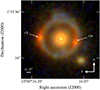 |
Fig. 1. False color image of the COSMOS-Web ring made by cutouts from the HST/ACS F814W, JWST/NIRCam F115W, and F150W bands into the blue channel, the NIRCam F277W band into the green channel and the NIRCam F444W band into the red channel. The white bar in the bottom left represents the PSF FWHM in the F444W band. Two clumps CW and CE in the ring are identified in the figure. North is up and east is to the left. |
Besides HST and JWST images, the system is also detected in all UltraVISTA bands, as well as in the HSC-i, z, and y bands. It is interesting to note that the component of the ring that is visible in these bands corresponds to the northern blue part. On the other hand, CW and CE do not appear at all. Starting from and blue-ward of the r-band, the whole system becomes a dropout. Assuming it corresponds to the Lyman break for the background source, it would place it at 4.5 ≲ zdrop ≲ 6.5. The lack of detection for the central lens blue-ward of the r-band is likely the combination of an intrinsic drop of the spectrum at these wavelengths combined with a coarser spatial resolution4 since the CFHT-u band is technically deeper than the HSC-g, r, and i bands.
When cross-correlating the position of the Einstein ring with strong-lensing catalogs that overlap with the COSMOS field, including that from Faure et al. (2008b), Pourrahmani et al. (2018), Wong et al. (2018), Sonnenfeld et al. (2018, 2020), and Garvin et al. (2022), we do not find any source that matches this system. The combination of its dropout nature at low wavelengths and the coarse spatial resolution of the ground-based observations certainly prevented its identification. Still, it is interesting to note that the lens and the ring are clearly visible and can be separated in the HST/ACS F814W band if the image is properly rescaled to enhance its contrast, and as such, it could have been detected in previous visual searches of strong-lensing candidates in the COSMOS field. Only the JWST/NIRCam images provide enough signal-to-noise ratio (S/N) to unambiguously identify this system as an Einstein ring. Similarly, JWST/NIRCam images are mandatory if one wants to derive precise photometric redshifts of both the lens and the source.
2.3. Photometry
We have used two sets of photometry to estimate the redshifts and galaxy properties of this system. The first one (noted SE++ hereafter) was derived using the SOURCEXTRACTOR++ software (Bertin et al. 2020; Kümmel et al. 2020). Four objects in this system were extracted from the full COSMOS-Web catalog (Shuntov et al., in prep.): the lens, the potential satellite, and the two clumps CW and CE. We modeled each object assuming their surface brightness follows a single Sérsic profile. The structural parameters (center position, Sérsic index n, radius, and axis ratio) are constrained using high-resolution HST and NIRCam images. For other bands (e.g., ground-based), only the flux of each object was allowed to vary during the fit. The fluxes of the four objects were fitted simultaneously, which is necessary when the objects are blended (e.g., the clumps and the lens in ground-based images). For each band, the profiles were convolved with the appropriate point spread function (PSF). The PSF models for all bands were built with PSFEX (Bertin 2011), by first running SEXTRACTOR to detect sources and select stars based on a FWHM vs. S/N criterion. As a validation and quality control, we compared the encircled energy profiles of our PSF models to those of real stars as measured in the images. The latter were selected as unsaturated stars in the Gaia DR3 star catalog. The size of the models was chosen such that it encompasses more than 99% of the encircled energy compared to those of real stars.
The second set of photometry was obtained from the lens modeling (hereafter SL_FIT photometry) performed with SL_FIT (see Sect. 3.1). The morphology of the foreground lens was modeled with a circular Sérsic profile with a fixed index n = 3, whereas the background source was best modeled in source plane with three Sérsic profiles with a fixed index n = 1 that do not share the same center. The structural parameters (center position and radius for the lens; center position, radius, and ellipticity for three components of the source) were determined from JWST/NIRCam images only. Only the flux of each component was allowed to vary when fitting other bands and, as for SE++ photometry, the appropriate PSF was taken into account for each band during the fit. Examples of SL_FIT and SE++ photometry extraction for JWST/NIRCam F444W and F115W bands are shown in Fig. 2. For the photometry of the background source, we summed the flux of the three components modeled by SL_FIT, unless stated otherwise.
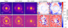 |
Fig. 2. Morphology of the COSMOS-Web ring in the F444W (top row) and F115W (bottom row) bands. From left to right: 3″ × 3″ cutouts, best-fit lens model in image plane from SL_FIT, best-fit morphological model of the lens, CW, CE, and the nearby satellite with SOURCEXTRACTOR++, residuals from SL_FIT, and residuals from SOURCEXTRACTOR++. For each band, the same flux scale is applied for the both image and the models. All images have been projected on the same HST coordinate grid (north up and east left) with a scale of 0.06″ per pixel. In both F115W and F444W images, the critical line from SL_FIT’s best-fit mass model is shown as a white line. The PSF FWHM is indicated as a white bar in the bottom left corner of the cutouts and was derived on super-sampled PSF cutouts using one pixel-wide circular annuli. See Figs. A.2 and A.3 for all the bands. |
Thus, with both SE++ and SL_FIT photometries, we always measure the total flux of the lens. On the other hand, we measure the total flux of the background source with SL_FIT photometry but only the flux in the clumps CW and CE with SE++ photometry. In other terms, SE++ misses a fraction of the flux of the source that is located in the remaining parts of the ring. This is shown in the two rightmost columns of Fig. 2 where we can see that the residuals of SL_FIT are globally much lower than that of SE++, but that SE++ nevertheless manages to efficiently extract the flux in the clumps CW and CE. As discussed later, this difference in flux extraction does not impact the photometric redshifts but it can affect the physical properties of the background source (see Sect. 4.2).
By construction SL_FIT provides intrinsic fluxes (i.e., magnification corrected) whereas SE++ photometry provides observed (i.e., magnified) fluxes. In what follows, all physical properties derived with SE++ photometry are always magnification corrected using the average magnification found by SL_FIT (see Table 1) and are estimated using the photometry from the clump CW only.
3. Lens modeling
Lens modeling is an important aspect because
-
(i)
It is the only technique that effectively allows us to recover the intrinsic flux of the whole ring in multiple bands while directly taking into account magnification and distortion from the lens,
-
(ii)
It allows us to reconstruct the intrinsic morphology of the background source, and
-
(iii)
It gives access to the total mass distribution of the lens.
In this paper, we have applied two different techniques to model the lens and the deflection of the source. Because they rely on different methodologies and assumptions, we have used them independently and then compared them to assess the reliability of our results. The main difference between these two methods is that the first one fits the source with analytical light profiles (see Sect. 3.1), whereas the second one reconstructs the morphology of the source using pixelization (see Sect. 3.2).
3.1. Forward light profile fitting with SL_FIT
3.1.1. Method
We modeled the whole system using the forward light profile lensing fitting code SL_FIT. This code has been extensively used in the literature (e.g., Gavazzi et al. 2008, 2011, 2012; Brault & Gavazzi 2015; Yang et al. 2019) and allows one to fit multiple analytical profiles to the source and the lens. We readily assumed the total mass distribution to be described as a singular isothermal ellipsoid (SIE), arguably the simplest possible mass distribution able to give reliable estimates of the Einstein radius and source intrinsic flux. Its three free parameters are its velocity dispersion, ellipticity, and position angle on the plane of the sky. The Einstein radius θEin and velocity dispersion σSIE are related through the relation
with θEin in radian, c the speed of light, and ds and dls the angular diameter distances between the observer and the source and between the lens and the source, respectively. We forced the center of the total matter distribution to match that of the foreground light distribution (i.e., the main lens galaxy). This allowed us to remove degeneracies between the position of the foreground mass distribution and the location and morphology of the background source in source plane. Besides ellipticity and orientation, θEin is the third parameter describing the mass model. Only when attempting to convert this angular scale into a mass (or velocity dispersion) does one need to know the redshifts of the lens and the source in order to compute dls/ds. Constraints on θEin are therefore independent of redshift. On the other hand, the mass enclosed within the Einstein radius is
with G the constant of gravitation and dl the angular diameter distance between the observer and the lens, so it does depend on angular diameter distances. As an indication, assuming zlens = 2 and zsource = 5.5 instead of zsource = 3 (see Sect. 4) would lower M(< θEin) by roughly 50%.
As anticipated in the previous section, the complex ring’s morphology is well resolved and hinders a fit of a simple Sérsic source. We found that 3 components successfully capture the ring’s structure in all NIRCam bands without obvious under-fitting with significant residuals at the position of the ring. However, in order to control the fit with many degrees of freedom, we proceeded in an iterative way by
(i) Fitting the deflector’s light while masking the ring.
(ii) Keeping the lens unchanged while fitting the bright south west satellite emission in all NIRCam bands.
(iii) Keeping both the lens and satellite unchanged while fitting the first red component (hereafter Comp-1) along with the SIE mass model.
(iv) Fitting again the deflector’s light while keeping Comp-1 unchanged.
(v) Fixing the lens and the mass model and fitting for the brightest (and most extended) blue second component (hereafter Comp-2).
(vi) While fixing the lens and constraining the range of model parameters for Comp-1 and Comp-2, we updated the mass model along with the model for the background source.
(vii) Keeping all of the above fixed, we added a third blue component.
(viii) Finally, all the parameters describing the mass and the lensed source were fitted together assuming that the previous steps allowed to prevent any significant leftover coupling between the foreground light and the ring photometry.
Throughout this process, we fixed the Sérsic index of both the lens and potential satellite to n = 3 and we also assumed n = 1 for the lensed background components. By doing so, we found that we were able to accurately fit the light distribution of the lens, companion, and background source while avoiding introducing additional free parameters that could add degeneracies, in particular between the Sérsic index and the effective radius of the lens (e.g., see the discussion in Graham et al. 1996). As illustrated in Fig. 2, the morphology of the lens is equally well fitted with a free (SE++, rightmost column) or fixed (SL_FIT, third column from the left) Sérsic index, meaning the total fluxes are equally well recovered in both cases.
When additional source plane components were considered, they were first added as circular profiles, and then their azimuthal structure was allowed to vary. The parameter space was explored with 16 parallel Monte-Carlo Markov Chains with a burn-in phase. The intermediate chains were relatively short but large excursions were allowed from time to time in order to avoid the chains from falling into local minima. The photometry and mass model parameters and uncertainties were only derived from the MCMC samples of the last fit described in point (viii).
Photometry for the other bands (all but NIRCam) was derived keeping the morphology of the sources (either lensed or not) constant but fitting only their total flux, accounting for the appropriate PSF in each band. It is worth noting here that we assumed a positivity prior on the flux in all the bands which may increase the recovered fluxes of very low signal-to-noise bands compared to more standard aperture photometry.
3.1.2. Results
The top row of Fig. 3 shows the best fit reconstructed source plane model as found by SL_FIT in the F277W band. A false color image combining F444W (red channel), F277W (green channel), and F150W (blue channel) is also shown. We clearly see the three Sérsic components that were fitted. One of the components is red and compact. It is located east of the caustic and produces the clumps CW and CE in the image plane. The other two components produce the bluer part of the ring.
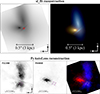 |
Fig. 3. Source plane reconstructions from SL_FIT and PYAUTOLENS. Top row: gray-scale rendering of the SL_FIT reconstructed background source morphology in the F277W band on the left and false color representation on the right obtained by combining reconstructions of the source in the F444W (red channel), F277W (green channel), and F150W (blue channel) bands. Caustic lines are overlaid in red. Bottom row: source reconstruction from PYAUTOLENS in the JWST/NIRCam F115W band (left-hand plot) and in the F444W band (middle plot) bands using identical mass models. The right-hand plot represents the superposition of the two reconstructions with F115W in blue and F444W in red. In each panel, the caustic lines are shown. North is up and east is to the left. We note that, because of the mass-sheet degeneracy (e.g., Liesenborgs & De Rijcke 2012), the scales between the two source reconstructions cannot be directly compared. |
The main parameters of the lens’ mass distribution are given in Table 1. This includes the Einstein radius θEin, magnification μ, and total mass measured within θEin. For the latter, we include three different values obtained using the three redshift solutions derived by LEPHARE, CIGALE, and EAZY on SL_FIT photometry and zlens = 2.00 ± 0.02. We stress here that magnification depends heavily on the choice of the mass distribution and in particular on its inner slope (here SIE implies γ ≡ −d log ρ/d log r = 2). The magnification that is given corresponds to a mean value derived as the flux weighted sum of the magnification experienced by the three components of the background source.
3.2. Source reconstruction and density slope using PYAUTOLENS
3.2.1. Method
Next, we performed lens modeling using the open-source software PYAUTOLENS5 (Nightingale et al. 2018b, 2021). In contrast to SL_FIT, the PYAUTOLENS analysis: (i) reconstructs the unlensed source galaxy on a Voronoi mesh which can account for irregular and asymmetric features (e.g., mergers, Nightingale & Dye 2015; Nightingale et al. 2018b); and (ii) uses information contained in the lensed source’s extended surface brightness distribution to measure more detailed properties of the lens galaxy’s mass, in this case, the power-law density slope. We give below a concise overview of the aspects of lens modeling that are the most important for this study.
Before lens modeling, preprocessing steps were performed on the data. Each band was modeled using the pixel scale closest to the native scale, that is 0.03″ for the F115W and F150W bands, and 0.06″ for the F227W and F444W bands. A 2.6″ circular mask was applied to all datasets, defining the region within which the lens analysis was performed. The emission from the feature to the south west of the Einstein ring (see Fig. 1) was removed from each image via a graphical user internal which replaces the emission with Gaussian noise. Fits including this feature were performed but the lens model indicated there was no lensing counterpart, showing that it is a foreground galaxy. We used an adaptation of the Source, Light and Mass (SLaM) pipelines described in Etherington et al. (2023) and Nightingale et al. (2023). Lens models were fitted using the nested sampling algorithm nautilus (Lange 2023). These pipelines automate the lens model fitting and are used to fit all four waveband images (F115W, F150W, F227W, and F444W) independently.
The foreground lens galaxy’s emission was modeled and subtracted using a multiple Gaussian expansion (MGE, Cappellari 2002). The MGE is implemented internally within PYAUTOLENS and performs simultaneously with the source reconstruction (He et al. in prep). The MGE decomposes the lens emission into 100 elliptical two dimensional Gaussians. Their axis-ratios, position angles and sizes vary, capturing departures from axial symmetry. The intensity of every Gaussian is solved simultaneously with the source reconstruction using a non-negative least square solver (NNLS). The MGE provides a clean deblending of the lens and source light.
The source was reconstructed using an adaptive Voronoi mesh with 2000 pixels for the higher resolution F115W and F150W bands and 1600 pixels for the F277W and F444W bands. The Voronoi pixel distribution adapts to the source morphology. This uses the natural neighbor interpolation and adaptive regularization described in Nightingale et al. (2023) but, unlike this study, it enforces positivity on source pixels by using the NNLS. The Voronoi mesh is able to reconstruct an irregular galaxy morphology, provided the mass model is accurate.
The lens galaxy mass model was used to ray-trace light from the image-plane to the unlensed source-plane, where the source reconstruction was performed. We fitted an elliptical power-law (PL) mass distribution (representing the stars and dark matter) with convergence (Suyu 2012)
where Σ(x, y) is the mass density, γ is the logarithmic slope of the mass distribution in 3D, 1 ≥ q > 0 is the projected minor to major axis ratio of the elliptical isodensity contours, and b ≥ 0 is the angular scale length of the profile. The special case γ = 2 recovers the SIE mass distribution fitted above, and q = 1 recovers the Spherical Isothermal Sphere (SIS). The profile has additional free parameters for the central coordinates (xc, yc) and position angle ϕ, measured counterclockwise from the positive x-axis. When varying the ellipticity, we actually sampled from and adjusted free parameters
because these are defined continuously in −1 < εi < 1, eliminating the periodic boundaries associated with angle ϕ and the discontinuity at q = 0. We similarly parameterized the external lensing shear as components γ1ext and γ2ext. The external shear magnitude γext and angle ϕext were recovered from these parameters by
and we included the foreground galaxy to the south west in the mass model using an SIS profile, where the center was fixed to the brightest pixel of this galaxy.
3.2.2. Results
Figure 4 shows the observed image, model, normalized residuals, and source reconstruction of fits to the COSMOS-Web ring. Across all four JWST wavelengths, the foreground lens and lensed source emission were fitted accurately, as visible in the residuals of Fig. 4. The overlaid black lines show the tangential critical curves and caustics. They are similar across each wavelength, indicating that the mass models are generally consistent. The Voronoi source reconstructions show the striking change in appearance of the source galaxy across wavelengths, where the F115W and F150W filters reveal clumpy and elongated emission from north to south and the F277W and F444W filters reconstruct an offset and compact component oriented from east to west and that is not visible at bluer wavelengths. We note that this source reconstruction is broadly consistent with that of SL_FIT that finds three Sérsic components whose spatial offset and spatial extent match the reconstructed morphology of PYAUTOLENS. We discuss in Sect. 5.4 the potential meaning of these two different components.
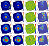 |
Fig. 4. Results of the independent PYAUTOLENS lens model fits to the F115W, F150W, F277W, and F444W bands. From left to right: observed image, lens model image, normalized residual map, and source reconstruction. North is up and east is to the left. |
The reconstructions in Fig. 4 indicate that the source’s red compact feature is not coincident with the clumpy emission reconstructed at bluer wavelengths. To confirm this, we reconstruct all wavebands using a single unified mass model derived from the highest S/N F444W image, which is shown in Fig. 3. The emission in the F444W band is clearly offset from that in the F115W band and located in a distinct region of the source-plane. Different wavelength observations are therefore detecting different components of the lensed source galaxy with the emission in the F444W band associated to the rest-frame optical (around 6700 Å) and the emission in the F115W band associated to the rest-frame UV (around 1800 Å).
The inner slope of the total mass profile inferred for the F115W, F150W, F277W and F444W filters are  ,
,  ,
,  and
and  , respectively6. The bluer F115W and F150W slope values are consistent with one another, as are the redder F277W and F444W values. However, the results at blue and red wavelengths appear inconsistent, which correlates with the bluer filters having a distinct reconstructed source morphology from the redder filters. We discuss this result in more details in Sect. 5.2.
4. Photometric redshifts and physical properties
We used three spectral energy distribution (SED) fitting codes to measure the redshift of the lens and the source. First, we started with the template-fitting code LEPHARE (Arnouts et al. 2002; Ilbert et al. 2006). We adopted a set of templates extracted from Bruzual & Charlot (2003) assuming 12 different star formation histories (SFH; exponentially declining and delayed), as described in Ilbert et al. (2015). For each SFH, we generated templates at 43 different ages (from 0.05 to 13.5 Gyr). We assumed two attenuation curves (Calzetti et al. 2000; Arnouts et al. 2013) with E(B − V) varying from 0 to 0.7. We added the emission line fluxes with a recipe described in Saito et al. (2020), following Schaerer & de Barros (2009). The normalization of the emission line fluxes was allowed to vary by a factor of two (using the same ratio for all lines) during the fitting procedure. The absorption of the intergalactic medium (IGM) was implemented following the analytical correction of Madau (1995). LEPHARE provides the redshift likelihood distribution for each object, after a marginalization over the galaxy templates and the dust attenuation. We used it as the posterior redshift probability density function (PDF), assuming a flat prior. The physical parameters were derived simultaneously.
Second, we ran EAZY (Brammer et al. 2008) to assess the robustness of the photometric redshift. We used the template set that is derived from the Flexible Stellar Population Synthesis models (FSPS; Conroy et al. 2009; Conroy & Gunn 2010, specifically QSF 12 v3), with an updated emission line template from Carnall et al. (2023). EAZY fits a non-negative linear combination of a set of basis templates to the observed flux densities for each galaxy. The latter are corrected for Milky Way extinction internally in the code and the absorption from the IGM is implemented following the prescriptions of Madau (1995). We did not apply any priors or zero-point corrections.
Finally, we also used CIGALE7 (Boquien et al. 2019), a versatile Bayesian-like analysis code modeling the X-rays to radio emission of galaxies, to derive the physical properties of the different objects, as well as assess the robustness of the photometric redshift. CIGALE includes multiple modules to model the SFH, stellar, dust, and nebular emission, as well as the active galactic nuclei (AGN) contribution to the SED. The versatility of the code is based on the ability to build and fit the different models in the context of the energy budget balance between the UV-optical emission, from the contribution of young stars, which is absorbed by dust and reemitted in IR. In this work, we used the following configuration: the sfhNlevels non-parametric module with a bursty continuity prior that was presented and tested in Ciesla et al. (2023) (see also Arango-Toro et al. 2023), the stellar population models (SSPs) of Bruzual & Charlot (2003), a Calzetti et al. (2000) attenuation law as well as the skirtor (Stalevski et al. 2016) module to model an AGN contribution. For each SED fitting code we also took into account an additional source of error that represents the uncertainties on the SED models themselves. For LEPHARE and CIGALE, we added in quadrature an error of 0.02 dex and 0.01 dex, whereas for EAZY we set a systematic floor error of 0.02 dex.
4.1. Lens
The best-fit LEPHARE SED model derived on SL_FIT photometry is shown in red in the left panel of Fig. 5. We also show in the right panel of Fig. 5 the PDF of the lens’ photometric redshift from LEPHARE (continuous line), CIGALE (dashed line), and EAZY (dotted line). The photometric redshift and physical properties derived from the different fits are given in Table 2. We get consistent results between the codes that find the lens at z ≈ 2. LEPHARE, CIGALE, and EAZY median values agree to within 0.04 which is also their typical uncertainty. Furthermore, we do not find any significant differences between the values derived from SE++ and SL_FIT photometries. Given that the morphology of the lens is not affected by the lens model and that SL_FIT and SE++ photometries are obtained from comparable Sérsic models, it is not surprising that the photometry has little impact. The lens is found to be a massive and quiescent galaxy with M⋆ > 1011 M⊙ and a specific star formation rate equal to sSFR < 10−13 yr. More precisely, LEPHARE, CIGALE, and EAZY find respectively  ,
,  , and
, and  with SE++ photometry and
  ,
,  , and
, and  with SL_FIT photometry. We note that the photometric redshift of the lens derived in this study is consistent with the value found in van Dokkum et al. (2024) and so is the total stellar mass up to a factor of two. In what follows, we use the solution from LEPHARE with SL_FIT photometry at zlens = 2.02 as a reference and we discuss how using a different solution might impact our results.
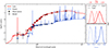 |
Fig. 5. Results from SED fitting on the foreground lens and background source and their corresponding PDFs. Left: SED fitting results from LEPHARE for the lens (red) and the source (blue) using the photometry extracted from the lens modeling with SL_FIT (see Sects. 2.3 and 3). Right: redshift PDF for the lens and the source (same colors) when using LEPHARE (continuous lines), CIGALE (dashed lines), and EAZY (dotted lines). We note that the detections in the u, g, and r bands for the source are likely contaminated by a nearby UV-bright foreground galaxy located west of the ring (see Fig. A.4.) |
Photometric redshift estimates and physical properties of the lens.
4.2. Background source
The result of the fit with LEPHARE on SL_FIT photometry is shown in blue in the left panel of Fig. 5. The PDFs from LEPHARE, CIGALE, and EAZY are shown in the right panel and the photometric redshifts and physical parameters for the various fits of the background source are given in Table 3. When using SL_FIT photometry, the source is found at  ,
,  , and
, and  with LEPHARE, CIGALE, and EAZY, respectively. However, with SE++ photometry, it is found at a lower redshift of
  ,
,  , and
, and  with LEPHARE, CIGALE, and EAZY, respectively. Thus, taking into account uncertainties, the SED fitting codes give us a range of possible photometric redshifts for the background source of 4.63 ≲ zsource ≲ 5.54.
Photometric redshift estimates and physical properties of the source. For SE++, we quote the results on CW.
We compare our photometric redshift results to that of van Dokkum et al. (2024). With our solution at zsource = 5.48 we get a χ2 = 23. On the other hand, when fitting while fixing the redshift to their solution at zsource = 2.97, we get a χ2 = 159. Besides, in the latter case the best-fit SED under-fits in bands around 1 μm and over-fit at both shorter and longer wavelengths. As in van Dokkum et al. (2024), if we restrict to HST and JWST bands, both redshifts are valid solutions, though we do get a lower χ2 = 2 with ours compared to the χ2 = 29 that we obtain when fixing to their redshift. In other terms, the detection of the source in ground-based data plays a crucial role in the determination of its photometric redshift. If we separate the contributions to the Einstein ring of Comp-1 (i.e., the background component that produces CW and CE) and Comp-2 (i.e., the blue component), we get different results. With Comp-1, we find that the solution from van Dokkum et al. (2024) at zsource = 2.97 fits slightly better the SED with a χ2 lowered from 34 (our solution) to 27 (their solution). On the opposite, our solution at zsource = 5.48 is much more robust for Comp-2 with a χ2 = 49 instead of 900 for their solution. Thus, we believe that the solution of a single background source at z ≈ 5.5 is consistent, though we cannot completely exclude the possibility that the Einstein ring might actually be the image of two galaxies superimposed along the line-of-sight, one at z ≈ 3 and another at z ≈ 5.5. Taking the density of galaxies at these two redshifts in the current version of the COSMOS-Web catalog, we get a rough estimate on the probability to observe such a superimposition of at most 0.1%.
All SED fitting solutions find that the source is quite massive with M⋆ ≳ 1010 M⊙. For a given SED fitting code, the stellar mass derived from SE++ photometry is always lower than the value derived from SL_FIT photometry. This is expected since the solution with SE++ photometry is obtained on CW only which is just a fraction of the total flux of the ring. With SL_FIT photometry, LEPHARE, CIGALE, and EAZY find a total stellar mass of  ,
,  , and
, and  , respectively. Finally, the SFR of the source is not as precisely constrained as the stellar mass with uncertainties on the order of 5 − 10 M⊙ yr. Nevertheless, all solutions find that the background source is a star-forming galaxy. Using SL_FIT photometry to estimate the SFR of the entire Einstein ring, LEPHARE and CIGALE find
  and
and  , respectively. Thus, LEPHARE and CIGALE find consistent results with SL_FIT photometry, but also when using SE++ photometry (i.e., when estimating the SFR of CW only) with
  , and
, and  , respectively. Only EAZY finds opposite trends with
  for SE++ photometry and
  for SL_FIT photometry. In other terms, EAZY finds a higher SFR in CW alone than in the entire Einstein ring. This inconsistency might be the effect of different stellar populations and dust attenuation between the red clumps and the blue part of the ring that EAZY has trouble accounting for (see Sects. 5.3 and 5.4). In what follows, we use the solution from LEPHARE with SL_FIT photometry at zsource = 5.48 as a reference and we discuss how using a different solution might impact our results.
5. Discussion
5.1. Mass budget of the central lens
We first discuss the central lens which is among the most massive galaxies at z ∼ 2 given that it lies between 0.2 and 0.6 dex above the characteristic stellar mass (Schechter 1976) of the total and passive stellar mass functions derived by Weaver et al. (2022). Its star-formation is quenched as shown by rest-frame NUV-r/r-K colors that are characteristic of evolved and passive galaxies (e.g., Arnouts et al. 2013; Moutard et al. 2020), and by its sSFR which we find to be on the order or below 10−13 yr (see Table 2). Its morphology is consistent with that of an elliptical galaxy, well described by a smooth surface brightness profile following a Sérsic law with a Sérsic index of n = 6.4 when let to vary as a free parameter. Furthermore, the lens is compact with Reff = 1.5 kpc when fitting with SOURCEXTRACTOR++ (Reff = 2.5 kpc with SL_FIT8). This size measurement is consistent with the mass-size relation of passive galaxies found at z = 2 (e.g., van der Wel et al. 2014). Given that lensing provides a constraint on the total mass of the lens (dark + baryonic; see Sect. 3) and multiwavelength observations provide constraints on its stellar mass, the combination of the two can tell us about the DM content of ETGs and how likely they could host hidden gas reservoirs. In turn, this can be used to better understand whether the quenching of the star-formation of ETGs could be the result of in situ gas stabilization processes (i.e., morphological quenching, e.g., Martig et al. 2009) or of other mechanisms (for a review on the topic, see Man & Belli 2018; Moutard et al. 2020).
First, we compare the stellar and total masses within the Einstein radius θEin = (0.78 ± 0.04)″ which is equal to 6.6 kpc at z = 2.00. Using the structural parameters of the lens derived from SL_FIT, we find that 91% of the total light is encompassed within the Einstein radius (θEin). Assuming the mass distribution follows the light distribution, it corresponds to a stellar mass within θEin of  . Given the total mass of the deflector within the Einstein radius (see Table 1), we conclude that the stellar populations contribute to (34 ± 5)% of the total mass within θEin and that there is a remaining ΔM = Mtot(<θEin) − M⋆(<θEin) = (2.46 ± 0.30) × 1011 M⊙ in the mass budget.
In order to understand if this remaining mass ΔM could be entirely attributed to the dark matter (DM) halo within the Einstein ring or not, we derived the expected DM halo mass for the lens using the stellar-to-halo mass relation (SHMR) from Shuntov et al. (2022). This SHMR was derived from a Halo Occupation Model constrained using clustering and stellar mass function measurements from the COSMOS2020 catalog (Weaver et al. 2022). This SHMR is shown in orange in the left panel of Fig. 6 and is compared to the SHRM from Behroozi et al. (2013, shown in teal) that was used in the analysis of van Dokkum et al. (2024). Using the total stellar mass of the lens derived by LEPHARE ( ), we estimate an expected DM halo mass within its virial radius of
  . We then calculated the DM mass encompassed within the Einstein radius by integrating an NFW (Navarro et al. 1997) profile9 within a cylinder of radius θEin = 6.6 kpc. We obtain
  which is consistent with the
  remaining mass not accounted for by the stellar content of the lens. Using the SHMR from Behroozi et al. (2013) instead would increase the predicted DM halo mass within the Einstein radius by roughly a factor of two. However this SHRM behaves exponentially in this mass regime, making the DM halo mass prediction so uncertain it is effectively consistent with our value derived using the SHRM from Shuntov et al. (2022) (see the dashed and dotted teal lines in the right panel of Fig. 6). Furthermore, we also get consistent results when using the stellar mass derived by CIGALE or EAZY on SL_FIT photometry.
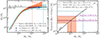 |
Fig. 6. Comparison between the DM halo mass deduced from lensing and the theoretical value obtained from stellar-to-halo mass relations (SHMRs). Left: SHMR from Shuntov et al. (2022) (in orange) and Behroozi et al. (2013) (in teal) at z ∼ 2 that we use to estimate the dark matter halo mass in which the lens resides. The solid black horizontal line marks the total stellar mass that we estimate for the lens, while the dashed vertical orange and teal lines mark the halo mass obtained from Shuntov et al. (2022) and Behroozi et al. (2013) SHMR respectively. For comparison, we also show the SHMR points from van Dokkum et al. (2024) that we derive using their total stellar mass and the Behroozi et al. (2013) SHMR as shown in the solid blue marker. The transparent blue marker shows the stellar and halo masses quoted in van Dokkum et al. (2024). Right: relation between projected mass within the Einstein radius and total halo mass. The orange dashed line and shaded regions show the results from Shuntov et al. (2022) SHMR, while the teal thick and thin dashed lines show results and the lower limit on the uncertainty from Behroozi et al. (2013) SHMR. The purple thick line shows the dark matter mass derived as Mtot(< θEin)−M⋆(< θEin), while the thin one shows the total mass derived from the SL_FIT modeling. For comparison, we also show the results quoted in van Dokkum et al. (2024) in a dashed-dotted blue line. |
We note that both our stellar mass derived from SED fitting and our expected DM halo mass derived from the SHRM are consistent with the values from van Dokkum et al. (2024). However, in their analysis, the sum of the two components is not sufficient to account for the total mass derived from lensing whereas, in our case, it is sufficient. This is because our total mass estimates within the Einstein radius are different. They find  whereas we find Mtot(<θEin) = (3.66 ± 0.36 ×) × 1011 M⊙ instead. Since our Einstein radius and lens photometric redshifts agree, the main reason for this large difference is the fact that they find the background source at
  whereas we find it at zsource = 5.48 ± 0.06.
Given that the solution at z < 3 is disfavored by our SED fitting results when taking into account ground-based observations, we conclude that the mass budget of the lens is consistent with the presence of a DM halo mass of total mass  . Thus, we do not need any gas mass contribution to explain our results. By taking the extreme 1σ uncertainties on our mass estimates, we find an upper limit on the gas mass in the lens of Mgas(<θEin) = 0.8 × 10¹¹ M⊙, consistent with recent estimates of the gas mass fraction in ETGs at z ∼ 2 of 5 − 10% of the stellar mass (e.g., Magdis et al. 2021; Caliendo et al. 2021; Whitaker et al. 2021). Given the predicted low gas mass, morphological quenching is unlikely. On the other hand, since the halo is ten times more massive than the critical mass of 1012 M⊙, hot gas quenching (e.g., Cattaneo et al. 2006; Gabor & Davé 2015) could be a potential mechanism that led to the formation of this ETG.
5.2. Total mass density profile of the lens
Measurements of the inner slope of the total mass density profile of ETGs inform us of how they evolve, for example about the contribution of minor and major mergers and the role of processes such as black hole feedback (e.g., Wang et al. 2019, 2020). The slope of over 50 ETG strong lenses have been measured, with different correlations with redshift being claimed (e.g., Bolton et al. 2012; Sonnenfeld et al. 2013; Etherington et al. 2023). Existing statistically significant lens samples extend to redshifts of zlens ∼ 0.8. The COSMOS-Web ring offers a first insight into the density slope of ETGs at z ∼ 2. Figure 7 compares the COSMOS-Web ring’s slope measurement to 44 values inferred in Etherington et al. (2023), who used the same technique as this study. The measurement of Wong et al. (2014) is also shown, which was the previous highest redshift slope measurement in a lens. All of our four measured γ values for the COSMOS-Web ring are steeper than isothermal profiles (γ = 2), suggesting that higher redshift lenses may not have shallower density profiles than the local Universe average value around γ = 2.06 (Koopmans et al. 2009). However, with just a single lens and the large range of plausible γ values measured, we cannot yet generalize our results to the broader population of ETGs.
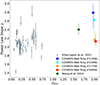 |
Fig. 7. Inner slope γ of the total mass profile of the lens as a function of redshift for 44 strong lenses from Etherington et al. (2023) (blue points) and the high redshift lens studied by Wong et al. (2014) (green point). Independent values for the COSMOS-Web ring are shown for F115W (blue), F150W (cyan), F277W (orange), and F444W (red). |
Nevertheless, this study shows that lenses found via JWST surveys similar to COSMOS-Web will enable slope measurements extending to much higher zlens values than previously. We have also demonstrated that slope measurements is possible from the same JWST imaging data required to find the lens in the first place. Therefore, once the expected ∼50 to 100 lenses contained within the COSMOS-Web data are found (Casey et al. 2023; Holloway et al. 2023), this measurement will be possible on large lens samples.
The disparity between γ measurements at bluer (F115W, F150W) and redder (F277W, F444W) wavelengths is noteworthy. The slope inferred via lens modeling depends on where the lensed source probes the mass distribution of the lens. In the bluer filters the source is brightest to the north and south of the lens, whereas in redder filters it is to the east and west. These different measurements might therefore indicate that the projected density of the lens varies azimuthally. This could be consistent with results from Nightingale et al. (2019) that showed that such effects could be possible because lenses may have distinct internal stellar structures. Ultimately, this would imply the underlying mass distribution of the lens is more complex than a power-law, as has been argued by other studies (Schneider & Sluse 2014; Etherington et al. 2023). However, instrumental effects might also cause such effects given that different pixel scales are used between blue and red JWST wavelengths and that the PSF shape and size significantly varies between those bands. Ideally, one should combine these lensing observations with stellar kinematics follow-ups to better probe the inner structure of the total mass distribution of the lens.
5.3. Multiple galaxies in the source
When doing a source reconstruction, we find that the source has a highly irregular shape, as illustrated in Fig. 3. Given their differences in methodology, it is interesting to note that both PYAUTOLENS and SL_FIT find similar results. The source seems to be made of at least two distinct components. The first one (Comp-1) is modeled as a compact galaxy oriented from east to west. It is mostly visible in the F444W band and it is the main contributor to CW and CE in the Einstein ring. Furthermore, its stellar mass derived on SL_FIT photometry is M⋆ ≈ 1 − 3 × 10¹⁰ M⊙ (taking into account the flux in both CW and CE). The second component (Comp-2) is more extended by roughly a factor of two with respect to Comp-1, oriented from north to south, and is offset to the east by about 0.15″ (roughly 1 kpc; see Fig. 3). Comp-2 appears much less massive than Comp-1 with M⋆ ≈ 109 M⊙. When summed up, the stellar mass of Comp-1 and Comp-2 is consistent within the uncertainties with the stellar mass derived on the photometry of the whole ring from SL_FIT (see Table 3). As discussed in Sect. 4.2, based on our fits with and without ground-based observations, a solution at zsource > 5 is more likely. In particular, this solution appears very robust for Comp-2 compared to that of van Dokkum et al. (2024) at zsource = 2.97. However, we cannot easily discard the latter for Comp-1 given that its SED fits slightly better than the best-fit solution found at zsource = 5.48 (χ2 = 27 instead of 34). A possibility could therefore be that the Einstein ring is actually the image produced by the superimposition along the line-of-sight of two galaxies at different redshifts. One way to determine whether that is the case or not is with follow-up observations using slit or integral field spectroscopy (e.g., X-shooter or NIRSpec IFU).
Assuming the source is located at a single redshift, then a second possibility is that the source is actually two galaxies in a merging process. The complex reconstructed morphology, the spatial offset between Comp-1 and Comp-2 by about 1 kpc, and the differences in stellar mass, SFR, and color could be indications that there are two galaxies, potentially in interaction. If so, then the mass ratio between the two galaxies would be in the range of 1:15–1:75 given the uncertainties on the stellar masses of the two components which would correspond to a minor merger (e.g., Ventou et al. 2017, 2019). We note that this scenario would also be consistent with the fact that the component with the lowest stellar mass is the most extended one, for instance because of tidal stripping.
5.4. A partially dust-obscured star-forming galaxy
The source could also be a dust-obscured galaxy whose dust is inhomogeneously located throughout the galaxy. In particular, this could explain why the clumps CW and CE appear much redder than the rest of the ring as well as the highly irregular morphology, as suggested by both observations (e.g., Dye et al. 2015; Massardi et al. 2018) and simulations (e.g., Cochrane et al. 2019). To check for the presence of dust, we have used FIR detections from Jin et al. (in prep.) as discussed in the last paragraph of Sect. 2.1. We do not get any detection in MIPS and PACS bands (S/N < 1) and tentative detections with S/N ≈ 1.5 in the three SPIRE bands when taking into account the confusion noise.
However, we do measure a flux of (4.9 ± 1.1)Mil Jky in SCUBA-2 (S/N ≈ 4.3). Its peak is not centered on the ring but offset to the south west, though the coarser resolution of SCUBA-2 (beam ∼15″) make it difficult to determine its exact location (see Fig. A.1). Because the lens is a passive elliptical galaxy, its FIR emission is expected to be low and not detectable in SCUBA-2, as indicated by the stacked FIR SEDs of z ∼ 2 quiescent samples (e.g., Magdis et al. 2021). Besides, the mass analysis of the lens presented in Sect. 5.1 is also consistent with little to no gas and therefore dust in the lens. In addition, CW and CE are the reddest objects detected in NIRCam within the SCUBA-2 beam, which is in favor of the ring being the origin of the dust emission. Still, the nearby companion at z ≈ 2 could also contribute.
Within the Einstein ring, the two reddest components are CW and CE which could suggest that, if the background source is dusty, it is inhomogeneously distributed. This is supported by the fact that the best-fit SED model from LEPHARE finds an attenuation of E(B − V) = 0.7 for Comp-1 (i.e., for the clumps in the ring) but only E(B − V) = 0.1 for Comp-2 which corresponds to the blue component of the ring. Another option is given by the fact that Hα falls within the F444W band at zsource ∼ 5.5 in which case the difference in color between the clumps and the rest of the ring would be produced by star-formation. However, when comparing the SEDs of Comp-1 and Comp-2 we find that this explanation is unlikely since LEPHARE was allowed to boost the emission line fluxes by up to a factor of two and never converged to such a solution. Therefore, the more likely scenario is that the background source is a dusty star-forming galaxy at z > 5 with an inhomogeneous distribution of dust.
Finally, we can also compare our stellar mass and SFR estimates to the Main Sequence (MS) of Khusanova et al. (2021). Their MS was obtained from the ALPINE-ALMA [C II] survey (Béthermin et al. 2020; Le Fèvre et al. 2020; Faisst et al. 2020) by estimating with ALMA the fraction of dust-obscured SFR in galaxies at z ∼ 4 − 5 from their rest-frame FIR continuum. Taking their Fig. 10, they find a SFR ≈ 30 M⊙ yr for M⋆ = 1010 M⊙ and SFR ≈ 100 M⊙ yr for M⋆ = 5 × 10¹⁰ M⊙. Thus, the source falls within their MS. If the source is instead at zsource ≈ 4.5 and with M⋆ > 1010 M⊙, then it would rather lie just below their best-fit MS with a difference ΔSFR ≳ 100 M⊙ yr. We reach similar conclusions when comparing our results to the best-fit MS at 1 Gyr from Popesso et al. (2023).
6. Conclusions
We have presented in this paper an in-depth analysis of the COSMOS-Web ring. We serendipitously discovered it during the data reduction of the COSMOS-Web survey in April 2023. Similarly, it has been independently discovered by another team and presented in van Dokkum et al. (2024). Our separate analysis leads to the following findings. The system comprises a central lens and a full Einstein ring with two red clumps noted CW and CE and mostly detected in the F444W band. A nearby companion is also located to the south west. It is found at z ≈ 2 and is therefore likely associated with the lens. Thanks to the wealth of multiwavelength observations in COSMOS-Web, we combined our JWST data with ground- and space-based observations from the visible to the FIR domain. Besides JWST, the COSMOS-Web ring is also detected in HST/ACS F814W, UltraVISTA, and HSC-i bands. However, these previous observations lacked sufficient resolution and S/N to identify the lens. Thus, the COSMOS-Web ring was effectively unnoticed by previous strong lens catalogs prior to the advent of JWST observations in COSMOS-Web.
By combining more than 25 bands from the u-band to the NIR and using robust model fitting techniques, we have extracted the photometry of both the lens and the source. This allowed us to derive the photometric redshifts and the physical properties of the lens and the source with three different SED fitting codes (CIGALE, LEPHARE, and EAZY). For the lens, we find consistent results that make it a red, compact (Sérsic index n = 6.4), massive ( ), and quiescent (sSFR ≲ 10−13 M⊙ yr) ETG at zlens = 2.02 ± 0.02. Given its size (Reff = 1.5 kpc), it falls on the typical mass-size relation found for ETGs at the same redshift. For the source, our results also consistently show that it is a massive (
 ) and star-forming galaxy (
 ) at zsource ≈ 5.48 ± 0.06. These values are consistent with those from van Dokkum et al. (2024), except for the redshift of the background source that they find at zsource ≈ 2.93 instead. Overall, we find no evidence for a solution at zsource < 3, except when fitting the red component of the ring alone, in which case both zsource ≈ 3 and zsource ≈ 5.5 appear as valid solutions.
In addition, we have also carried out two different and complementary lens modelings on JWST images. The first one is SL_FIT and uses a parametric approach to model the morphology of the source whereas the second one is PYAUTOLENS and uses a pixel-grid reconstruction technique. This has allowed us to (i) constrain the mass budget of the lens by measuring its total mass within the Einstein radius, (ii) provide a first constraint of the inner slope of the total mass density profile of an ETG at z ∼ 2, and (iii) reconstruct the complex morphology of the source. Both techniques provide fairly consistent results where the reconstructed morphology of the source is complex and highly waveband-dependent with at least two distinct components offset from each other. The best-fit mass profile slope γ from PYAUTOLENS systematically goes down from  in the F115W band to
  in the F444W band. While a single lens is not sufficient to constrain the evolution of the slope of the total mass profiles of ETGs since z ∼ 2, the COSMOS-Web ring is always found to have a value above the average γ = 2.06 found in the local Universe.
We analyzed the contribution of the baryonic and dark matter components to the total mass budget of the lens by comparing:
-
(i)
The stellar mass measured from SED fitting,
-
(ii)
The halo mass expected from SHMR relations, and
-
(iii)
The total mass inferred from lensing.
This mass budget is established within the Einstein radius. Our results consistently show that the total mass budget can be fully accounted for by the measured stellar and dark matter masses. These conclusions are robust and hold for any set of stellar mass estimates and SHMR that we tested. We conclude that the ETG is likely hosted by a DM halo mass of  . We also conclude that we do not need any gas mass contribution with an upper-limit of Mgas(<θEin) = 0.8 × 10¹¹ M⊙. Therefore, in contrast to the findings in van Dokkum et al. (2024) we report no missing mass and no need to change the IMF or the DM halo profile to interpret it. We find that the main reason behind our two opposite conclusions is that van Dokkum et al. (2024) estimate a total mass a factor of two higher than ours because of their lower redshift for the source.
The morphology of the source reconstructed from the lens modeling is fairly consistent between the two methods we adopted. In both cases, at least two different components are necessary to account for the complex ring shape. The first one is relatively compact, accounts for the bulk of the stellar mass in the ring, and is the main contributor to CW and CE. The second component is about twice as extended as the first component, is offset to the west by roughly 1 kpc and mostly emits in the F115W and F150W bands. The source is likely a single galaxy at zsource ≈ 5.5 but, given the complex reconstructed morphology and that the solution at zsource = 2.93 is also plausible for the red component, we cannot discard the possibility that the source is the superimposition along the line-of-sight of two galaxies at z ≈ 3 and 5.5. If so, we estimate an upper limit on the probability to happen of 0.1%. Furthermore, without spatially resolved spectroscopy (e.g., NIRSpec IFU or ALMA), we also cannot discard the possibility that the source is actually a merger. If so, then the mass ratio of the two components would suggest that the source is a minor merger, with potentially one of the two galaxies being tidally stripped.
Finally, by cross-correlating the position of the COSMOS-Web ring with the Super-deblended catalog of Jin et al. (in prep.), we find a nearby detection at S/N = 4.3 in SCUBA-2 and tentative detections in Herschel/SPIRE bands. Given the position of the SCUBA-2 beam, the passive nature of the lens, and the large dust attenuation found by LEPHARE in CW and CE, we estimate that the FIR detections likely originate from the clumps. This would make the background source a dusty star-forming galaxy with a potentially heterogeneous dust distribution. This system offers exciting opportunities for studying star formation in a resolved galaxy during the first billion years of the Universe.
The median seeing is around 0.9″ in the u-band (Sawicki et al. 2019) and 0.6″ in the i-band (Aihara et al. 2022).
As discussed in Sect. 6.8 of Nightingale et al. (2018a), the uncertainties are computed as the 3σ bounds on the marginalized posterior distribution.
While a factor of about 1.7 on the effective radius may appear significant, we note that this parameter is found to be degenerate with the Sérsic index. As illustrated in Fig. 2 both models fit equally well the lens.
Where we assume a Dutton & Macciò (2014) mass-concentration relationship and not take into consideration the scatter in this relationship in our discussion.
Acknowledgments
We thank the referee for providing useful and constructive comments on the submitted version of this paper. This research is also partly supported by the Centre National d’Etudes Spatiales (CNES). We acknowledge the funding of the French Agence Nationale de la Recherche for the project iMAGE (grant ANR-22-CE31-0007). We warmly acknowledge the contributions of the entire COSMOS collaboration consisting of more than 100 scientists. The HST-COSMOS program was supported through NASA grant HST-GO-09822. More information on the COSMOS survey is available at https://cosmos.astro.caltech.edu. This work was made possible by utilizing the CANDIDE cluster at the Institut d’Astrophysique de Paris, which was funded through grants from the PNCG, CNES, DIM-ACAV, and the Cosmic Dawn Center and maintained by S. Rouberol. JWN is supported by the UK Space Agency, through grant ST/N001494/1. JR was supported by JPL, which is operated by Caltech under a contract for NASA. GEM acknowledges the Villum Fonden research grant 13160 “Gas to stars, stars to dust: tracing star formation across cosmic time”, grant 37440, “The Hidden Cosmos”. The Cosmic Dawn Center (DAWN) is funded by the Danish National Research Foundation under the grant DNRF140. SJ is supported by the European Union’s Horizon Europe research and innovation program under the Marie Skłodowska-Curie grant agreement No. 101060888. JN, GM and RM are supported by STFC via grant ST/X001075/1, and the UK Space Agency via grant ST/X001997/1. AA is supported by the European Research Council via grant DMIDAS (GA 786910). This work used both the Cambridge Service for Data Driven Discovery (CSD3) and the DiRAC Data-Centric system, which are operated by the University of Cambridge and Durham University on behalf of the STFC DiRAC HPC Facility (https://www.dirac.ac.uk). These were funded by BIS capital grant ST/K00042X/1, STFC capital grants ST/P002307/1, ST/R002452/1, ST/H008519/1, ST/K00087X/1, STFC Operations grants ST/K003267/1, ST/K003267/1, and Durham University. DiRAC is part of the UK National E-Infrastructure.
References
- Aihara, H., Arimoto, N., Armstrong, R., et al. 2018, PASJ, 70, S4 [NASA ADS] [Google Scholar]
- Aihara, H., AlSayyad, Y., Ando, M., et al. 2022, PASJ, 74, 247 [NASA ADS] [CrossRef] [Google Scholar]
- Arango-Toro, R. C., Ciesla, L., Ilbert, O., et al. 2023, A&A, 675, A126 [NASA ADS] [CrossRef] [EDP Sciences] [Google Scholar]
- Arnouts, S., Moscardini, L., Vanzella, E., et al. 2002, MNRAS, 329, 355 [Google Scholar]
- Arnouts, S., Le Floc’h, E., Chevallard, J., et al. 2013, A&A, 558, A67 [NASA ADS] [CrossRef] [EDP Sciences] [Google Scholar]
- Atek, H., Chemerynska, I., Wang, B., et al. 2023, MNRAS, 524, 5486 [NASA ADS] [CrossRef] [Google Scholar]
- Auger, M. W., Treu, T., Bolton, A. S., et al. 2010, ApJ, 724, 511 [NASA ADS] [CrossRef] [Google Scholar]
- Behroozi, P. S., Wechsler, R. H., & Conroy, C. 2013, ApJ, 770, 57 [NASA ADS] [CrossRef] [Google Scholar]
- Bergamini, P., Acebron, A., Grillo, C., et al. 2023, ApJ, 952, 84 [NASA ADS] [CrossRef] [Google Scholar]
- Bertin, E. 2011, in Astronomical Data Analysis Software and Systems XX, eds. I. N. Evans, A. Accomazzi, D. J. Mink, & A. H. Rots, ASP Conf. Ser., 442, 435 [Google Scholar]
- Bertin, E., Schefer, M., Apostolakos, N., et al. 2020, in Astronomical Data Analysis Software and Systems XXIX, eds. R. Pizzo, E. R. Deul, J. D. Mol, J. de Plaa, & H. Verkouter, ASP Conf. Ser., 527, 461 [NASA ADS] [Google Scholar]
- Béthermin, M., Fudamoto, Y., Ginolfi, M., et al. 2020, A&A, 643, A2 [Google Scholar]
- Bezanson, R., Labbe, I., Whitaker, K. E., et al. 2022, ApJ, submitted, [arXiv:2212.04026] [Google Scholar]
- Bolamperti, A., Grillo, C., Cañameras, R., Suyu, S. H., & Christensen, L. 2023, A&A, 671, A60 [NASA ADS] [CrossRef] [EDP Sciences] [Google Scholar]
- Bolton, A. S., Brownstein, J. R., Kochanek, C. S., et al. 2012, ApJ, 757, 82 [NASA ADS] [CrossRef] [Google Scholar]
- Boquien, M., Burgarella, D., Roehlly, Y., et al. 2019, A&A, 622, A103 [NASA ADS] [CrossRef] [EDP Sciences] [Google Scholar]
- Brammer, G. B., van Dokkum, P. G., & Coppi, P. 2008, ApJ, 686, 1503 [Google Scholar]
- Brault, F., & Gavazzi, R. 2015, A&A, 577, A85 [NASA ADS] [CrossRef] [EDP Sciences] [Google Scholar]
- Browne, I. W. A., Wilkinson, P. N., Jackson, N. J. F., et al. 2003, MNRAS, 341, 13 [NASA ADS] [CrossRef] [Google Scholar]
- Bruzual, G., & Charlot, S. 2003, MNRAS, 344, 1000 [NASA ADS] [CrossRef] [Google Scholar]
- Bushouse, H., Eisenhamer, J., Dencheva, N., et al. 2022, https://doi.org/10.5281/zenodo.7325378 [Google Scholar]
- Caliendo, J. N., Whitaker, K. E., Akhshik, M., et al. 2021, ApJ, 910, L7 [NASA ADS] [CrossRef] [Google Scholar]
- Calzetti, D., Armus, L., Bohlin, R. C., et al. 2000, ApJ, 533, 682 [NASA ADS] [CrossRef] [Google Scholar]
- Campusano, L. E., Pelló, R., Kneib, J. P., et al. 2001, A&A, 378, 394 [NASA ADS] [CrossRef] [EDP Sciences] [Google Scholar]
- Cañameras, R., Nesvadba, N. P. H., Kneissl, R., et al. 2017, A&A, 600, L3 [Google Scholar]
- Cañameras, R., Schuldt, S., Suyu, S. H., et al. 2020, A&A, 644, A163 [Google Scholar]
- Cañameras, R., Schuldt, S., Shu, Y., et al. 2023, A&A, submitted, [arXiv:2306.03136] [Google Scholar]
- Cappellari, M. 2002, MNRAS, 333, 400 [NASA ADS] [CrossRef] [Google Scholar]
- Carnall, A. C., McLeod, D. J., McLure, R. J., et al. 2023, MNRAS, 520, 3974 [NASA ADS] [CrossRef] [Google Scholar]
- Casey, C. M., Kartaltepe, J. S., Drakos, N. E., et al. 2023, ApJ, 954, 31 [NASA ADS] [CrossRef] [Google Scholar]
- Cattaneo, A., Dekel, A., Devriendt, J., Guiderdoni, B., & Blaizot, J. 2006, MNRAS, 370, 1651 [NASA ADS] [CrossRef] [Google Scholar]
- Chabrier, G. 2003, PASP, 115, 763 [Google Scholar]
- Ciesla, L., Béthermin, M., Daddi, E., et al. 2020, A&A, 635, A27 [NASA ADS] [CrossRef] [EDP Sciences] [Google Scholar]
- Ciesla, L., Gómez-Guijarro, C., Buat, V., et al. 2023, A&A, 672, A191 [NASA ADS] [CrossRef] [EDP Sciences] [Google Scholar]
- Claeyssens, A., Richard, J., Blaizot, J., et al. 2022, A&A, 666, A78 [NASA ADS] [CrossRef] [EDP Sciences] [Google Scholar]
- Claeyssens, A., Adamo, A., Richard, J., et al. 2023, MNRAS, 520, 2180 [NASA ADS] [CrossRef] [Google Scholar]
- Cochrane, R. K., Hayward, C. C., Anglés-Alcázar, D., et al. 2019, MNRAS, 488, 1779 [NASA ADS] [CrossRef] [Google Scholar]
- Collett, T. E. 2015, ApJ, 811, 20 [NASA ADS] [CrossRef] [Google Scholar]
- Conroy, C., & Gunn, J. E. 2010, ApJ, 712, 833 [Google Scholar]
- Conroy, C., Gunn, J. E., & White, M. 2009, ApJ, 699, 486 [Google Scholar]
- Diehl, H. T., Buckley-Geer, E. J., Lindgren, K. A., et al. 2017, ApJS, 232, 15 [NASA ADS] [CrossRef] [Google Scholar]
- Dunlop, J. S. 2016, UltraVISTA - Ultra Deep Survey with VISTA (European Southern Observatory (ESO)) [Google Scholar]
- Dutton, A. A., & Macciò, A. V. 2014, MNRAS, 441, 3359 [Google Scholar]
- Dye, S., Negrello, M., Hopwood, R., et al. 2014, MNRAS, 440, 2013 [NASA ADS] [CrossRef] [Google Scholar]
- Dye, S., Furlanetto, C., Swinbank, A. M., et al. 2015, MNRAS, 452, 2258 [NASA ADS] [CrossRef] [Google Scholar]
- Etherington, A., Nightingale, J. W., Massey, R., et al. 2023, MNRAS, 521, 6005 [CrossRef] [Google Scholar]
- Faisst, A. L., Schaerer, D., Lemaux, B. C., et al. 2020, ApJS, 247, 61 [NASA ADS] [CrossRef] [Google Scholar]
- Faure, C., Kneib, J.-P., Covone, G., et al. 2008a, ApJS, 178, 382 [NASA ADS] [CrossRef] [Google Scholar]
- Faure, C., Kneib, J.-P., Covone, G., et al. 2008b, ApJS, 176, 19 [NASA ADS] [CrossRef] [Google Scholar]
- Gabor, J. M., & Davé, R. 2015, MNRAS, 447, 374 [NASA ADS] [CrossRef] [Google Scholar]
- Garvin, E. O., Kruk, S., Cornen, C., et al. 2022, A&A, 667, A141 [NASA ADS] [CrossRef] [EDP Sciences] [Google Scholar]
- Gavazzi, R., & Soucail, G. 2007, A&A, 462, 459 [NASA ADS] [CrossRef] [EDP Sciences] [Google Scholar]
- Gavazzi, R., Treu, T., Koopmans, L. V. E., et al. 2008, ApJ, 677, 1046 [NASA ADS] [CrossRef] [Google Scholar]
- Gavazzi, R., Cooray, A., Conley, A., et al. 2011, ApJ, 738, 125 [NASA ADS] [CrossRef] [Google Scholar]
- Gavazzi, R., Treu, T., Marshall, P. J., Brault, F., & Ruff, A. 2012, ApJ, 761, 170 [Google Scholar]
- Gavazzi, R., Marshall, P. J., Treu, T., & Sonnenfeld, A. 2014, ApJ, 785, 144 [Google Scholar]
- Graham, A., Lauer, T. R., Colless, M., & Postman, M. 1996, ApJ, 465, 534 [NASA ADS] [CrossRef] [Google Scholar]
- Hezaveh, Y. D., & Holder, G. P. 2011, ApJ, 734, 52 [NASA ADS] [CrossRef] [Google Scholar]
- Hezaveh, Y. D., Marrone, D. P., Fassnacht, C. D., et al. 2013, ApJ, 767, 132 [NASA ADS] [CrossRef] [Google Scholar]
- Holloway, P., Verma, A., Marshall, P. J., More, A., & Tecza, M. 2023, MNRAS, 525, 2341 [CrossRef] [Google Scholar]
- Hsiao, T. Y.-Y., Abdurro’uf, Coe, D., et al. 2023, ApJ, submitted, [arXiv:2305.03042] [Google Scholar]
- Huchra, J., Gorenstein, M., Kent, S., et al. 1985, AJ, 90, 691 [NASA ADS] [CrossRef] [Google Scholar]
- Ilbert, O., Arnouts, S., McCracken, H. J., et al. 2006, A&A, 457, 841 [NASA ADS] [CrossRef] [EDP Sciences] [Google Scholar]
- Ilbert, O., Arnouts, S., Le Floc’h, E., et al. 2015, A&A, 579, A2 [NASA ADS] [CrossRef] [EDP Sciences] [Google Scholar]
- Jackson, N. 2008, MNRAS, 389, 1311 [NASA ADS] [CrossRef] [Google Scholar]
- Jauncey, D. L., Reynolds, J. E., Tzioumis, A. K., et al. 1991, Nature, 352, 132 [Google Scholar]
- Jauzac, M., Richard, J., Jullo, E., et al. 2015, MNRAS, 452, 1437 [Google Scholar]
- Jin, S., Daddi, E., Liu, D., et al. 2018, ApJ, 864, 56 [Google Scholar]
- Johnson, T. L., Rigby, J. R., Sharon, K., et al. 2017a, ApJ, 843, L21 [Google Scholar]
- Johnson, T. L., Sharon, K., Gladders, M. D., et al. 2017b, ApJ, 843, 78 [NASA ADS] [CrossRef] [Google Scholar]
- Jones, T. A., Swinbank, A. M., Ellis, R. S., Richard, J., & Stark, D. P. 2010, MNRAS, 404, 1247 [NASA ADS] [Google Scholar]
- Khusanova, Y., Bethermin, M., Le Fèvre, O., et al. 2021, A&A, 649, A152 [NASA ADS] [CrossRef] [EDP Sciences] [Google Scholar]
- Kneib, J. P., Ellis, R. S., Smail, I., Couch, W. J., & Sharples, R. M. 1996, ApJ, 471, 643 [Google Scholar]
- Koekemoer, A. M., Aussel, H., Calzetti, D., et al. 2007, ApJS, 172, 196 [Google Scholar]
- Koopmans, L. V., Bolton, A., Treu, T., et al. 2009, ApJ, 703 [Google Scholar]
- Kümmel, M., Bertin, E., Schefer, M., et al. 2020, in Astronomical Data Analysis Software and Systems XXIX, eds. R. Pizzo, E. R. Deul, J. D. Mol, J. de Plaa, & H. Verkouter, ASP Conf. Ser., 527, 29 [Google Scholar]
- Lange, J. U. 2023, MNRAS, 525, 3181 [NASA ADS] [CrossRef] [Google Scholar]
- Le Fèvre, O., Béthermin, M., Faisst, A., et al. 2020, A&A, 643, A1 [Google Scholar]
- Liesenborgs, J., & De Rijcke, S. 2012, MNRAS, 425, 1772 [CrossRef] [Google Scholar]
- Liu, D., Daddi, E., Dickinson, M., et al. 2018, ApJ, 853, 172 [Google Scholar]
- Livermore, R. C., Jones, T., Richard, J., et al. 2012, MNRAS, 427, 688 [NASA ADS] [CrossRef] [Google Scholar]
- Livermore, R. C., Jones, T. A., Richard, J., et al. 2015, MNRAS, 450, 1812 [Google Scholar]
- Lynds, R., & Petrosian, V. 1986, BAAS, 18, 1014 [NASA ADS] [Google Scholar]
- Madau, P. 1995, ApJ, 441, 18 [NASA ADS] [CrossRef] [Google Scholar]
- Magdis, G. E., Gobat, R., Valentino, F., et al. 2021, A&A, 647, A33 [NASA ADS] [CrossRef] [EDP Sciences] [Google Scholar]
- Man, A., & Belli, S. 2018, Nat. Astron., 2, 695 [NASA ADS] [CrossRef] [Google Scholar]
- Martig, M., Bournaud, F., Teyssier, R., & Dekel, A. 2009, ApJ, 707, 250 [Google Scholar]
- Massardi, M., Enia, A. F. M., Negrello, M., et al. 2018, A&A, 610, A53 [NASA ADS] [CrossRef] [EDP Sciences] [Google Scholar]
- Massey, R., Harvey, D., Liesenborgs, J., et al. 2018, MNRAS, 477, 669 [NASA ADS] [CrossRef] [Google Scholar]
- McCracken, H. J., Milvang-Jensen, B., Dunlop, J., et al. 2012, A&A, 544, A156 [NASA ADS] [CrossRef] [EDP Sciences] [Google Scholar]
- Meštrić, U., Vanzella, E., Zanella, A., et al. 2022, MNRAS, 516, 3532 [CrossRef] [Google Scholar]
- Moutard, T., Malavasi, N., Sawicki, M., Arnouts, S., & Tripathi, S. 2020, MNRAS, 495, 4237 [CrossRef] [Google Scholar]
- Myers, S. T., Jackson, N. J., Browne, I. W. A., et al. 2003, MNRAS, 341, 1 [Google Scholar]
- Navarro, J. F., Frenk, C. S., & White, S. D. M. 1997, ApJ, 490, 493 [Google Scholar]
- Negrello, M., Hopwood, R., De Zotti, G., et al. 2010, Science, 330, 800 [NASA ADS] [CrossRef] [Google Scholar]
- Negrello, M., Amber, S., Amvrosiadis, A., et al. 2017, MNRAS, 465, 3558 [NASA ADS] [CrossRef] [Google Scholar]
- Nguyen, H. T., Schulz, B., Levenson, L., et al. 2010, A&A, 518, L5 [NASA ADS] [CrossRef] [EDP Sciences] [Google Scholar]
- Nightingale, J. W., & Dye, S. 2015, MNRAS, 452, 2940 [Google Scholar]
- Nightingale, J. W., Dye, S., & Massey, R. J. 2018a, MNRAS, 478, 4738 [Google Scholar]
- Nightingale, J. W., Hayes, R., Dye, S., Massey, R. J., & Frenk, C. S. 2018b, PyAutoLens: Strong lens modeling, Astrophysics Source Code Library [record ascl:1807.003] [Google Scholar]
- Nightingale, J. W., Massey, R. J., Harvey, D. R., et al. 2019, MNRAS, 489, 2049 [NASA ADS] [Google Scholar]
- Nightingale, J., Hayes, R., Kelly, A., et al. 2021, J. Open Source Software, 6, 2825 [NASA ADS] [CrossRef] [Google Scholar]
- Nightingale, J. W., Smith, R. J., He, Q., et al. 2023, MNRAS, 521, 3298 [NASA ADS] [CrossRef] [Google Scholar]
- O’Donnell, J. H., Wilkinson, R. D., Diehl, H. T., et al. 2022, ApJ, 259, 27 [Google Scholar]
- Oguri, M., Rusu, C. E., & Falco, E. E. 2014, MNRAS, 439, 2494 [Google Scholar]
- Oke, J. B. 1974, ApJS, 27, 21 [Google Scholar]
- Petrillo, C. E., Tortora, C., Chatterjee, S., et al. 2017, MNRAS, 472, 1129 [Google Scholar]
- Popesso, P., Concas, A., Cresci, G., et al. 2023, MNRAS, 519, 1526 [Google Scholar]
- Pourrahmani, M., Nayyeri, H., & Cooray, A. 2018, ApJ, 856, 68 [NASA ADS] [CrossRef] [Google Scholar]
- Richard, J., Claeyssens, A., Lagattuta, D., et al. 2021, A&A, 646, A83 [EDP Sciences] [Google Scholar]
- Rojas, K., Savary, E., Clément, B., et al. 2022, A&A, 668, A73 [NASA ADS] [CrossRef] [EDP Sciences] [Google Scholar]
- Saito, S., de la Torre, S., Ilbert, O., et al. 2020, MNRAS, 494, 199 [NASA ADS] [CrossRef] [Google Scholar]
- Savary, E., Rojas, K., Maus, M., et al. 2022, A&A, 666, A1 [NASA ADS] [CrossRef] [EDP Sciences] [Google Scholar]
- Sawicki, M., Arnouts, S., Huang, J., et al. 2019, MNRAS, 489, 5202 [NASA ADS] [Google Scholar]
- Schechter, P. 1976, ApJ, 203, 297 [Google Scholar]
- Schaerer, D., & de Barros, S. 2009, A&A, 502, 423 [NASA ADS] [CrossRef] [EDP Sciences] [Google Scholar]
- Schneider, P., & Sluse, D. 2014, A&A, 564, A104 [NASA ADS] [CrossRef] [EDP Sciences] [Google Scholar]
- Shuntov, M., McCracken, H. J., Gavazzi, R., et al. 2022, A&A, 664, A61 [NASA ADS] [CrossRef] [EDP Sciences] [Google Scholar]
- Sonnenfeld, A., Treu, T., Gavazzi, R., et al. 2013, ApJ, 777, 98 [Google Scholar]
- Sonnenfeld, A., Chan, J. H. H., Shu, Y., et al. 2018, PASJ, 70, S29 [Google Scholar]
- Sonnenfeld, A., Verma, A., More, A., et al. 2020, A&A, 642, A148 [NASA ADS] [CrossRef] [EDP Sciences] [Google Scholar]
- Soucail, G., Fort, B., Mellier, Y., & Picat, J. P. 1987, A&A, 172, L14 [NASA ADS] [Google Scholar]
- Stalevski, M., Ricci, C., Ueda, Y., et al. 2016, MNRAS, 458, 2288 [Google Scholar]
- Suyu, S. H. 2012, MNRAS, 426, 868 [Google Scholar]
- Swinbank, A. M., Bower, R. G., Smith, G. P., et al. 2007, MNRAS, 376, 479 [NASA ADS] [CrossRef] [Google Scholar]
- Swinbank, A. M., Webb, T. M., Richard, J., et al. 2009, MNRAS, 400, 1121 [NASA ADS] [CrossRef] [Google Scholar]
- Talbot, M. S., Brownstein, J. R., Dawson, K. S., Kneib, J.-P., & Bautista, J. 2021, MNRAS, 502, 4617 [NASA ADS] [CrossRef] [Google Scholar]
- Talbot, M. S., Brownstein, J. R., Neumann, J., et al. 2022, MNRAS, 515, 4953 [NASA ADS] [CrossRef] [Google Scholar]
- Taniguchi, Y., Scoville, N., Murayama, T., et al. 2007, The ApJS, 172, 9 [NASA ADS] [CrossRef] [Google Scholar]
- Taniguchi, Y., Kajisawa, M., Kobayashi, M. A. R., et al. 2015, PASJ, 67, 104 [NASA ADS] [Google Scholar]
- Tran, K.-V. H., Harshan, A., Glazebrook, K., et al. 2022, AJ, 164, 148 [NASA ADS] [CrossRef] [Google Scholar]
- Treu, T. 2010, ARA&A, 48, 87 [NASA ADS] [CrossRef] [Google Scholar]
- van der Wel, A., Franx, M., van Dokkum, P. G., et al. 2014, ApJ, 788, 28 [Google Scholar]
- van Dokkum, P., Brammer, G., Wang, B., Leja, J., & Conroy, C. 2024, Nat. Astron., 8, 119 [Google Scholar]
- Ventou, E., Contini, T., Bouché, N., et al. 2017, A&A, 608, A9 [NASA ADS] [CrossRef] [EDP Sciences] [Google Scholar]
- Ventou, E., Contini, T., Bouché, N., et al. 2019, A&A, 631, A87 [NASA ADS] [CrossRef] [EDP Sciences] [Google Scholar]
- Vieira, J. D., Crawford, T. M., Switzer, E. R., et al. 2010, ApJ, 719, 763 [NASA ADS] [CrossRef] [Google Scholar]
- Vieira, J. D., Marrone, D. P., Chapman, S. C., et al. 2013, Nature, 495, 344 [Google Scholar]
- Walsh, D., Carswell, R. F., & Weymann, R. J. 1979, Nature, 279, 381 [Google Scholar]
- Wang, Y., Vogelsberger, M., Xu, D., et al. 2019, MNRAS, 490, 5722 [NASA ADS] [CrossRef] [Google Scholar]
- Wang, Y., Vogelsberger, M., Xu, D., et al. 2020, MNRAS, 491, 5188 [Google Scholar]
- Wang, B., Fujimoto, S., Labbe, I., et al. 2023, ApJ, 957, L34 [NASA ADS] [CrossRef] [Google Scholar]
- Wardlow, J. L., Cooray, A., De Bernardis, F., et al. 2013, ApJ, 762, 59 [NASA ADS] [CrossRef] [Google Scholar]
- Weaver, J. R., Kauffmann, O. B., Ilbert, O., et al. 2022, ApJS, 258, 11 [NASA ADS] [CrossRef] [Google Scholar]
- Weiner, C., Serjeant, S., & Sedgwick, C. 2020, Res. Notes Am. Astron. Soc., 4, 190 [Google Scholar]
- Whitaker, K. E., Narayanan, D., Williams, C. C., et al. 2021, ApJ, 922, L30 [NASA ADS] [CrossRef] [Google Scholar]
- Williams, H., Kelly, P. L., Chen, W., et al. 2023, Science, 380, 416 [NASA ADS] [CrossRef] [Google Scholar]
- Wong, K. C., Tran, K.-V. H., Suyu, S. H., et al. 2014, ApJ, 789, L31 [NASA ADS] [CrossRef] [Google Scholar]
- Wong, K. C., Sonnenfeld, A., Chan, J. H. H., et al. 2018, ApJ, 867, 107 [Google Scholar]
- Yang, C., Gavazzi, R., Beelen, A., et al. 2019, A&A, 624, A138 [NASA ADS] [CrossRef] [EDP Sciences] [Google Scholar]
Appendix A: Additional figures
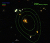 |
Fig. A.1. False color image of the COSMOS-Web ring and its environment with F115W and F150W in the blue channel, F277W in the green channel, and F444W in the red channel. SCUBA-2 detection contours at 850 μm are overlaid on top of the ring. |
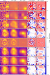 |
Fig. A.2. Morphology of the COSMOS-Web ring in the bluest bands. See the caption of Fig. 2 for the description. |
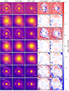 |
Fig. A.3. Morphology of the COSMOS-Web ring in the reddest bands. See the caption of Fig. 2 for the description. |
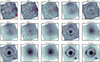 |
Fig. A.4. Cutouts of ×3″ of the Einstein ring in all bands. Images are sorted from the bluest to the reddest band going left to right and top to bottom. Each image is scaled using a square root function and ZScale intervals to enhance the contrast between the bright lens and the fainter surrounding ring. Contours from the detection image of SOURCEXTRACTOR++ are shown in all images as white lines. The circle with red dotted lines show the location of the nearby UV-bright contaminant discussed in Sect. 2.2 and in Fig. 5. North is up and east is to the left. |
All Tables
Photometric redshift estimates and physical properties of the source. For SE++, we quote the results on CW.
All Figures
|
Fig. 1. False color image of the COSMOS-Web ring made by cutouts from the HST/ACS F814W, JWST/NIRCam F115W, and F150W bands into the blue channel, the NIRCam F277W band into the green channel and the NIRCam F444W band into the red channel. The white bar in the bottom left represents the PSF FWHM in the F444W band. Two clumps CW and CE in the ring are identified in the figure. North is up and east is to the left. |
| In the text | |
|
Fig. 2. Morphology of the COSMOS-Web ring in the F444W (top row) and F115W (bottom row) bands. From left to right: 3″ × 3″ cutouts, best-fit lens model in image plane from SL_FIT, best-fit morphological model of the lens, CW, CE, and the nearby satellite with SOURCEXTRACTOR++, residuals from SL_FIT, and residuals from SOURCEXTRACTOR++. For each band, the same flux scale is applied for the both image and the models. All images have been projected on the same HST coordinate grid (north up and east left) with a scale of 0.06″ per pixel. In both F115W and F444W images, the critical line from SL_FIT’s best-fit mass model is shown as a white line. The PSF FWHM is indicated as a white bar in the bottom left corner of the cutouts and was derived on super-sampled PSF cutouts using one pixel-wide circular annuli. See Figs. A.2 and A.3 for all the bands. |
| In the text | |
|
Fig. 3. Source plane reconstructions from SL_FIT and PYAUTOLENS. Top row: gray-scale rendering of the SL_FIT reconstructed background source morphology in the F277W band on the left and false color representation on the right obtained by combining reconstructions of the source in the F444W (red channel), F277W (green channel), and F150W (blue channel) bands. Caustic lines are overlaid in red. Bottom row: source reconstruction from PYAUTOLENS in the JWST/NIRCam F115W band (left-hand plot) and in the F444W band (middle plot) bands using identical mass models. The right-hand plot represents the superposition of the two reconstructions with F115W in blue and F444W in red. In each panel, the caustic lines are shown. North is up and east is to the left. We note that, because of the mass-sheet degeneracy (e.g., Liesenborgs & De Rijcke 2012), the scales between the two source reconstructions cannot be directly compared. |
| In the text | |
|
Fig. 4. Results of the independent PYAUTOLENS lens model fits to the F115W, F150W, F277W, and F444W bands. From left to right: observed image, lens model image, normalized residual map, and source reconstruction. North is up and east is to the left. |
| In the text | |
|
Fig. 5. Results from SED fitting on the foreground lens and background source and their corresponding PDFs. Left: SED fitting results from LEPHARE for the lens (red) and the source (blue) using the photometry extracted from the lens modeling with SL_FIT (see Sects. 2.3 and 3). Right: redshift PDF for the lens and the source (same colors) when using LEPHARE (continuous lines), CIGALE (dashed lines), and EAZY (dotted lines). We note that the detections in the u, g, and r bands for the source are likely contaminated by a nearby UV-bright foreground galaxy located west of the ring (see Fig. A.4.) |
| In the text | |
|
Fig. 6. Comparison between the DM halo mass deduced from lensing and the theoretical value obtained from stellar-to-halo mass relations (SHMRs). Left: SHMR from Shuntov et al. (2022) (in orange) and Behroozi et al. (2013) (in teal) at z ∼ 2 that we use to estimate the dark matter halo mass in which the lens resides. The solid black horizontal line marks the total stellar mass that we estimate for the lens, while the dashed vertical orange and teal lines mark the halo mass obtained from Shuntov et al. (2022) and Behroozi et al. (2013) SHMR respectively. For comparison, we also show the SHMR points from van Dokkum et al. (2024) that we derive using their total stellar mass and the Behroozi et al. (2013) SHMR as shown in the solid blue marker. The transparent blue marker shows the stellar and halo masses quoted in van Dokkum et al. (2024). Right: relation between projected mass within the Einstein radius and total halo mass. The orange dashed line and shaded regions show the results from Shuntov et al. (2022) SHMR, while the teal thick and thin dashed lines show results and the lower limit on the uncertainty from Behroozi et al. (2013) SHMR. The purple thick line shows the dark matter mass derived as Mtot(< θEin)−M⋆(< θEin), while the thin one shows the total mass derived from the SL_FIT modeling. For comparison, we also show the results quoted in van Dokkum et al. (2024) in a dashed-dotted blue line. |
| In the text | |
|
Fig. 7. Inner slope γ of the total mass profile of the lens as a function of redshift for 44 strong lenses from Etherington et al. (2023) (blue points) and the high redshift lens studied by Wong et al. (2014) (green point). Independent values for the COSMOS-Web ring are shown for F115W (blue), F150W (cyan), F277W (orange), and F444W (red). |
| In the text | |
|
Fig. A.1. False color image of the COSMOS-Web ring and its environment with F115W and F150W in the blue channel, F277W in the green channel, and F444W in the red channel. SCUBA-2 detection contours at 850 μm are overlaid on top of the ring. |
| In the text | |
|
Fig. A.2. Morphology of the COSMOS-Web ring in the bluest bands. See the caption of Fig. 2 for the description. |
| In the text | |
|
Fig. A.3. Morphology of the COSMOS-Web ring in the reddest bands. See the caption of Fig. 2 for the description. |
| In the text | |
|
Fig. A.4. Cutouts of ×3″ of the Einstein ring in all bands. Images are sorted from the bluest to the reddest band going left to right and top to bottom. Each image is scaled using a square root function and ZScale intervals to enhance the contrast between the bright lens and the fainter surrounding ring. Contours from the detection image of SOURCEXTRACTOR++ are shown in all images as white lines. The circle with red dotted lines show the location of the nearby UV-bright contaminant discussed in Sect. 2.2 and in Fig. 5. North is up and east is to the left. |
| In the text | |
Current usage metrics show cumulative count of Article Views (full-text article views including HTML views, PDF and ePub downloads, according to the available data) and Abstracts Views on Vision4Press platform.
Data correspond to usage on the plateform after 2015. The current usage metrics is available 48-96 hours after online publication and is updated daily on week days.
Initial download of the metrics may take a while.