| Issue |
A&A
Volume 686, June 2024
|
|
|---|---|---|
| Article Number | A2 | |
| Number of page(s) | 18 | |
| Section | The Sun and the Heliosphere | |
| DOI | https://doi.org/10.1051/0004-6361/202449319 | |
| Published online | 24 May 2024 | |
Damped kink motions in a system of two solar coronal tubes with elliptic cross sections⋆
1
Shandong Provincial Key Laboratory of Optical Astronomy and Solar-Terrestrial Environment, Institute of Space Sciences, Shandong University, Weihai 264209, PR China
e-mail: This email address is being protected from spambots. You need JavaScript enabled to view it.
2
Centre for Mathematical Plasma Astrophysics, Department of Mathematics, KU Leuven, Celestijnenlaan 200B, 3001 Leuven, Belgium
Received:
23
January
2024
Accepted:
3
March
2024
Abstract
Aims. This study is motivated by observations of coordinated transverse displacements in neighboring solar active region loops, addressing specifically how the behavior of kink motions in straight two-tube equilibria is impacted by tube interactions and tube cross-sectional shapes.
Methods. We worked with linear, ideal, pressureless magnetohydrodynamics. Axially standing kink motions were examined as an initial value problem for transversely structured equilibria involving two identical, field-aligned, density-enhanced tubes with elliptic cross sections (elliptic tubes). Continuously nonuniform layers were implemented around both tube boundaries. We numerically followed the system response to external velocity drivers, largely focusing on the quasi-mode stage of internal flows to derive the pertinent periods and damping times.
Results. The periods and damping times that we derive for two-circular-tube setups justify the available modal results found with the T-matrix approach. Regardless of cross-sectional shapes, our nonuniform layers feature the development of small-scale shears and energy accumulation around Alfvén resonances, indicative of resonant absorption and phase mixing. As with two-circular-tube systems, our configurational symmetries still make it possible to classify lower-order kink motions by the polarization and symmetric properties of the internal flows; hence, such motions are labeled as Sx and Ax. However, the periods and damping times for two-elliptic-tube setups further depend on cross-sectional aspect ratios, with Ax motions occasionally damped less rapidly than Sx motions. We find uncertainties up to ∼20% (∼50%) for the axial Alfvén time (the inhomogeneity lengthscale) if the periods (damping times) computed for two-elliptic-tube setups are seismologically inverted with canonical theories for isolated circular tubes.
Conclusions. The effects of loop interactions and cross-sectional shapes need to be considered when the periods, and in particular the damping times, are seismologically exploited for coordinated transverse displacements in adjacent coronal loops.
Key words: methods: numerical / Sun: corona / Sun: magnetic fields
Movies associated to Figs. 6 and 10 are available at https://www.aanda.org.
© The Authors 2024
 Open Access article, published by EDP Sciences, under the terms of the Creative Commons Attribution License (https://creativecommons.org/licenses/by/4.0), which permits unrestricted use, distribution, and reproduction in any medium, provided the original work is properly cited.
This article is published in open access under the Subscribe to Open model. This email address is being protected from spambots. You need JavaScript enabled to view it. to support open access publication.
1. Introduction
Cyclic transverse displacements of solar coronal loops are arguably the most extensively observed collective motion in modern solar coronal seismology (see e.g., Nakariakov & Kolotkov 2020; Nakariakov et al. 2021, for recent reviews). Two regimes have been established. The decayless regime is such that the displacements show little damping and their magnitudes are usually substantially smaller than visible loop widths, with both features already clear when this regime was first identified in measurements with Hinode (Tian et al. 2012) and the Solar Dynamics Observatory/Atmospheric Imaging Assembly (SDO/AIA; Wang et al. 2012; Nisticò et al. 2013; Anfinogentov et al. 2013). This regime is known to be unconnected with eruptive events but ubiquitous in active region (AR) loops, as is evidenced by a statistical survey of the SDO/AIA data (Anfinogentov et al. 2015) and by the recent series of analyses of the measurements with the Extreme Ultraviolet Imager (EUI) on board the Solar Orbiter (e.g., Zhong et al. 2022, 2023; Petrova et al. 2023). Decaying loop displacements, on the other hand, typically damp over several cycles and are of larger amplitudes, as was revealed by their first imaging observations by the Transition Region and Coronal Explorer (TRACE; Schrijver et al. 1999; Aschwanden et al. 1999; Nakariakov et al. 1999). These decaying motions are usually associated with lower coronal eruptions (Zimovets & Nakariakov 2015). Regardless, there exist ample detections of decaying displacements, an inexhaustive list being those by Hinode (Ofman & Wang 2008; Van Doorsselaere et al. 2008a; Erdélyi & Taroyan 2008), the Solar TErrestrial RElations Observatories (STEREO; Verwichte et al. 2009), and SDO/AIA (Aschwanden & Schrijver 2011; White & Verwichte 2012). It has therefore proven possible to conduct statistical studies, either by compiling published results (e.g., Verwichte et al. 2013) or by directly cataloging the SDO/AIA events (Goddard et al. 2016; Nechaeva et al. 2019). Decaying cyclic displacements were specifically established to be nearly exclusively axial fundamentals (e.g., Fig. 9 in Goddard et al. 2016 and Fig. 5 in Nechaeva et al. 2019).
Seismological applications of cyclic transverse displacements typically start with their identification as trapped fast kink motions. Practically, this identification largely relies on the scheme for classifying collective motions in straight, static, field-aligned configurations in which isolated density-enhanced tubes with circular cross sections (circular tubes hereafter) are embedded in an otherwise uniform corona (Edwin & Roberts 1983, hereafter ER83; also Zajtsev & Stepanov 1975; Cally 1986). That the configuration is structured only transversely and in a one-dimensional (1D) manner means that the azimuthal wave number, m, makes physical sense, with kink motions corresponding to m = 1 (see the textbooks by Roberts 2019; Goedbloed et al. 2019). Let “ER83 equilibria” label specifically those in which the transverse structuring is piecewise constant. The relevant theories then enable the measured periods of axially standing kink motions to be employed to infer the axial Alfvén time, and hence the coronal magnetic field strength for decayless (e.g., Anfinogentov & Nakariakov 2019; Li & Long 2023) and decaying regimes alike (Nakariakov & Ofman 2001; also the reviews by e.g., Nakariakov & Verwichte 2005; De Moortel & Nakariakov 2012; Nakariakov et al. 2021). While undamped for ER83 equilibria, trapped fast kink motions are in general resonantly absorbed in the Alfvén continuum when the 1D structuring is allowed to be continuous (Ruderman & Roberts 2002; Goossens et al. 2002, and references therein). Theoretically, the concept of kink quasi-modes then arises and the internal kink motions are damped in conjunction with the accumulation and phase mixing of localized Alfvénic motions (e.g., Poedts & Kerner 1991; Tirry & Goossens 1996; Soler et al. 2013; also the review by Goossens et al. 2011). Seismologically, resonant absorption has been customarily invoked to interpret the decay of large-amplitude loop displacements, thereby allowing the measured damping times to be employed to deduce such key parameters as the transverse inhomogeneity lengthscales (e.g., Aschwanden et al. 2003; Goossens et al. 2008; Arregui & Asensio Ramos 2011; Arregui et al. 2015; Arregui 2022).
Deviations from the canonical ER83 equilibria are known to impact the behavior of collective motions, and we choose to focus on two geometrical properties that render the meaning of the azimuthal wave number less clear (e.g., the review by Li et al. 2020). One concerns loop cross sections, which may actually be tied to coronal heating via their key role in determining the morphology of coronal loops in, say, soft X-ray (Klimchuk et al. 1992) and extreme ultraviolet (EUV; Watko & Klimchuk 2000) in the first place. Recent imaging observations with Hi-C (Klimchuk & DeForest 2020) and Hi-C 2.1 (Williams et al. 2021) suggest that AR loops may maintain a circular cross section throughout their visible segments. However, there also exist suggestions that favor elliptic cross sections to better account for the morphology of AR loops, as deduced with the aid of coronal magnetic field modeling (e.g., Wang & Sakurai 1998; Malanushenko & Schrijver 2013) and/or multi-vantage-point measurements with STEREO (e.g., McCarthy et al. 2021). In particular, the derived aspect ratios may readily attain ∼1.5 − 5 (Malanushenko & Schrijver 2013), a range also compatible with the spectroscopic measurements with the Hinode/EUV Imaging Spectrometer (EIS; Kucera et al. 2019). We restrict ourselves to straight configurations in which coronal loops preserve a constant elliptic cross section along their axes (elliptic tubes hereafter). Substantial attention has been paid to collective perturbations in such equilibria from both the modal (e.g., Ruderman 2003; Erdélyi & Morton 2009; Morton & Ruderman 2011; Aldhafeeri et al. 2021) and initial value problem (IVP) perspectives (Guo et al. 2020). Despite the lack of axisymmetry, kink motions remain identifiable as those that transversely displace the tube axes, and in general they remain subjected to resonant absorption for continuous transverse structuring. However, as was first shown by Ruderman (2003), one now needs to discriminate between two distinct polarizations, where the internal flows are primarily directed along the major (“major-polarized” for brevity) and minor axes (“minor-polarized”), respectively. In addition, the periods of major-(minor-) polarized kink motions increase (decrease) with the major-to-minor-axis ratio, while the damping times for both polarizations tend to increase with this ratio. It was further demonstrated that the density contrast between elliptic tubes and their surrounding fluids plays a subtle role in mediating the differences between the dispersive properties of the differently polarized motions (Guo et al. 2020).
Another geometric property pertains to systems involving multiple tubular structures. Observationally, it has long been known that perturbations in such systems may evolve collectively, an incomplete list of examples being the coordinated transverse displacements detected either in groups of prominence threads (e.g., Yi et al. 1991; Lin et al. 2003; Okamoto et al. 2007; also the review by Arregui et al. 2018) or in neighboring AR loops (e.g., Schrijver & Brown 2000; Schrijver et al. 2002; Verwichte et al. 2004; Wang et al. 2012; White et al. 2013). Kink motions in straight multi-circular-tube systems have also been extensively examined theoretically. We choose to concentrate on the modal analyses where a harmonic time-dependence is assumed a priori, noting that multidimensional IVP studies prove equally informative (e.g., Terradas et al. 2008a; Ofman 2009; Magyar & Van Doorsselaere 2016; Guo et al. 2019a). The first modal examination was due to Luna et al. (2008, hereafter L08), who numerically solved the pertinent eigenvalue problem (EVP) for undamped kink modes in a two-tube system. Broadly speaking, two different approaches have been employed in further modal studies. The ensuing EVPs turn out to be analytically tractable in the thin-tube (TT) limit for two-tube equilibria when formulated in bicylindrical coordinates, for both undamped (Van Doorsselaere et al. 2008b; Robertson et al. 2010; Ruderman & Petrukhin 2023) and damped kink motions (Robertson & Ruderman 2011; Gijsen & Van Doorsselaere 2014). Similar EVPs have also been formulated with the T-matrix formalism of scattering theory, originally introduced to solar contexts by Bogdan & Zweibel (1985, 1987). This formalism is sufficiently general for examining kink motions in composite equilibria comprising an arbitrary number of circular tubes, with specific investigations available for undamped motions in systems with two or three (Luna et al. 2009) or even up to tens of tubes (Luna et al. 2010, 2019). Addressing continuous transverse structuring, the T-matrix approach proves capable of handling the resonant absorption of collective motions in general (Keppens et al. 1994) and particularly that of kink motions in two-tube equilibria (Soler & Luna 2015, hereafter SL15). The damping is nonetheless assumed to be weak by construction, given that it was incorporated in the T-matrix framework exclusively via the thin-boundary (TB) connection formulae (see SL15 for more details; also see Sakurai et al. 1991 for the first derivation of the TB formulae). Regardless, kink motions are known to be much more complicated in multi-tube equilibria than in isolated circular tubes, and we restrict ourselves to two-identical-tube systems. It was shown by L08 (see Fig. 2 therein) that kink motions, namely those that displace both tube axes, need to be classified according to both the polarization and symmetric properties of the two internal flows. Such mode labels as Sx, Ax, Sy, and Ay then ensue, one subtlety being that the Sx − Ay and Ax − Sy pairs become indistinguishable in terms of frequencies (Van Doorsselaere et al. 2008b) and damping rates (SL15) when the tubes are sufficiently thin. This subtlety notwithstanding, Ax motions always turn out to oscillate and damp more rapidly than Sx motions: the differences between the frequencies and in particular the damping rates may be substantial enough to impact seismological deductions (see Fig. 4 in SL15).
This study is intended to examine damped lower-order kink motions in a two-identical-elliptic-tube system, thereby addressing the situation in which neither the equilibrium configuration as a whole nor an individual tube causes the azimuthal wave number to make exact sense. We adopt linear, pressureless, ideal magnetohydrodynamics (MHD) throughout, given that quiescent AR loops are of primary interest. We also adopt an IVP perspective, paying particular attention to the frequencies and damping rates of axially standing motions by largely focusing on the duration where the concept of quasi-modes applies. Our study is new in the following two respects. Firstly, two-elliptic-tube systems have yet to be explored in the context of collective waves, meaning that our study sheds new light on how the dispersive properties of kink motions are impacted by the joint effects of tube interactions and tube cross-sectional shapes. When applied to seismological contexts, our results can therefore help assess the uncertainties in the key physical parameters that one deduces with the customary practice in which the joints effects are absent. Secondly, there exist no IVP studies dedicated to the dispersive properties of damped kink motions in two-tube systems to our knowledge. Our numerical analysis, conducted with a self-developed code, therefore helps to verify the T-matrix results obtained by SL15.
The outline of this manuscript is as follows. Section 2 offers the mathematical formulation of our IVP together with a description of our numerical code. We then focus on circular tubes in Sect. 3, testing our code outputs against available results obtained with independent approaches. Section 4 proceeds to present our numerical results for two-elliptic-tube systems. Section 5 discusses some seismological implications of this study. Our findings are summarized in Sect. 6, where some concluding remarks are also given.
2. Problem formulation and solution method
2.1. Governing equations
We adopted pressureless, ideal MHD as our theoretical framework, in which the primitive dependents are the mass density, ρ, velocity, v, and magnetic field, B. We let (x, y, z) be a Cartesian system, and let the equilibrium quantities be denoted with a subscript, 0. We took the equilibrium magnetic field to be uniform and z-directed (B0 = B0ez). Only straight, static, field-aligned configurations were of interest, meaning that v0 = 0 and the structuring is encapsulated in ρ0(x, y). The Alfvén speed vA was defined by  , where μ0 is the magnetic permeability of free space. With magnetically closed structures in mind, we placed two dense photospheres at z = 0 and z = L.
We formulated an IVP to examine how our equilibrium responds to small-amplitude perturbations (denoted by subscript 1). It follows from linearized, ideal, pressureless MHD equations that
 (1)
(1)
 (2)
(2)
 (3)
(3)
 (4)
(4)
 (5)
(5)
We focused on axially standing motions by adopting the ansatz
 (6)
(6)
where k = nπ/L is the quantized axial wave number (n = 1, 2, …). Equations (1)–(5) then become
 (7)
(7)
 (8)
(8)
 (9)
(9)
 (10)
(10)
 (11)
(11)
Axial fundamentals (k = π/L) were examined throughout, even though our analysis can be readily adapted to any axial harmonic number, n.
2.2. Energy conservation law
Energetics considerations turn out to be necessary. Consider a volume, V, that laterally occupies an arbitrary area, Q, and is axially bounded by the planes z = 0 and z = L. Let the curve enclosing Q be denoted by ∂Q. Let [en, et, ez] further define a right-handed set of orthonormal system at any point along ∂Q, with the normal direction, en, pointing away from Q. An energy conservation law can be readily derived from Eqs. (1)–(5), reading
 (12)
(12)
where
 (13)
(13)
 (14)
(14)
 (15)
(15)
It should be noted that the ansatz Eq. (6) was employed, and that  is connected with the Eulerian perturbation of total pressure. It should also be noted that dlt denotes the elementary arclength in the tangential direction defined by et. When multiplied by L/2, the symbols E and F represent the instantaneous perturbation energy in V and the net energy flux out of V, respectively. We nonetheless refer to E (F) as the total energy (the net energy flux) for brevity. Likewise, the symbol ϵ in Eqs. (13) and (15) is referred to as the energy density. We also drop the hat symbol in what follows.
2.3. Equilibrium configuration and initial perturbation
Our equilibrium comprises a composite structure embedded in an otherwise uniform external corona (denoted by the subscript e). By “composite” we mean two identical tubes with elliptic cross sections and separated by d. j labels a tube, and a two-dimensional (2D) position vector, Xj = (Xj, Yj), denotes the center of tube j. The tube centers were placed on the x axis without loss of generality, enabling a tube to be referred to as either the left tube (j = L) or the right one (j = R). The tube centers were further taken to be symmetric about x = 0, resulting in XL, R = ∓d/2 and YL, R = 0. We consistently use subscript i to denote the equilibrium quantities at either tube axis, meaning in particular that the internal density and Alfvén speed are denoted by ρi and vAi, respectively. Likewise, by vAe we denote the Alfvén speed evaluated with the external density ρe.
Our two-tube structure is characterized as follows. The tubes are taken to be identical not only in cross-sectional shapes but in their orientations relative to the x axis. For simplicity, we considered only two orientations by discriminating between whether the major axis (hereafter “x-major”) or the minor one (“x-minor”) of a tube aligns with the x direction. We made ax and ay denote the spatial extent that a tube spans in the x and y directions, respectively. The x-major (x-minor) orientation then means that ax > ay (ax < ay). Both orientations are realized by the density distribution (j = L or R),
 (16)
(16)
with the intermediate dimensionless variable,  , defined by
 (17)
(17)
We took d ≥ 2ax such that the tube, j, can be unambiguously identified as where  . We also used a (b) to denote the semi-major (semi-minor) axis, meaning that [ax = a, ay = b] ([ax = b, ay = a]) for the x-major (x-minor) orientation. The symbol b was favored when the limiting case of circular tubes was examined (a = b). Equation (16) represents a tube profile that continuously connects the internal density, ρi, to the external one, ρe, via some elliptic layer of width,
  (
( ), in the direction of the major (minor) axis. When a = b, this profile is equivalent to the sinusoidal distribution introduced by Ruderman & Roberts (2002, hereafter RR02) for modeling circular inhomogeneities (see e.g., Van Doorsselaere et al. 2004; Soler et al. 2013; Chen et al. 2021, for more applications). Somewhat subtle is that the RR02 implementation of a tube centered at (Xj, 0) reads as
 (18)
(18)
Here,  . Evidently, the geometrical parameters, [ℛ, ℓ], characterizing the RR02 implementation are connected to ours via
 (19)
(19)
Our equilibrium configuration, illustrated in Fig. 1b, is a straightened version of a composite system in which two tubes are separated in the x direction and anchored in the photosphere (Fig. 1a). We see the x (y) direction in Fig. 1b as horizontal (vertical) given that the y − z plane can be identified as the tube plane. For two-tube systems, however, it turns out to also be necessary to classify lower-order kink motions into Sx, Ax, Sy, and Ay types by combining the symmetric and polarization properties of the internal flow fields (see Fig. 2 in L08). Proposed for two-identical-circular-tube systems, the subscript x (y) arises when the internal velocities are dominated by their x (y) components, while the symbol, S (A), is such that the dominant internal velocity component is symmetric (antisymmetric) about x = 0. This classification is expected to carry over when elliptic tubes are examined. Somewhat complicated is that one needs to distinguish between the x-major and x-minor arrangements (Figs. 1c and d), meaning for instance that the frequencies of the Sx motions are likely to be different for different tube orientations.
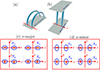 |
Fig. 1. Schematics showing both the two-elliptic-tube configuration and lower-order kink motions therein. Illustrated in (b) are two identical tubes that have elliptic cross sections and that are separated in the x direction. The y − z plane is identified as the tube plane, the meaning of which is clearer in the curved representation in panel a. This study examines only two tube orientations (panels c and d), with the one labeled “x-major” (“x-minor”) corresponding to the situation where the major (minor) axis of either tube is aligned with the x axis. The tube centers are placed symmetrically with respect to the y axis. Only axial fundamentals are considered, making it possible to examine the three-dimensional (3D) wave fields with a 2D approach. Lower-order kink motions are classified according to their internal flow fields in the apex plane (panels c or d); hence, such symbols as Sx and Ay (see the text for more details). |
Our equilibrium is perturbed via velocities. We considered only Sx and Ax motions, given that kink motions are commonly observed to be horizontally polarized (see Zhong et al. 2023 and references therein; see e.g., Wang et al. 2008; Aschwanden & Schrijver 2011 for observational instances of vertical kink motions). Regardless of tube orientations, these are excited by imposing
![Mathematical equation: $$ \begin{aligned} \dfrac{\boldsymbol{v}_{\rm ini}(x,{ y})}{v_{\mathrm{Ae}}} = \mathrm{e}^{4} \left\{ \exp \left[-\left(\dfrac{x+x_{\rm ini}}{b}\right)^2\right] \pm \exp \left[-\left(\dfrac{x-x_{\rm ini}}{b}\right)^2\right]\right\} {\boldsymbol{e}}_{x}, \end{aligned} $$](/articles/aa/full_html/2024/06/aa49319-24/aa49319-24-eq27.gif) (20)
(20)
where xini = XR + ax + 2b, and we recall that [XR = d/2, b = min(ax, ay)]. The coefficient, e4, is introduced only for plotting purposes, the magnitude being immaterial for linear studies. Equation (20) represents a pair of planar compressible perturbations concentrated in the ambient corona, exciting Sx (Ax) motions when the plus (minus) sign applies.
2.4. Parameter overview and solution method
The behavior of small-amplitude perturbations is determined by two sets of parameters. We took the dimensional set to be {ρe, b, vAe}, which serve merely as normalizing constants in our context. We accept that we are primarily interested in such timescales as the oscillation period and damping time. The importance of the dimensionless set then follows from a straightforward dimensional analysis, which dictates that a timescale, tscale, is formally expressible as
![Mathematical equation: $$ \begin{aligned} \dfrac{v_{\mathrm{Ae}} t_{\rm scale}}{b} = \mathcal{F} \left[\mathrm{orientation}, \dfrac{\rho _{\mathrm{i}}}{\rho _{\mathrm{e}}}, \dfrac{a}{b}, \bar{l}, \dfrac{d}{b}; \; kb; \; \mathrm{perturbation\,pattern}\right]. \end{aligned} $$](/articles/aa/full_html/2024/06/aa49319-24/aa49319-24-eq28.gif) (21)
(21)
The subgrouped parameters characterize the transverse structuring, axial wave number, and initial perturbation, respectively. By “orientation” we refer to either “x-major” or “x-minor”. By “perturbation pattern” we mean either Sx or Ax. We fixed the axial wave number at kb = π/30 throughout, meaning a tube length of L = 30b for axial fundamentals. This L/b suffices for our purposes, lying toward the lower end but within the accepted range for AR loops imaged in the EUV (e.g., Aschwanden et al. 2004; Schrijver 2007). Table 1 briefly overviews our computations, which are grouped into four sets to be detailed later. The density contrast, ρi/ρe, was fixed at either 3 or 5, both values being representative of AR loops (e.g., Aschwanden et al. 2004, and references therein).
Summary of time-dependent solutions presented in the text.
We solved Eqs. (7)–(11) with the following procedure. A computational domain, [ − xM, xM]×[−yM, yM], was discretized into a uniform mesh with identical spacing in the x and y directions (Δx = Δy = Δ). The zero-gradient condition was implemented for all unknowns at all boundaries. We evolved Eqs. (7)–(11) with the classic MacCormack scheme (MacCormack 1969), a popular finite-difference algorithm that is second-order accurate in both space and time (see the textbooks by, e.g., Anderson 1995; Jardin 2010, for more). The time step, Δt, was set via an effective Courant number, c := (vAeΔt/Δx)2/3 + (vAeΔt/Δy)2/3, inspired by Hong (1996). A value of c = 0.99 was employed for all the presented results. We have verified that varying c between ∼0.7 and ∼1.3 introduces no discernible difference, and numerical stability is consistently maintained.
Some remarks on the grid setup are necessary. We start by noting that the spatial spacing, Δ, restricts the time frame in which numerical solutions make physical sense, an aspect raised by Terradas et al. (2008a, hereafter T08), who numerically solved an equivalent set of governing equations. Defining the Alfvén frequency ωA(x, y) = kvA(x, y), one expects that some time-dependent phase-mixing length will emerge as (Mann et al. 1995)
 (22)
(22)
which characterizes the transverse lengthscales of resonantly generated Alfvénic motions in the nonuniform portions in the system. It suffices to consider only the nonuniform layer of one tube. Evidently, the shortest phase-mixing length,  , at a given instant occurs at the strongest |∇ωA(x, y)|. Equally evident is that this strongest |∇ωA(x, y)| depends only on ρi/ρe and
  even when elliptic tubes are examined. Let
  denote
  at t = 500b/vAe, before which our computations are consistently terminated. It then follows from the arguments by T08 that our signals are physically relevant provided
  . As is shown by Table 1, this criterion is satisfied by the reference grid setup for any set of our computations.
3. Test computations for circular tubes
The MacCormack scheme, while a textbook one, has not been applied to Eqs. (7)–(11). Its applicability is therefore examined in this section via some test computations for which the time-dependent behavior can be established or expected with independent methods. Only circular tubes are of interest, and we refer to b(=a) as our tube radius. We started by examining the response of a one-circular-tube system to axisymmetric (sausage) perturbations, following our previous study (Li et al. 2022) to formulate both the equilibrium and the initial perturbation. The Fourier-integral-based solutions, presented in Fig. 4 therein, agree closely with our MacCormack solutions. In particular, no discernible numerical anisotropy shows up even though finite differences were performed on a Cartesian grid to examine a nonplanar equilibrium (see e.g., the review by Sescu 2015, for more on numerical anisotropy). The rest of this section focuses on kink perturbations.
3.1. Kink motions in a one-circular-tube setup
This subsection examines kink perturbations in a one-circular-tube configuration, placing the tube center at the origin without loss of generality. The equilibrium density is realized through Eq. (16) by taking [ax = ay = b, Xj = 0] and then dropping the subscript j. Kink motions in such a configuration have been extensively studied (see the review by Nakariakov et al. 2021, and references therein), readily allowing our MacCormack computations to be compared with known results. By “known” we refer to two sets of studies. Set one, presented in Sect. 4 of T08, adopts the RR02 implementation to examine the system response to an initial perturbation of the form
![Mathematical equation: $$ \begin{aligned} \boldsymbol{v}_{\rm ini}(x,{ y}) = v_{\mathrm{Ae}} \exp \left[-\dfrac{({ y}-{ y}_{\rm ini})^2}{\sigma ^2}\right] {\boldsymbol{e}}_{{ y}}. \end{aligned} $$](/articles/aa/full_html/2024/06/aa49319-24/aa49319-24-eq37.gif) (23)
(23)
Figure 2 in T08 then presents the time sequence of vy sampled at the tube center for a combination of parameters, [ρi/ρe = 3, kℛ = π/20, ℓ/ℛ = 0.6], and [yini = 3ℛ, σ = ℛ]. We repeated the same experiment, using Eq. (19) to address notational differences and adopting an identical computational grid. Our finite-difference results are found to be consistent with T08, despite the numerical code therein adopting the finite-volume methodology.
We proceeded to perform an additional series of computations to examine whether our code outputs agree with expectations for ideal kink quasi-modes. We let ω = Ω − iγ denote the complex-valued quasi-mode frequency, and saw Ω and γ as positive. With the kink speed, ckink, defined as
 (24)
(24)
it is well established that (RR02; see also Goossens et al. 1992; Soler et al. 2013)
 (25)
(25)
in the so-named thin-tube-thin-boundary limit (TTTB, kb ≪ 1 and  ). We note that the TTTB expressions are usually formulated in terms of the RR02 notations [ℛ, ℓ]. We also note that the TTTB results may not hold up well beyond their range of applicability (e.g., Soler et al. 2014; Yu et al. 2021). We therefore also evaluated the mode frequencies numerically with the general-purpose finite-element code PDE2D (Sewell 1988), computing ideal kink quasi-modes as resistive eigenmodes (see Goossens et al. 2011 for conceptual clarifications; see also Terradas et al. 2005 for the first introduction of PDE2D to solar contexts)1. No restriction was necessary for kb or
  .
.
The rest of this subsection is devoted to a fixed combination, [ρi/ρe = 3, kb = π/30], allowing only  to vary. Furthermore, the reference grid (see Table 1) is consistently employed in our time-dependent computations, where kink motions are excited by a perturbation of the fixed form
![Mathematical equation: $$ \begin{aligned} \dfrac{\boldsymbol{v}_{\rm ini}(x,{ y})}{v_{\mathrm{Ae}}} = \mathrm{e}^{4} \exp \left[-\dfrac{(x+3b)^2}{b^2}\right] {\boldsymbol{e}}_{x}. \end{aligned} $$](/articles/aa/full_html/2024/06/aa49319-24/aa49319-24-eq43.gif) (26)
(26)
Equation (26) is essentially identical to Eq. (23) except that vx rather than vy is perturbed. Figure 2a examines a representative case with  , showing the temporal evolution of the x speed sampled at the tube center (vx(0, 0, t), the solid curve). This vx signal is seen to feature some rapid variations for t ≲ 15b/vAe. By “rapid” we mean timescales on the order of the transverse Alfvén time (b/vAi), which derives from the multiple reflections off the tube boundaries of the perturbations that are imparted by the external driver to the tube. The vx signal transitions toward a regular, more slowly varying pattern afterward, becoming monochromatic when t ≳ 70b/vAe. We chose to leave out the first extremum in this stage for safety, and fit the segment encompassing the next six (the red asterisks) with an exponentially damped cosine,
 (27)
(27)
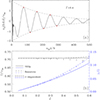 |
Fig. 2. Kink motions in isolated tubes with circular cross sections for a fixed pair of density contrast and dimensionless axial wave numbers, [ρi/ρe = 3, kb = π/30]. A specific dimensionless layer width, |


The damping envelope from the best fit is plotted for the entire duration in Fig. 2 with the dashed curves. One sees that this best-fit envelope, while derived for some segments, offers a good description of the longer-scale behavior as well (say, t ≳ 300b/vAe).
Figure 2b surveys a range of  by plotting the oscillation frequencies (Ωfit, the open black circles) and damping rates (γfit, blue), which are translated from the best-fit periods and damping times (Ωfit = 2π/Pfit and γfit = 1/τfit). We note that Ω is measured in units of the external Alfvén frequency, ωAe = kvAe, and γ/Ω is presented rather than γ itself. The curves in Fig. 2b further provide the quasi-mode expectations with either the analytical TTTB expression (Eq. (25), the solid lines) or the PDE2D computations (labeled “Resistive”, dashed lines). One sees that the TTTB results provide a rather good approximation to the numerical “Resistive” ones, the frequencies being practically the same and the damping rates differing by ≳10% only when
  . One further sees that the open circles agree well with the “Resistive” computations, demonstrating that the internal flow fields practically evolve as an ideal quasi-mode, at least in the interval where the fitting was performed.
3.2. Kink motions in a two-circular-tube setup
This subsection examines kink motions in a two-circular-tube configuration, for which the distinction between Sx and Ax patterns becomes necessary. The initial perturbation was therefore chosen to follow Eq. (20), where xini evaluates to d/2 + 3b. Our code consistently adopted ![Mathematical equation: $ [b, \bar{l}] $](/articles/aa/full_html/2024/06/aa49319-24/aa49319-24-eq50.gif) notations. However, the mixed usage of the RR02 convention, [ℛ, ℓ], turned out to be necessary. The reason is that this RR02 convention was adopted by SL15 to examine ideal quasi-modes from an EVP perspective in a configuration physically identical to ours. Briefly put, the study by SL15 is based on the TB-embedded T-matrix formalism of scattering theory, the pertinent results being most straightforward for our time-dependent computations to be compared with. By “pertinent” we specifically refer to Fig. 4 therein, which presents the ℓ/ℛ-dependencies of the quasi-mode frequencies and damping rates for a fixed combination, [ρi/ρe = 5, d/ℛ = 2.5, kℛ = π/100]. Varying ℓ/ℛ actually impacts our
notations. However, the mixed usage of the RR02 convention, [ℛ, ℓ], turned out to be necessary. The reason is that this RR02 convention was adopted by SL15 to examine ideal quasi-modes from an EVP perspective in a configuration physically identical to ours. Briefly put, the study by SL15 is based on the TB-embedded T-matrix formalism of scattering theory, the pertinent results being most straightforward for our time-dependent computations to be compared with. By “pertinent” we specifically refer to Fig. 4 therein, which presents the ℓ/ℛ-dependencies of the quasi-mode frequencies and damping rates for a fixed combination, [ρi/ρe = 5, d/ℛ = 2.5, kℛ = π/100]. Varying ℓ/ℛ actually impacts our  , d/b, and kb simultaneously (see Eq. (19)). We adopted a fixed kb = π/30 to save computational time. This does not matter because we measure our timescales or frequencies in appropriate units (say, Ω in ωAe) and the resulting readings do not depend on kℛ when kℛ ≲ π/20 (see Fig. 3 in SL15, and note that kℛ < kb). Equation (19) readily converts the pair, [ℓ/ℛ, d/ℛ], into our
 ![Mathematical equation: $ [\bar{l}, d/b] $](/articles/aa/full_html/2024/06/aa49319-24/aa49319-24-eq52.gif) .
.
We tested our time-dependent computations against the SL15 results, to be labeled “T-matrix” for clarity. It sufficed to examine the time sequences of the x speed sampled at the left tube center (namely, vx(−d/2, 0; t)); the right counterpart is either identical (for Sx) or different only in sign (for Ax). Figure 3 focuses on the choice, ℓ/ℛ = 0.4, and plots the sampled vx for (a) the Sx and (b) the Ax patterns with the solid curves. The same analysis as in Fig. 2a was then repeated for both curves, whereby we singled out the six extrema (the red asterisks in Fig. 3) after the transitory phase to perform a fitting with Eq. (27). The best-fit exponential envelope, plotted by the dashed curves for the entire duration, is seen to reflect well the damping of kink motions for a much longer time.
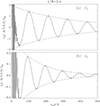 |
Fig. 3. Kink motions with (a) Sx and (b) Ax patterns in a two-circular-tube configuration. Plotted are the time sequences of the x speed sampled at the left tube center (vx(−d/2, 0; t), the solid curves) together with the best-fit damping envelopes (dashed). The time-dependent computations pertain to a fixed combination, [ρi/ρe = 5, ℓ/ℛ = 0.4, d/ℛ = 2.5, kb = π/30], with ℓ and ℛ being the nonuniform layer width and mean tube radius implemented by Ruderman & Roberts (2002), respectively. A fitting procedure with an exponentially damped cosine was performed over the duration exactly encompassing the extrema indicated by the red asterisks, even though the best-fit envelopes are plotted for the entire time interval. Kink motions are excited with the perturbation described by Eq. (20) with appropriate signs. |
Figure 4 proceeds to examine the ℓ/ℛ-dependencies of (a) the oscillation frequencies (Ω in ωAe) and (b) the damping-rate-to-frequency ratios (γ/Ω). The Sx and Ax patterns are distinguished with different colors. We present the best-fit values from our time-dependent computations with open circles, and overplot the T-matrix results with solid curves for comparison. These T-matrix curves are taken from Fig. 4 of SL15. Our best-fit results are seen to compare favorably with the T-matrix results, which is particularly true when ℓ/ℛ ≲ 0.3. This statement holds despite the somewhat visible difference in Ω at, say, ℓ/ℛ = 0.2, where the best-fit value actually deviates from its T-matrix counterpart by only ∼2.7%. One further sees that the most significant departure occurs for the Ax damping rate when ℓ/ℛ = 0.4. However, this difference is rather modest and reads as ∼21.7% in relative terms. We therefore conclude that the dispersive properties of kink quasi-modes can be reasonably computed by incorporating the shortcut TB formulae in the T-matrix framework for all ℓ/ℛ examined here2. Our time-dependent results, on the other hand, further corroborate the SL15 conclusion that Ax motions posses higher frequencies and damp more rapidly than Sx ones.
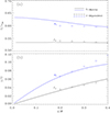 |
Fig. 4. Comparison of (a) the oscillation frequencies, Ω, and (b) the damping rates, γ, of ideal quasi-modes deduced from time-dependent computations (the open circles) with those expected with the T-matrix formalism (solid lines). We depict the results for the Sx and Ax patterns with different colors. The T-matrix curves are taken from Fig. 4 of Soler & Luna (2015, SL15). Shown here is how Ω and γ/Ω depend on ℓ/ℛ, while the rest of the parameters are fixed at [ρi/ρe = 5, d/ℛ = 2.5, kb = π/30]. The [ℓ/ℛ, d/ℛ] notations follow from SL15 for ease of comparison. |
3.3. Interim summary of the numerical aspects
This subsection further justifies our numerical treatment. An additional series of computations were performed to address the effects of the grid spacing, Δ, and the domain size, [xM, yM]. These results are collected in Appendix A to streamline the main text. Overall, we have verified that the MacCormack scheme is appropriate for our purposes, with no issue arising from the application to nonplanar structures of the finite-difference methodology on a Cartesian grid. The zero-gradient boundary condition is somehow not fully transparent to perturbations excited by our planar drivers, and the domain size somehow impacts how the internal flows transition to a quasi-mode behavior. However, this domain size effect is practically negligible on the best-fit periods (Pfit) and damping times (τfit) that we derive for the quasi-mode stage. Likewise, the computed internal flows are not affected by the grid spacing, Δ, provided that Δ is sufficiently small.
4. Kink motions in a two-elliptic-tube setup
This section is devoted to kink motions in a two-elliptic-tube configuration, for which the x-major and x-minor orientations need to be discriminated. The reference grid ([xM = 30b, yM = 25b, Δ = 0.01b], see Table 1) is consistently adopted, enabling a meaningful comparison between the tube orientations. The notations ![Mathematical equation: $ [a, b, \bar{l}] $](/articles/aa/full_html/2024/06/aa49319-24/aa49319-24-eq53.gif) are adopted throughout this section, where all computations pertain to a fixed combination of physical parameters,
are adopted throughout this section, where all computations pertain to a fixed combination of physical parameters, ![Mathematical equation: $ [\rho_{\mathrm{i}}/\rho_{\mathrm{e}}=3, \bar{l}=0.4, kb=\pi/30] $](/articles/aa/full_html/2024/06/aa49319-24/aa49319-24-eq54.gif) . We adjust only the dimensionless tube separation (d/b) and the ratio of the semi-major to semi-minor axis (a/b) for a given orientation and a given perturbation pattern (see Eq. (21)). Tube overlapping is always avoided. The equilibria are consistently perturbed with Eq. (20).
. We adjust only the dimensionless tube separation (d/b) and the ratio of the semi-major to semi-minor axis (a/b) for a given orientation and a given perturbation pattern (see Eq. (21)). Tube overlapping is always avoided. The equilibria are consistently perturbed with Eq. (20).
4.1. Sx and Ax motions for the x-major orientation
This subsection addresses the x-major orientation. We start with Fig. 5 to present the temporal evolution of the x speed sampled at the left tube center (vx(−d/2, 0; t), the solid lines) for both the (a) Sx and (b) Ax motions. The tube separation was fixed at d = 5b, whereas a number of values were examined for a/b, as is shown by the different colors. Only the variations after the rapidly varying phase are of interest for any vx sequence. We somehow emphasize the segment exactly encompassing the six extrema, starting with the one labeled by the relevant asterisk, performing a fitting procedure with Eq. (27). A best-fit exponential envelope results, with an example plotted over the entire duration for the case where a/b = 2.5. With this example, we demonstrate that an exponentially damped cosine is in general adequate for describing the vx sequences after the rapidly varying phase. The best-fit periods and damping times thus derived are understood as pertaining to an ideal quasi-mode.
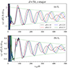 |
Fig. 5. Kink motions with (a) Sx and (b) Ax patterns in a two-elliptic-tube configuration with an x-major orientation. Plotted are the time sequences of the x speed sampled at the left tube center (vx(−d/2, 0; t), the solid curves) for a number of ratios of the semi-major to semi-minor axis (a/b) distinguished with different colors. A fitting procedure was performed for each sequence, over the duration encompassing the six extrema, starting with the one denoted by an asterisk. The best-fit damping envelope is plotted for the entire sequence, but only for a/b = 2.5 to avoid overcrowding the plots. The computations pertain to a fixed combination, |
![Mathematical equation: $ [\rho_{\mathrm{i}}/\rho_{\mathrm{e}}=3, \bar{l}=0.4, d/b=5, kb=\pi/30] $](/articles/aa/full_html/2024/06/aa49319-24/aa49319-24-eq55.gif)
The temporal attenuation of the internal flow fields means energy redistribution in ideal MHD. Let us take the case with a/b = 2.5 in Fig. 5, and note that the two tubes are actually in contact (d = 5b = 2a). Figure 6 presents the spatial distribution of the velocity fields (v = vxex + vyey, blue arrows) and the instantaneous energy density (ϵ, filled contours) for (a) the Sx motion and (b) the Ax motion at an arbitrarily chosen instant, t = 260b/vAe. A subarea of the second quadrant is singled out by each inset to emphasize the ϵ distributions in the nonuniform layers of both tubes, with the red curves delineating the layer boundaries. The white curve further indicates where the local Alfvén frequency equals the quasi-mode frequency. Figure 6 is actually taken from the animation available online. The arrows and filled contours are plotted in such a way that it makes sense to compare the v or ϵ strengths not only in one snapshot but between different instants for a given orientation. In particular, the darker a portion is, the larger the value of ϵ therein.
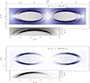 |
Fig. 6. Representative snapshots of the velocity field (the blue arrows) and energy density distribution (ϵ, filled contours) for (a) the Sx motion and (b) the Ax one in a two-elliptic-tube configuration with the x-major orientation. The inset in each panel emphasizes the distribution of ϵ in a representative nonuniform layer, whose boundaries are shown by the solid red curves. The white contour indicates where the Alfvén frequency, ωA = kvA, equals the quasi-mode frequency deduced with the fitting procedure. Both computations pertain to a fixed combination, |
![Mathematical equation: $ [\rho_{\mathrm{i}}/\rho_{\mathrm{e}}=3, a/b=2.5, \bar{l}=0.4, d/b=5, kb=\pi/30] $](/articles/aa/full_html/2024/06/aa49319-24/aa49319-24-eq56.gif)
We consider first the ambient fields of both perturbation patterns, where by “ambient” we refer to the flows some distance away from the tubes. Likewise, by “tube flow” we mean the field excluding the ambient flow, and by “internal flow” we refer specifically to the uniform portion inside either tube. For both patterns, one sees from the animation that the ambient flows tend to vary more rapidly than the internal ones. This feature is particularly clear for the Sx pattern because the ambient flows tend to be substantially stronger than the internal flows as well. Regardless, a periodogram analysis yields that the ambient flows primarily follow the external Alfvén frequency ωAe, whereas the variations of the internal flows are dominated by the lower quasi-mode frequency. That the ambient motions are not coordinated with the internal ones is a result of the form of the initial exciter given by Eq. (20). The relevant physics is actually very similar to what happens in the T08 study despite the configurational differences, the key being the y invariance of Eq. (20). It proves easier to explain this by considering a uniform equilibrium with density ρe, for which Eqs. (7)–(11) can be combined to yield a Klein-Gordon equation if the y dependence is dropped (see Eq. (1) in Terradas et al. 2005). Suppose that an individual component in Eq. (20) is applied. A dispersive fast wave then results, whereby any fluid parcel in the system eventually ends up in some oscillatory wake at the Alfvén frequency ωAe (see Fig. 1 in Terradas et al. 2005). Oscillatory wakes turn out to still exist in the ambient flow when the two elliptic tubes are introduced, and when an additional planar perturbation is implemented. It should be noted that the initial perturbations are external to our tubes. Furthermore, overall, the long-term behavior of the ambient flow actually comprises two component wakes, each being the response to the corresponding component driver. The two component wakes tend to interfere constructively (largely destructively) for the Sx (Ax) pattern, thereby explaining the strength of the ambient flow relative to the internal one.
Now, we examine the tube flows. Focusing on the blue arrows, one sees from Fig. 6 that the gross patterns for both Sx and Ax are similar to Fig. 2 in L08 despite a two-circular-tube equilibrium with a piecewise-constant profile being addressed therein. Specifically, the internal velocity field is more or less uniform, and a pair of vortical motions develop at the edge of either tube. These two features, combined with the overall symmetric properties of the internal field about x = 0, demonstrate the robustness of the classification scheme for lower-order kink motions. The primary difference with L08, on the other hand, is that the vortical motions gradually evolve from a simple dipolar behavior (see the first several instants in the animation) into multiple shearing layers (Fig. 6). This evolution is well known for kink motions in isolated tubes with either circular (e.g., Terradas et al. 2008b; Pascoe et al. 2010; Antolin et al. 2014) or elliptic cross sections (e.g., Ruderman 2003; Guo et al. 2020). What Fig. 6 demonstrates, then, is that tube interactions do not compromise the phase-mixing physics behind this evolution. That said, tube interactions do impact the detailed development of the small-scale shears, as is evidenced by the differences in the velocity fields for the two different perturbation patterns. Suppose that tube interactions are negligible. The tube flows are then expected to be identical for the Sx and Ax patterns, meaning in particular a symmetric distribution of the energy density (ϵ) with respect to the minor axis (x = −d/2 = −2.5b here). However, this expectation roughly holds only for the Sx pattern (Fig. 6a inset), whereas the left portion in the left tube is favored in the ϵ distribution for the Ax pattern (Fig. 6b inset). Besides phase mixing, a closely related aspect that is not fundamentally compromised by tube interactions is the resonant interplay between the quasi-mode and the Alfvén continuum (see Soler & Terradas 2015 and references therein for the subtle distinction between resonant absorption and phase mixing). By this, we refer to two features common to the Sx and Ax patterns, and we concentrate on the insets in the animation. Firstly, the attenuation of the internal field is accompanied by the accumulation of perturbation energies in the nonuniform layer. Secondly, this energy accumulation leads to a localized ϵ distribution, with the strongest perturbations tending to the white resonance contour as time proceeds for roughly one quasi-mode period after the rapidly varying phase. Overall, with Fig. 6 we conclude that the notions of phase mixing and resonant absorption remain applicable to kink motions in our two-elliptic-tube configuration.
Figure 7 further examines the phase-mixing process by showing the y cuts of the x speeds through the left tube center for both the (a) Sx and (b) Ax patterns. A number of instants are rather arbitrarily chosen and distinguished by different colors. The vertical dotted lines mark the borders of the nonuniform layer, where shearing motions (∂vx/∂y here) with increasingly small scales are seen to develop as time proceeds. We chose to quantify this development by relating the number of the vx extrema (Nextrm(t)) to the instantaneous phase variation accumulated over the Alfvén continuum (ϕac(t), see the discussion on Eq. (A.1)). We note that ϕac(t) = (ωAe − ωAi)t is identical for both perturbation patterns, corresponding specifically to [2.82, 4.23, 5.64] half-cycles for the examined instants. One then expects ![Mathematical equation: $ [2^{+1}_{+0}, 4^{+1}_{+0}, 5^{+1}_{+0}] $](/articles/aa/full_html/2024/06/aa49319-24/aa49319-24-eq57.gif) extrema in the vx profiles in Figs. 7a and b, which is indeed the case3. As can be readily verified, that Nextrm(t) = ⌊ϕac(t)/π⌋ at these instants actually constrains the phase, φ0, in Eq. (A.1) to a very narrow range, [qπ, (q + 0.19)π], with q = 0, 1.
extrema in the vx profiles in Figs. 7a and b, which is indeed the case3. As can be readily verified, that Nextrm(t) = ⌊ϕac(t)/π⌋ at these instants actually constrains the phase, φ0, in Eq. (A.1) to a very narrow range, [qπ, (q + 0.19)π], with q = 0, 1.
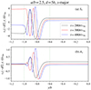 |
Fig. 7. Distributions of the x speed along the y cut through the left tube center at a number of instants as labeled. Panels a and b correspond to the Sx and Ax motions, respectively. The vertical dotted lines represent the borders of the nonuniform layer. Only the lower half (y < 0) of a y profile is displayed, the other half being symmetric with respect to y = 0. All computations were conducted for the x-major orientation with a fixed combination of physical parameters |
![Mathematical equation: $ [\rho_{\mathrm{i}}/\rho_{\mathrm{e}}=3, \bar{l}=0.4, d/b=5, kb=\pi/30] $](/articles/aa/full_html/2024/06/aa49319-24/aa49319-24-eq58.gif)
Figure 8 proceeds to examine (a) the periods, P, and (b) the damping-time-to-period ratios, τ/P, of kink quasi-modes pertaining to both the Sx (solid curves) and Ax (dashed) patterns, showing how P and τ depend on the ratio of the semi-major to semi-minor radius (a/b) for a given tube separation (d). We also examine a number of d, as is shown by the different colors. This survey adopted a fixed combination of physical parameters, ![Mathematical equation: $ [\rho_{\mathrm{i}}/\rho_{\mathrm{e}}=3, \bar{l}=0.4, kb=\pi/30] $](/articles/aa/full_html/2024/06/aa49319-24/aa49319-24-eq59.gif) . The same set of parameters was additionally adopted to evaluate P and τ/P of the kink quasi-mode for an isolated circular tube with the resistive eigenmode approach (see Sect. 3.1), the results being plotted with horizontal lines for comparison. The values for P (in units of the axial Alfvén time, Taxial = 2π/ωAe = 2L/vAe) and τ/P vary little if kb = πb/L is further reduced, meaning that little will change if one examines axial fundamentals in AR loops with much larger L/b than that adopted here. Furthermore, a/b must not exceed d/2b for a given d/b such that tube overlapping is avoided. For any given pair, [a/b, d/b], Fig. 8 indicates that the Ax motion possesses a shorter period and damps more efficiently than the Sx motion. This behavior is identical to what SL15 found for two-circular-tube configurations. The argument therein is that Ax motions are more “forced”; the two tubes move in a largely synchronous fashion for the Sx pattern, whereas the flows in between the two tubes periodically “collide” when the Ax pattern is examined. The same argument applies here, although elliptic tubes are addressed, with the insets of Fig. 6b already hinting at a more forced behavior for Ax motions. Also, similar to SL15 is that, for a given a/b, the difference between the values of P (or τ/P) for the Sx and Ax motions tends to decrease monotonically with d. This agrees with the intuitive expectation for a weaker tube interaction.
. The same set of parameters was additionally adopted to evaluate P and τ/P of the kink quasi-mode for an isolated circular tube with the resistive eigenmode approach (see Sect. 3.1), the results being plotted with horizontal lines for comparison. The values for P (in units of the axial Alfvén time, Taxial = 2π/ωAe = 2L/vAe) and τ/P vary little if kb = πb/L is further reduced, meaning that little will change if one examines axial fundamentals in AR loops with much larger L/b than that adopted here. Furthermore, a/b must not exceed d/2b for a given d/b such that tube overlapping is avoided. For any given pair, [a/b, d/b], Fig. 8 indicates that the Ax motion possesses a shorter period and damps more efficiently than the Sx motion. This behavior is identical to what SL15 found for two-circular-tube configurations. The argument therein is that Ax motions are more “forced”; the two tubes move in a largely synchronous fashion for the Sx pattern, whereas the flows in between the two tubes periodically “collide” when the Ax pattern is examined. The same argument applies here, although elliptic tubes are addressed, with the insets of Fig. 6b already hinting at a more forced behavior for Ax motions. Also, similar to SL15 is that, for a given a/b, the difference between the values of P (or τ/P) for the Sx and Ax motions tends to decrease monotonically with d. This agrees with the intuitive expectation for a weaker tube interaction.
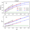 |
Fig. 8. Dependencies of (a) the quasi-mode periods (P) and (b) damping-time-to-period ratios (τ/P) on the ratio of the semi-major to semi-minor axis (a/b) for kink motions in a two-elliptic-tube configuration with the x-major orientation. The Sx and Ax patterns are distinguished by the line styles. A number of dimensionless tube separations (d/b) are examined, as is differentiated by the different colors, with d/b constrained to avoid tube overlapping. All results pertain to a fixed combination of physical parameters, |
![Mathematical equation: $ [\rho_{\mathrm{i}}/\rho_{\mathrm{e}}=3, \bar{l}=0.4, kb=\pi/30] $](/articles/aa/full_html/2024/06/aa49319-24/aa49319-24-eq60.gif)
Now, if we pay more attention to the overall tendency of P to increase monotonically with a/b for a given d/b, somewhat subtle is that tube interactions also have some effect, because increasing a/b actually brings the two tubes effectively closer, even if the distance between the tube centers is fixed. Regardless, this tube interaction only plays a minor role, given that the monotonical a/b-dependence takes place for different d and for the Sx and Ax motions alike. One may therefore expect the same a/b-dependence for isolated elliptic tubes (or equivalently d/b → ∞), in which case it is no longer necessary to distinguish between the Sx and Ax patterns. This was indeed seen in our previous IVP study (Guo et al. 2020), where we offered some heuristic argument similar to the earlier one by Ruderman (2003). For simplicity, suppose that the equilibrium configuration is transversely structured in a piecewise-constant manner. The heuristic argument then relies on the observation that the velocity normal to the tube edge plays a central role in an isolated density-enhanced tube communicating with its surroundings. Evidently, a larger a/b makes the tube edge more elongated in the x direction. Their velocities primarily x-directed, the fluid parcels in the tube interior therefore become less aware of their surroundings, meaning some enhanced effective inertia, and hence a longer period. The same argument can be invoked in this study, despite the subtlety that the fluids surrounding one tube actually embed another tube.
4.2. Sx and Ax motions for the x-minor orientation
This subsection addresses the x-minor orientation. We start with Fig. 9, where the same set of physical quantities as in Fig. 5 is employed, and the time sequences for the x speed sampled at the left tube center are presented in an identical format. A fitting procedure was once again performed for any vx sequence over the duration exactly enclosing the six extrema, starting with the one indicated by the pertinent asterisk. We take the view that the best-fit periods (P) and damping times (τ) pertain to the ideal quasi-modes supported by our two-elliptic-tube configuration.
Figure 10 focuses on the case with [a/b = 2.5, d/b = 5], following the same format as in Fig. 6 to present the velocity fields (blue arrows) and the spatial distributions of the perturbation energy density (ϵ, filled contours) at a representative instant. The tubes are quite some distance apart in this case. Also, Fig. 10 is a snapshot extracted from the animation available online. Focusing on the velocity fields, one can safely conclude from the animation that the notations of Sx and Ax make physical sense, as was proposed by L08 for two-circular-tube systems. For both perturbation patterns, the insets in the animation further indicate that the attenuation of the internal flows is accompanied by the enhancement of the perturbation energy density, ϵ, in the nonuniform layers, with the localization of ϵ strongly mediated by the Alfvén resonance. This latter point can be readily drawn from the close association of the darkest portion in either ϵ distribution with the white curve marking where the quasi-mode frequency matches the local Alfvén frequency.
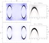 |
Fig. 10. Similar to Fig. 6 but for the x-minor orientation. The associated animation is available online. |
Figure 11 presents, in a format identical to Fig. 7, the y cuts of the x speed through the left tube center for a number of arbitrarily chosen instants. The aim is also to show the key role that phase-mixing plays for the gradual development of shearing motions with increasingly small scales in the nonuniform layers. We follow Fig. 7 to quantify this with the aid of Eq. (A.1), once again counting the instantaneous number, Nextrm(t), of the vx extrema. The pertinent instantaneous phase variations (ϕac(t)), on the other hand, are the same as in Fig. 7 and read as [2.82, 4.23, 5.64]π for the examined instants. However, somewhat different is that the relevant values of Nextrm may now deviate from ⌊ϕac/π⌋, attaining specifically [3, 4, 5]. This deviation is readily attributable to the phase, φ0, in Eq. (A.1). Conversely, this set of deviations can be readily verified to constrain φ0 to a rather narrow range of [(q + 0.19)π, (q + 0.37)π], with q = 0, 1.
Figure 12 moves on to survey (a) the quasi-mode periods, P, and (b) damping-time-to-period ratios, τ/P, of a substantial range of combinations, [a/b, d/b]. This figure is identical in format to Fig. 8. The values examined for the tube separation, d, consistently avoid tube overlapping, and hence there is no need to constrain the ratio of the semi-major to semi-minor axis (a/b) for a given d/b. Examining Fig. 12a first, one sees the expected monotonic behavior for the differences between the Sx and Ax periods decreasing with d/b for a given a/b. For a given separation, d/b, one further sees that the values of P tend to decrease monotonically with a/b for the Sx and Ax motions alike. However, it is possible that tube interactions remain partly responsible for this a/b-dependence, because the area between the two tubes actually broadens with a/b even if d/b is fixed. This tube-interaction effect can hardly be dismissed, given that the Sx and Ax values deviate more strongly when a/b increases for a given d/b. Having said that, it remains possible to partly explain the monotonic a/b-dependence of P by invoking the inertia arguments initially offered for isolated density-enhanced elliptic tubes. It should be noted that the tube edges are now more elongated in the y direction, whereas the fluids parcels in either tube interior still oscillate primarily in the x direction. It therefore holds that an increase in a/b makes the internal fluid parcels better aware of the external medium, meaning some reduced effective inertia, and hence a shorter period.
We turn now to Fig. 12b where the damping-time-to-period ratios (τ/P) are examined. Two features arise when a/b ≲ 1.5, one being that Ax motions attenuate more efficiently than Sx ones, the other being that the differences between the Sx and Ax values tend to decrease with tube separation. These features resemble what happens for two-circular-tube systems, and are expected because the cross-sectional shapes are near-circular. However, the behavior of τ/P at larger a/b is considerably more complicated than in Fig. 8b, where the x-major orientation is addressed. By “complicated”, we specifically refer to the nonmonotoic d/b-dependence of τ/P for either perturbation pattern. If we take the case with a/b = 2.5; when d/b increases, one sees an increase followed by some decrease in τ/P for the Sx motion, whereas τ/P tends to decrease for the Ax motion. This latter simplicity is only apparent because τ/P is bound to increase with d/b again such that the Ax values eventually join their Sx counterparts when the tubes are sufficiently separated. We have verified that the somehow involved behavior of τ/P is not of numerical origin (see Sect. 3). Furthermore, it matters little to how to choose the segment of a vx sequence for fitting, provided that this segment starts sufficiently later than the rapidly varying phase (see Fig. 9). The most likely reason, then, is that the perturbations in between the two tubes depend on a/b and d/b in an intricate fashion, and hence an intricate dependence on a/b and d/b of the efficiency of tube interactions. Regardless, the reason behind the d/b-dependence of τ/P is also behind, say, the nonmonotonic a/b-dependence of τ/P for Ax motions for a given d/b (see the dashed curves), and the occasional tendency of Sx motions to damp more efficiently (compare the solid and dashed black curves).
5. Implications for coronal seismology
This section discusses some seismological implications of our study. Only axial fundamentals were considered. We restricted ourselves to the inference of the axial Alfvén time (Taxial = 2L/vAe) and the dimensionless nonuniform layer width ( ). We further assumed that neighboring elliptic tubes are imaged in, say, the EUV when the line of sight lies in the tube plane (see Fig. 1a), meaning that the tubes may be readily mistaken for circular ones.
We start with Fig. 8, where our x-major computations are summarized, and consider only the Sx motion for [a/b = 2.5, d/b = 5]. We assumed that the relevant oscillating tubes possess the “true” dimensionless values, ![Mathematical equation: $ [\rho_{\mathrm{i}}/\rho_{\mathrm{e}}=3, \bar{l}=0.4] $](/articles/aa/full_html/2024/06/aa49319-24/aa49319-24-eq62.gif) (L/b is immaterial when sufficiently large). Pobs and (τ/P)obs are the measured values of the period and damping-time-to-period ratio, and we took (τ/P)obs = 6.39 to comply with Fig. 8. In this way, one deduces a “true” value of Pobs/1.6 for Taxial, which is recalled to be dimensional. Now, supposing that the density contrast is measured to be ρi/ρe = 3, we follow the customary practice to infer Taxial and
(L/b is immaterial when sufficiently large). Pobs and (τ/P)obs are the measured values of the period and damping-time-to-period ratio, and we took (τ/P)obs = 6.39 to comply with Fig. 8. In this way, one deduces a “true” value of Pobs/1.6 for Taxial, which is recalled to be dimensional. Now, supposing that the density contrast is measured to be ρi/ρe = 3, we follow the customary practice to infer Taxial and  by seeing the Sx motion as a kink quasi-mode in an isolated circular tube. It matters little whether one assigns a or b to the tube radius. The dimensionless quasi-mode period, P/Taxial, depends essentially only on ρi/ρe, always attaining ∼1.42 when
  (see the horizontal green line in Fig. 8a; see also Fig. 2b). One therefore deduces a value of Pobs/1.42 for Taxial, which differs from the true value by ∼13%. However, it is considerably more problematic when (τ/P)obs is invoked to infer
  . Employing the resistive eigenmode approach, we find that a (τ/P)obs = 6.39 results in a
  , which underestimates the true value by ∼55%. One may argue that this difference is not that significant; after all, the customary seismological practice yields the correct qualitative picture that the oscillating tube possesses a thin boundary. Our point, however, is that care needs to be exercised when (τ/P)obs is put to quantitative use, with the uncertainties in the deduced dimensionless layer width,
  , readily exceeding ∼50% if one neglects the combined effect of tube cross-sectional shapes and tube interactions.
Now, we move on to Fig. 12, where our x-minor computations are summarized. We assessed what uncertainties the customary practice may introduce to the axial Alfvén time, Taxial = 2L/vAe, and dimensionless layer width,  , by neglecting the joint effects of cross-sectional shapes and tube interactions. The procedure is identical to what we performed for the x-major orientation; we accordingly chose the Ax values of [a/b = 2.5, d/b = 3], given that they deviate the most from the horizontal lines. Considering the period first, one infers a true value of Taxial = Pobs/1.13 with Fig. 12a, whereas the customary practice remains to yield a Taxial ≈ Pobs/1.42 or, equivalently, some underestimation by ∼20%. This uncertainty in Taxial is larger than that for the x-major orientation. Now, taking (τ/P)obs = 3.44 from Fig. 12b as measured, one deduces with the customary practice a dimensionless layer width of
  or some underestimation of the true value (
 ) by ∼38%. Although somewhat smaller than in the x-major case, this uncertainty remains substantial enough to corroborate our claim that the inhomogeneity scales deduced in the customary fashion need to be treated with caution.
6. Summary
With coordinated transverse displacements in neighboring AR loops in mind, we have addressed damped kink motions in straight equilibria where two identical parallel density-enhanced tubes with elliptic cross sections (elliptic tubes) are embedded in an ambient corona. Linear, ideal, pressureless MHD was adopted throughout. We concentrated on axially standing motions, formulating the ensuing 2D IVP in the plane transverse to the equilibrium magnetic field. We identified the direction connecting the tube centers as horizontal, discriminating between two tube orientations where either the major (dubbed “x-major”) or minor (“x-minor”) axis is horizontally placed. The system evolution was initiated with external velocity drivers, implemented in such a way that the internal flow fields are primarily horizontal and are either symmetric (Sx) or antisymmetric (Ax) with respect to the vertical axis about which our equilibrium configuration is symmetric. The temporal evolution of the velocity perturbations at tube centers was of particular interest, allowing us to identify the quasi-mode stage as where the monochromatic time sequence follows an exponentially damped envelope. We paid special attention to how the quasi-mode periods and damping times depend on the tube separation and the cross-sectional aspect ratio, thereby addressing the impact on the dispersive properties of damped kink motions from the joint effects of tube interactions and cross-sectional shapes.
Our numerical findings are summarized as follows. When two-circular-tube equilibria are examined as a special case, the quasi-mode periods and damping times found with our IVP approach are consistent with the modal analysis by Soler & Luna (2015), thereby independently justifying both the analytical T-matrix approach and the numerical results therein. We further find that the notions of resonant absorption and phase mixing are not undermined when elliptic cross sections are allowed for. Specifically, the nonuniform layers around tube boundaries feature both the development of velocity shears with increasingly small scales and energy accumulation around where the local Alfvén frequency matches the quasi-mode frequency. The Ax motions are found to possess shorter periods and to damp more rapidly than the Sx motions of the x-major orientation, in which case the periods and damping times for both perturbation patterns tend to increase with the major-to-minor-axis ratio. When the x-minor orientation is addressed, the Ax motions continue to oscillate more rapidly than the Sx ones. However, the periods for both patterns tend to decrease monotonically with the major-to-minor-axis ratio. Somewhat subtle are the joint effects of tube interactions and cross-sectional shapes on the damping times, which may depend non-monotonically on the tube separation or the major-to-minor-axis ratio. Furthermore, the Ax motions may occasionally damp less efficiently. Neglecting these joint effects may introduce some uncertainty of ∼20% (∼50%) to the axial Alfvén time (the inhomogeneity lengthscale) deduced with the period (damping time). Consequently, care may need to be exercised when the damping times of kink motions are put to standard seismological practice built on wave theories for isolated circular tubes.
Some further remarks seem necessary before closing. Firstly, we note that our IVP approach is not restricted to two-tube systems but capable of handling rather generic 2D inhomogeneities. In particular, axially standing motions may be examined for straight configurations comprising multiple tubular structures with arbitrary cross sections. Collective motions in multiple neighboring resolved loops will then be better understood, together with the motions in those apparently isolated loops that actually involve a multitude of unresolved strands (see e.g., Sect. 4.2 of the review by Reale 2014 for more on this multi-stranded nature of AR loops). Secondly, that kink motions are resonantly absorbed for configurations with continuous transverse structuring was actually widely expected (e.g., the review by Goossens et al. 2011). However, what has gone largely unnoticed is that the decayless regime was also observed for coordinated kink motions in adjacent AR loops (Wang et al. 2012). If we accept that the transverse structuring is likely to be continuous in the relevant configurations, it then becomes necessary to address what counteracts the ensuing resonant damping, thereby bringing the understanding of decayless kink motions in multi-tube systems closer to the level of sophistication reached for the decayless regime in isolated tubes (e.g., Nakariakov et al. 2016; Guo et al. 2019b; Ruderman et al. 2021). Thirdly, coordinated motions in multiple tubular structures were identified not only in AR loops but also in, say, groups of prominence threads (see e.g., Arregui et al. 2018, for a review). To our knowledge, so far the only theoretical investigation in the prominence context was the one by Soler et al. (2009) with the T-matrix formalism. An IVP perspective is expected to be as fruitful, provided that one further accounts for, say, the effects associated with partial ionization (e.g., the review by Ballester et al. 2018).
Movies
Movie 1 associated with Fig. 6 Access Supplementary Material
Movie 2 associated with Fig. 10 Access Supplementary Material
A uniform resistivity η is employed for simplicity, the associated magnetic Reynolds number Rm := μ0ℛvAi/η = 105. We have verified that further increasing Rm does not introduce any discernible difference to the oscillation frequencies and damping rates. These η-independent values are well known to be physically connected to ideal quasi-modes (e.g., Poedts & Kerner 1991; Terradas et al. 2006; Soler et al. 2013).
Some discrepancy exists in the literature regarding the damping of lower-order kink motions when the tubes are in contact. The T-matrix results by SL15 indicate that these motions remain damped (see Fig. 2 therein), whereas damping was found to disappear in the modal studies formulated in bicylindrical coordinates (Robertson & Ruderman 2011; Gijsen & Van Doorsselaere 2014). Our IVP study supports the SL15 conclusion. The use of a bicylindrical coordinate system was recognized by the referenced studies to be physically problematic for small tube separations.
The velocity shears are prone to the Kelvin-Helmholtz instability (KHi), as was first theoretically recognized in the wave context by Heyvaerts & Priest (1983) and Browning & Priest (1984). Further nonlinear simulations have demonstrated that the KHi may arise in the early stage of the evolution of kink motions for isolated tubes (e.g., Terradas et al. 2008b; Antolin et al. 2015; Shi et al. 2021) and multi-tube setups alike (e.g., Magyar & Van Doorsselaere 2016; Guo et al. 2019a). The applicability of such linear results as presented here may therefore need to be assessed on a case-by-case basis when real data are analyzed (see Sect. 10 of the review by Nakariakov et al. 2021, for more on the nonlinear aspects).
Acknowledgments
This research was supported by the National Natural Science Foundation of China (41974200, 12273019, 12373055, 12203030, and 42230203). We gratefully acknowledge ISSI-BJ for supporting the international team “Magnetohydrodynamic wavetrains as a tool for probing the solar corona”, and ISSI-Bern for supporting the international team “Magnetohydrodynamic Surface Waves at Earth’s Magnetosphere and Beyond”.
References
- Aldhafeeri, A. A., Verth, G., Brevis, W., et al. 2021, ApJ, 912, 50 [CrossRef] [Google Scholar]
- Anderson, J. D. 1995, Computational Fluid Dynamics: The Basics with Applications (New York: McGraw-Hill, Inc.) [Google Scholar]
- Anfinogentov, S. A., & Nakariakov, V. M. 2019, ApJ, 884, L40 [CrossRef] [Google Scholar]
- Anfinogentov, S., Nisticò, G., & Nakariakov, V. M. 2013, A&A, 560, A107 [NASA ADS] [CrossRef] [EDP Sciences] [Google Scholar]
- Anfinogentov, S. A., Nakariakov, V. M., & Nisticò, G. 2015, A&A, 583, A136 [NASA ADS] [CrossRef] [EDP Sciences] [Google Scholar]
- Antolin, P., Yokoyama, T., & Van Doorsselaere, T. 2014, ApJ, 787, L22 [Google Scholar]
- Antolin, P., Okamoto, T. J., De Pontieu, B., et al. 2015, ApJ, 809, 72 [Google Scholar]
- Arregui, I. 2022, Front. Astron. Space Sci., 9, 826947 [NASA ADS] [CrossRef] [Google Scholar]
- Arregui, I., & Asensio Ramos, A. 2011, ApJ, 740, 44 [NASA ADS] [CrossRef] [Google Scholar]
- Arregui, I., Soler, R., & Asensio Ramos, A. 2015, ApJ, 811, 104 [CrossRef] [Google Scholar]
- Arregui, I., Oliver, R., & Ballester, J. L. 2018, Liv. Rev. Sol. Phys., 15, 3 [Google Scholar]
- Aschwanden, M. J., & Schrijver, C. J. 2011, ApJ, 736, 102 [NASA ADS] [CrossRef] [Google Scholar]
- Aschwanden, M. J., Fletcher, L., Schrijver, C. J., & Alexander, D. 1999, ApJ, 520, 880 [Google Scholar]
- Aschwanden, M. J., Nightingale, R. W., Andries, J., Goossens, M., & Van Doorsselaere, T. 2003, ApJ, 598, 1375 [NASA ADS] [CrossRef] [Google Scholar]
- Aschwanden, M. J., Nakariakov, V. M., & Melnikov, V. F. 2004, ApJ, 600, 458 [NASA ADS] [CrossRef] [Google Scholar]
- Ballester, J. L., Alexeev, I., Collados, M., et al. 2018, Space Sci. Rev., 214, 58 [Google Scholar]
- Bogdan, T. J., & Zweibel, E. G. 1985, ApJ, 298, 867 [NASA ADS] [CrossRef] [Google Scholar]
- Bogdan, T. J., & Zweibel, E. G. 1987, ApJ, 312, 444 [CrossRef] [Google Scholar]
- Browning, P. K., & Priest, E. R. 1984, A&A, 131, 283 [NASA ADS] [Google Scholar]
- Cally, P. S. 1986, Sol. Phys., 103, 277 [Google Scholar]
- Chen, S.-X., Li, B., Van Doorsselaere, T., et al. 2021, ApJ, 908, 230 [NASA ADS] [CrossRef] [Google Scholar]
- De Moortel, I., & Nakariakov, V. M. 2012, Philos. Trans. R. Soc. London Ser. A, 370, 3193 [NASA ADS] [Google Scholar]
- Edwin, P. M., & Roberts, B. 1983, Sol. Phys., 88, 179 [Google Scholar]
- Erdélyi, R., & Morton, R. J. 2009, A&A, 494, 295 [NASA ADS] [CrossRef] [EDP Sciences] [Google Scholar]
- Erdélyi, R., & Taroyan, Y. 2008, A&A, 489, L49 [NASA ADS] [CrossRef] [EDP Sciences] [Google Scholar]
- Gijsen, S. E., & Van Doorsselaere, T. 2014, A&A, 562, A38 [NASA ADS] [CrossRef] [EDP Sciences] [Google Scholar]
- Goddard, C. R., Nisticò, G., Nakariakov, V. M., & Zimovets, I. V. 2016, A&A, 585, A137 [NASA ADS] [CrossRef] [EDP Sciences] [Google Scholar]
- Goedbloed, H., Keppens, R., & Poedts, S. 2019, Magnetohydrodynamics of Laboratory and Astrophysical Plasmas (Cambridge: Cambridge University Press) [Google Scholar]
- Goossens, M., Hollweg, J. V., & Sakurai, T. 1992, Sol. Phys., 138, 233 [Google Scholar]
- Goossens, M., Andries, J., & Aschwanden, M. J. 2002, A&A, 394, L39 [NASA ADS] [CrossRef] [EDP Sciences] [Google Scholar]
- Goossens, M., Arregui, I., Ballester, J. L., & Wang, T. J. 2008, A&A, 484, 851 [NASA ADS] [CrossRef] [EDP Sciences] [Google Scholar]
- Goossens, M., Erdélyi, R., & Ruderman, M. S. 2011, Space Sci. Rev., 158, 289 [Google Scholar]
- Guo, M., Van Doorsselaere, T., Karampelas, K., & Li, B. 2019a, ApJ, 883, 20 [NASA ADS] [CrossRef] [Google Scholar]
- Guo, M., Van Doorsselaere, T., Karampelas, K., et al. 2019b, ApJ, 870, 55 [Google Scholar]
- Guo, M., Li, B., & Van Doorsselaere, T. 2020, ApJ, 904, 116 [Google Scholar]
- Heyvaerts, J., & Priest, E. R. 1983, A&A, 117, 220 [NASA ADS] [Google Scholar]
- Hong, H. 1996, Appl. Math. Lett., 9, 99 [Google Scholar]
- Jardin, S. 2010, Computational Methods in Plasma Physics, Chapman& Hall/CRC Computational Science (CRC Press) [Google Scholar]
- Keppens, R., Bogdan, T. J., & Goossens, M. 1994, ApJ, 436, 372 [NASA ADS] [CrossRef] [Google Scholar]
- Klimchuk, J. A., & DeForest, C. E. 2020, ApJ, 900, 167 [NASA ADS] [CrossRef] [Google Scholar]
- Klimchuk, J. A., Lemen, J. R., Feldman, U., Tsuneta, S., & Uchida, Y. 1992, PASJ, 44, L181 [NASA ADS] [CrossRef] [Google Scholar]
- Kucera, T. A., Young, P. R., Klimchuk, J. A., & DeForest, C. E. 2019, ApJ, 885, 7 [NASA ADS] [CrossRef] [Google Scholar]
- Li, D., & Long, D. M. 2023, ApJ, 944, 8 [NASA ADS] [CrossRef] [Google Scholar]
- Li, B., Antolin, P., Guo, M. Z., et al. 2020, Space Sci. Rev., 216, 136 [NASA ADS] [CrossRef] [Google Scholar]
- Li, B., Chen, S.-X., & Li, A.-L. 2022, ApJ, 928, 33 [NASA ADS] [CrossRef] [Google Scholar]
- Lin, Y., Engvold, O. R., & Wiik, J. E. 2003, Sol. Phys., 216, 109 [NASA ADS] [CrossRef] [Google Scholar]
- Luna, M., Terradas, J., Oliver, R., & Ballester, J. L. 2008, ApJ, 676, 717 [NASA ADS] [CrossRef] [Google Scholar]
- Luna, M., Terradas, J., Oliver, R., & Ballester, J. L. 2009, ApJ, 692, 1582 [NASA ADS] [CrossRef] [Google Scholar]
- Luna, M., Terradas, J., Oliver, R., & Ballester, J. L. 2010, ApJ, 716, 1371 [NASA ADS] [CrossRef] [Google Scholar]
- Luna, M., Oliver, R., Antolin, P., & Arregui, I. 2019, A&A, 629, A20 [NASA ADS] [CrossRef] [EDP Sciences] [Google Scholar]
- MacCormack, R. W. 1969, AIAA Paper, 69, 354 [Google Scholar]
- Magyar, N., & Van Doorsselaere, T. 2016, ApJ, 823, 82 [CrossRef] [Google Scholar]
- Malanushenko, A., & Schrijver, C. J. 2013, ApJ, 775, 120 [NASA ADS] [CrossRef] [Google Scholar]
- Mann, I. R., Wright, A. N., & Cally, P. S. 1995, J. Geophys. Res., 100, 19441 [Google Scholar]
- McCarthy, M. I., Longcope, D. W., & Malanushenko, A. 2021, ApJ, 913, 56 [NASA ADS] [CrossRef] [Google Scholar]
- Morton, R. J., & Ruderman, M. S. 2011, A&A, 527, A53 [NASA ADS] [CrossRef] [EDP Sciences] [Google Scholar]
- Nakariakov, V. M., & Kolotkov, D. Y. 2020, ARA&A, 58, 441 [Google Scholar]
- Nakariakov, V. M., & Ofman, L. 2001, A&A, 372, L53 [NASA ADS] [CrossRef] [EDP Sciences] [Google Scholar]
- Nakariakov, V. M., & Verwichte, E. 2005, Liv. Rev. Sol. Phys., 2, 3 [Google Scholar]
- Nakariakov, V. M., Ofman, L., Deluca, E. E., Roberts, B., & Davila, J. M. 1999, Science, 285, 862 [Google Scholar]
- Nakariakov, V. M., Anfinogentov, S. A., Nisticò, G., & Lee, D. H. 2016, A&A, 591, L5 [NASA ADS] [CrossRef] [EDP Sciences] [Google Scholar]
- Nakariakov, V. M., Anfinogentov, S. A., Antolin, P., et al. 2021, Space Sci. Rev., 217, 73 [NASA ADS] [CrossRef] [Google Scholar]
- Nechaeva, A., Zimovets, I. V., Nakariakov, V. M., & Goddard, C. R. 2019, ApJS, 241, 31 [NASA ADS] [CrossRef] [Google Scholar]
- Nisticò, G., Nakariakov, V. M., & Verwichte, E. 2013, A&A, 552, A57 [NASA ADS] [CrossRef] [EDP Sciences] [Google Scholar]
- Ofman, L. 2009, ApJ, 694, 502 [NASA ADS] [CrossRef] [Google Scholar]
- Ofman, L., & Wang, T. J. 2008, A&A, 482, L9 [NASA ADS] [CrossRef] [EDP Sciences] [Google Scholar]
- Okamoto, T. J., Tsuneta, S., Berger, T. E., et al. 2007, Science, 318, 1577 [Google Scholar]
- Pascoe, D. J., Wright, A. N., & De Moortel, I. 2010, ApJ, 711, 990 [Google Scholar]
- Petrova, E., Magyar, N., Van Doorsselaere, T., & Berghmans, D. 2023, ApJ, 946, 36 [CrossRef] [Google Scholar]
- Poedts, S., & Kerner, W. 1991, Phys. Rev. Lett., 66, 2871 [NASA ADS] [CrossRef] [Google Scholar]
- Reale, F. 2014, Liv. Rev. Sol. Phys., 11, 4 [Google Scholar]
- Roberts, B. 2019, MHD Waves in the Solar Atmosphere (Cambridge: Cambridge University Press) [Google Scholar]
- Robertson, D., & Ruderman, M. S. 2011, A&A, 525, A4 [NASA ADS] [CrossRef] [EDP Sciences] [Google Scholar]
- Robertson, D., Ruderman, M. S., & Taroyan, Y. 2010, A&A, 515, A33 [NASA ADS] [CrossRef] [EDP Sciences] [Google Scholar]
- Ruderman, M. S. 2003, A&A, 409, 287 [NASA ADS] [CrossRef] [EDP Sciences] [Google Scholar]
- Ruderman, M. S., & Petrukhin, N. S. 2023, MNRAS, 523, 2074 [NASA ADS] [CrossRef] [Google Scholar]
- Ruderman, M. S., & Roberts, B. 2002, ApJ, 577, 475 [Google Scholar]
- Ruderman, M. S., Petrukhin, N. S., & Pelinovsky, E. 2021, Sol. Phys., 296, 124 [NASA ADS] [CrossRef] [Google Scholar]
- Sakurai, T., Goossens, M., & Hollweg, J. V. 1991, Sol. Phys., 133, 227 [Google Scholar]
- Schrijver, C. J. 2007, ApJ, 662, L119 [NASA ADS] [CrossRef] [Google Scholar]
- Schrijver, C. J., & Brown, D. S. 2000, ApJ, 537, L69 [NASA ADS] [CrossRef] [Google Scholar]
- Schrijver, C. J., Title, A. M., Berger, T. E., et al. 1999, Sol. Phys., 187, 261 [NASA ADS] [CrossRef] [Google Scholar]
- Schrijver, C. J., Aschwanden, M. J., & Title, A. M. 2002, Sol. Phys., 206, 69 [Google Scholar]
- Sescu, A. 2015, Adv. Differ. Equ., 2015, 1 [CrossRef] [Google Scholar]
- Sewell, G. 1988, The Numerical Solution of Ordinary and Partial Differential Equations (San Diego: Academic Press) [Google Scholar]
- Shi, M., Li, B., & Yuan, S. 2024, A&A, 684, A154 [NASA ADS] [CrossRef] [EDP Sciences] [Google Scholar]
- Shi, M., Van Doorsselaere, T., Guo, M., et al. 2021, ApJ, 908, 233 [Google Scholar]
- Soler, R., & Luna, M. 2015, A&A, 582, A120 [NASA ADS] [CrossRef] [EDP Sciences] [Google Scholar]
- Soler, R., & Terradas, J. 2015, ApJ, 803, 43 [Google Scholar]
- Soler, R., Oliver, R., & Ballester, J. L. 2009, ApJ, 693, 1601 [NASA ADS] [CrossRef] [Google Scholar]
- Soler, R., Goossens, M., Terradas, J., & Oliver, R. 2013, ApJ, 777, 158 [Google Scholar]
- Soler, R., Goossens, M., Terradas, J., & Oliver, R. 2014, ApJ, 781, 111 [NASA ADS] [CrossRef] [Google Scholar]
- Terradas, J., Oliver, R., & Ballester, J. L. 2005, ApJ, 618, L149 [NASA ADS] [CrossRef] [Google Scholar]
- Terradas, J., Oliver, R., & Ballester, J. L. 2006, ApJ, 642, 533 [Google Scholar]
- Terradas, J., Arregui, I., Oliver, R., et al. 2008a, ApJ, 679, 1611 [NASA ADS] [CrossRef] [Google Scholar]
- Terradas, J., Andries, J., Goossens, M., et al. 2008b, ApJ, 687, L115 [Google Scholar]
- Tian, H., McIntosh, S. W., Wang, T., et al. 2012, ApJ, 759, 144 [Google Scholar]
- Tirry, W. J., & Goossens, M. 1996, ApJ, 471, 501 [Google Scholar]
- Van Doorsselaere, T., Andries, J., Poedts, S., & Goossens, M. 2004, ApJ, 606, 1223 [Google Scholar]
- Van Doorsselaere, T., Nakariakov, V. M., Young, P. R., & Verwichte, E. 2008a, A&A, 487, L17 [NASA ADS] [CrossRef] [EDP Sciences] [Google Scholar]
- Van Doorsselaere, T., Ruderman, M. S., & Robertson, D. 2008b, A&A, 485, 849 [NASA ADS] [CrossRef] [EDP Sciences] [Google Scholar]
- Verwichte, E., Nakariakov, V. M., Ofman, L., & Deluca, E. E. 2004, Sol. Phys., 223, 77 [Google Scholar]
- Verwichte, E., Aschwanden, M. J., Van Doorsselaere, T., Foullon, C., & Nakariakov, V. M. 2009, ApJ, 698, 397 [NASA ADS] [CrossRef] [Google Scholar]
- Verwichte, E., Van Doorsselaere, T., White, R. S., & Antolin, P. 2013, A&A, 552, A138 [NASA ADS] [CrossRef] [EDP Sciences] [Google Scholar]
- Wang, H., & Sakurai, T. 1998, PASJ, 50, 111 [NASA ADS] [CrossRef] [Google Scholar]
- Wang, T. J., Solanki, S. K., & Selwa, M. 2008, A&A, 489, 1307 [NASA ADS] [CrossRef] [EDP Sciences] [Google Scholar]
- Wang, T., Ofman, L., Davila, J. M., & Su, Y. 2012, ApJ, 751, L27 [Google Scholar]
- Watko, J. A., & Klimchuk, J. A. 2000, Sol. Phys., 193, 77 [NASA ADS] [CrossRef] [Google Scholar]
- White, R. S., & Verwichte, E. 2012, A&A, 537, A49 [NASA ADS] [CrossRef] [EDP Sciences] [Google Scholar]
- White, R. S., Verwichte, E., & Foullon, C. 2013, ApJ, 774, 104 [NASA ADS] [CrossRef] [Google Scholar]
- Williams, T., Walsh, R. W., & Morgan, H. 2021, ApJ, 919, 47 [NASA ADS] [CrossRef] [Google Scholar]
- Yi, Z., Engvold, O., & Keil, S. L. 1991, Sol. Phys., 132, 63 [NASA ADS] [CrossRef] [Google Scholar]
- Yu, H., Li, B., Chen, S., & Guo, M. 2021, Sol. Phys., 296, 95 [NASA ADS] [CrossRef] [Google Scholar]
- Zajtsev, V. V., & Stepanov, A. V. 1975, Issledovaniia Geomagnetizmu Aeronomii i Fizike Solntsa, 37, 3 [NASA ADS] [Google Scholar]
- Zhong, S., Nakariakov, V. M., Kolotkov, D. Y., Verbeeck, C., & Berghmans, D. 2022, MNRAS, 516, 5989 [NASA ADS] [CrossRef] [Google Scholar]
- Zhong, S., Nakariakov, V. M., Kolotkov, D. Y., et al. 2023, Nat. Commun., 14, 5298 [NASA ADS] [CrossRef] [Google Scholar]
- Zimovets, I. V., & Nakariakov, V. M. 2015, A&A, 577, A4 [NASA ADS] [CrossRef] [EDP Sciences] [Google Scholar]
Appendix A: Subtleties with domain size and grid spacing
This appendix examines the influences that the numerical grid setup may have on our time-dependent solutions, taking two-circular-tube computations as examples. Our ![Mathematical equation: $ [b, \bar{l}] $](/articles/aa/full_html/2024/06/aa49319-24/aa49319-24-eq71.gif) notations are used together with the RR02 convention, [ℛ, ℓ]. It suffices to address only the Sx pattern for a fixed combination of physical parameters, [ρi/ρe = 5, ℓ/ℛ = 0.4, d/ℛ = 2.5, kb = π/30].
notations are used together with the RR02 convention, [ℛ, ℓ]. It suffices to address only the Sx pattern for a fixed combination of physical parameters, [ρi/ρe = 5, ℓ/ℛ = 0.4, d/ℛ = 2.5, kb = π/30].
We start with Fig. A.1 by displaying the temporal evolution of the x speed at the left tube center (vx(−d/2, 0; t), solid curves) for a number of domain sizes, [xM, yM], that are distinguished with different colors. The best-fit damping envelopes are further plotted by the dashed curves for reference. All computations pertain to a fixed grid spacing, Δ = 0.01b, which is recalled to be different from the reference value in Table 1. Some differences are seen among the solid curves, the most prominent one being that the monochromatic cycles in the vx signal are slightly delayed when the domain size increases. We find that this domain size effect arises because the zero-gradient boundary condition is not fully transparent to impinging motions initiated with the pair of planar perturbations given by Eq. (20). Some weakly reflected disturbances reach and interact with the composite structure, resulting in it taking longer for the internal flow fields to settle on a regular pattern for a larger domain. That the domain size effect is primarily attributed to the form of the initial perturbation is further corroborated by an additional series of computations where we multiply each exponential term in Eq. (20) by a factor, exp(−y2/b2). The dependence on the domain size is then found to disappear in the time-dependent solutions responding to this localized perturbation. A monochromatic pattern remains clearly visible after some transitory phase, the period being nearly identical to what we find when Eq. (20) is employed. However, the damping envelope deviates considerably from an exponential one, making it difficult to examine ideal quasi-modes from an IVP perspective. The reasons for us to stick to Eq. (20) are twofold. Firstly, what drives the internal field toward a quasi-mode behavior is beyond our scope. Rather, we content ourselves with deriving the relevant periods and damping times. Secondly, varying the domain size does not influence the best-fit period (Pfit) and only marginally impacts the best-fit damping time (τfit). In fact, Pfit always evaluates to ∼112.5b/vAe for the examined domains. The value of τfitvAe/b, on the other hand, changes from 320.1 for [xM = 12b, yM = 10b] only modestly to 313.3 for [xM = 18b, yM = 15b]. An even weaker variation is found when the domain is further extended to [xM = 24b, yM = 20b], in which case τfitvAe/b attains 314.3.
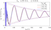 |
Fig. A.1. Temporal profiles of the x speed sampled at the left tube center (vx(−d/2, 0; t), the solid curves) for a number of domain sizes as labeled. Overplotted by the dashed curves are the best-fit damping envelopes. All computations pertain to the Sx motion for a fixed combination of physical parameters, [ρi/ρe = 5, ℓ/ℛ = 0.4, d/ℛ = 2.5, kb = π/30]. The grid spacing is fixed at Δ = 0.01b. |
One may ask why we chose a spacing, Δ = 0.01b, different from the reference value (Δ = 0.005b) when examining the domain size effect. The answer is that the specific values of Δ do not impact the vx(−d/2, 0; t) sequences for a given domain size if Δ is sufficiently small. By “sufficiently” we mean some criterion related to the pair of equilibrium quantities, ![Mathematical equation: $ [\rho_{\mathrm{i}}/\rho_{\mathrm{e}}, \bar{l}] $](/articles/aa/full_html/2024/06/aa49319-24/aa49319-24-eq72.gif) (see Sect. 2.4). We reach this statement by varying only Δ for a substantial fraction of the computations in Fig. 4. If we consider only those with the reference domain size, Figure A.2 offers a representative case, with ℓ/ℛ = 0.4, by discriminating the vx(−d/2, 0; t) sequences for different Δ with different line styles. Relative to the computation with the reference Δ (the dashed red curve), no difference can be discerned when the spacing is halved (dash-dotted blue line) or doubled (dotted black line). The reference Δ is therefore overly demanding of computational resources for ℓ/ℛ = 0.4, and the same can be said even for the most stringent case where ℓ/ℛ = 0.2, provided that only vx(−d/2, 0; t) is of interest. That said, varying Δ necessarily entails differences in other aspects of the flow fields. We illustrate this point by fixing ℓ/ℛ again at 0.4 and implementing the reference domain size.
(see Sect. 2.4). We reach this statement by varying only Δ for a substantial fraction of the computations in Fig. 4. If we consider only those with the reference domain size, Figure A.2 offers a representative case, with ℓ/ℛ = 0.4, by discriminating the vx(−d/2, 0; t) sequences for different Δ with different line styles. Relative to the computation with the reference Δ (the dashed red curve), no difference can be discerned when the spacing is halved (dash-dotted blue line) or doubled (dotted black line). The reference Δ is therefore overly demanding of computational resources for ℓ/ℛ = 0.4, and the same can be said even for the most stringent case where ℓ/ℛ = 0.2, provided that only vx(−d/2, 0; t) is of interest. That said, varying Δ necessarily entails differences in other aspects of the flow fields. We illustrate this point by fixing ℓ/ℛ again at 0.4 and implementing the reference domain size.
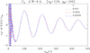 |
Fig. A.2. Temporal profiles of the x speed sampled at the left tube center for a number of grid spacings as labeled. All computations pertain to the Sx motion for a fixed combination of physical parameters, [ρi/ρe = 5, ℓ/ℛ = 0.4, d/ℛ = 2.5, kb = π/30]. The computational domain size is fixed at [xM = 12b, yM = 10b]. |
Figure A.3 presents the spatial profiles of the x speed along the y cut through the left tube center at t = 340b/vAe. This instant was chosen rather arbitrarily to be marginally inside the interval where our fitting procedure was performed. A cut through a tube center, on the other hand, was chosen to ease the description of some key dynamics. A number of grid spacings were implemented and are distinguished with different colors. Only the lower half (y ≤ 0) of a y profile is displayed because the other half is symmetric with respect to y = 0. The vertical dash-dotted lines represent the borders of the nonuniform layer. Focusing for now on this layer, one sees a series of ripples in all computations. The most prominent effect associated with Δ is that the ripples are better resolved when the numerical grid gets finer, with the computed magnitudes of the local extrema being larger. Physically speaking, however, all computations prove capable of capturing the phase-mixing physics pertaining to the Alfvén continuum. To demonstrate this, we note that the Alfvén frequency, ωA = kvA, is locally symmetric about x = −d/2, meaning ∂ωA/∂x = 0 for the chosen cut. It then follows from Mann et al. (1995) that the vx profile in the layer can be written as
![Mathematical equation: $$ \begin{aligned} v_x \propto \mathcal{A} ({ y}) \cos [\omega _{\mathrm{A}}({ y}) t+\varphi _0], \end{aligned} $$](/articles/aa/full_html/2024/06/aa49319-24/aa49319-24-eq73.gif) (A.1)
(A.1)
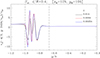 |
Fig. A.3. Distributions of the x speed at t = 340b/vAe along the y cut through the left tube center for a number of grid spacings as labeled. All computations pertain to the Sx motion for a fixed combination of physical parameters, [ρi/ρe = 5, ℓ/ℛ = 0.4, d/ℛ = 2.5, kb = π/30]. The computational domain size is fixed at [xM = 12b, yM = 10b]. Only the lower half (y ≤ 0) is shown for any y profile, the other half being symmetric about y = 0. The vertical dash-dotted lines delineate the borders of the nonuniform layer. |
where 𝒜(y) is some slow-varying envelope. Letting ωAi = kvAi be the internal Alfvén frequency, some instantaneous phase variation, ϕac(t) = (ωAe − ωAi)t, is therefore accumulated over the continuum, leading to Nhc = ⌊ϕac(t)/π⌋ half-cycles, with ⌊ ⋅ ⌋ being the floor function (see Shi et al. 2024, for similar applications). Consequently, one expects Nhc or Nhc + 1 extrema, where the uncertainty derives from the phase φ0 in Eq. (A.1). Plugging in the numbers yields a ϕac/π of 6.27, and therefore six or seven extrema are expected. This expectation is faithfully reproduced in Fig. A.3. The same can actually be said for all instants when the internal field behaves like a quasi-mode. Moving on to the portions outside the nonuniform layer, the only difference that one can barely tell for different Δ appears in the external flow fields immediately adjacent to the layer. On the other hand, no difference can be discerned in the internal motions.
Figure A.4 examines the grid spacing effect from the energetics perspective, differentiating Δ with different colors. Equations (12) to (15) are employed to evaluate all energetics-related quantities, and we take the area, Q, therein to be a box, [ − (d/2 + 1.2b),(d/2 + 1.2b)] × [ − 1.2b, 1.2b]. Figure A.4a performs a gross energy balance analysis over Q by presenting the temporal profiles of the time-derivative of the instantaneous total energy (dEtot/dt, solid curves) and those of the instantaneous energy flux into Q (−F, asterisks). The asterisks of different colors cannot be told apart, the reason being that all computations yield an identical set of dependents at the boundaries of Q. A difference nonetheless shows up among the solid curves, despite dEtot/dt being supposed to balance F (see Eq. 12). As was intuitively expected, gross energy conservation is maintained for a longer duration when a finer grid is employed, with a difference of ∼30% between dEtot/dt and −F staring to appear at t ∼ 90b/vAe (∼270b/vAe) when Δ = 0.01b (0.0025b). It should be noted that the examined Q is the union of three mutually exclusive portions; namely, the tube interiors (to be denoted as “int”), nonuniform layers (“layer”), and exterior (“ext”). Figure A.4b then displays, against time, the energies in these individual portions. By far the most significant effect that the grid spacing has on the energetics is that the energy in the nonuniform layer is increasingly underestimated when Δ increases. However, there exists only a weak difference among the Eext curves because only the flows in the immediate neighborhood of either tube are somehow impacted by the choices of Δ. Furthermore, the internal energies (Eint) consistently remain the same when Δ is varied, reinforcing the notion that Δ has no influence on the internal flow field.
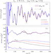 |
Fig. A.4. Temporal profiles of some energetics-related quantities for several grid spacings, as differentiated by different colors. Energetics are consistently examined for a box, [ − (d/2 + 1.2b),(d/2 + 1.2b)] × [ − 1.2b, 1.2b], in which the three mutually exclusive constituents are the tube interiors, nonuniform layers, and exterior. Shown in (a) are the time derivative of the total perturbation energy in the box (dEtot/dt, the solid curves), together with the instantaneous energy flux into this box (−F, asterisks). Further plotted in (b) are the instantaneous total energy in the interiors (Eint), nonuniform layers (Elayer), and the exterior (Eext). All computations pertain to the Sx pattern for a fixed combination of physical parameters [ρi/ρe = 5, ℓ/ℛ = 0.4, d/ℛ = 2.5, kb = π/30]. The computational domain size is fixed at [xM = 12b, yM = 10b]. |
All Tables
All Figures
|
Fig. 1. Schematics showing both the two-elliptic-tube configuration and lower-order kink motions therein. Illustrated in (b) are two identical tubes that have elliptic cross sections and that are separated in the x direction. The y − z plane is identified as the tube plane, the meaning of which is clearer in the curved representation in panel a. This study examines only two tube orientations (panels c and d), with the one labeled “x-major” (“x-minor”) corresponding to the situation where the major (minor) axis of either tube is aligned with the x axis. The tube centers are placed symmetrically with respect to the y axis. Only axial fundamentals are considered, making it possible to examine the three-dimensional (3D) wave fields with a 2D approach. Lower-order kink motions are classified according to their internal flow fields in the apex plane (panels c or d); hence, such symbols as Sx and Ay (see the text for more details). |
| In the text | |
|
Fig. 2. Kink motions in isolated tubes with circular cross sections for a fixed pair of density contrast and dimensionless axial wave numbers, [ρi/ρe = 3, kb = π/30]. A specific dimensionless layer width, |
| In the text | |
|
Fig. 3. Kink motions with (a) Sx and (b) Ax patterns in a two-circular-tube configuration. Plotted are the time sequences of the x speed sampled at the left tube center (vx(−d/2, 0; t), the solid curves) together with the best-fit damping envelopes (dashed). The time-dependent computations pertain to a fixed combination, [ρi/ρe = 5, ℓ/ℛ = 0.4, d/ℛ = 2.5, kb = π/30], with ℓ and ℛ being the nonuniform layer width and mean tube radius implemented by Ruderman & Roberts (2002), respectively. A fitting procedure with an exponentially damped cosine was performed over the duration exactly encompassing the extrema indicated by the red asterisks, even though the best-fit envelopes are plotted for the entire time interval. Kink motions are excited with the perturbation described by Eq. (20) with appropriate signs. |
| In the text | |
|
Fig. 4. Comparison of (a) the oscillation frequencies, Ω, and (b) the damping rates, γ, of ideal quasi-modes deduced from time-dependent computations (the open circles) with those expected with the T-matrix formalism (solid lines). We depict the results for the Sx and Ax patterns with different colors. The T-matrix curves are taken from Fig. 4 of Soler & Luna (2015, SL15). Shown here is how Ω and γ/Ω depend on ℓ/ℛ, while the rest of the parameters are fixed at [ρi/ρe = 5, d/ℛ = 2.5, kb = π/30]. The [ℓ/ℛ, d/ℛ] notations follow from SL15 for ease of comparison. |
| In the text | |
|
Fig. 5. Kink motions with (a) Sx and (b) Ax patterns in a two-elliptic-tube configuration with an x-major orientation. Plotted are the time sequences of the x speed sampled at the left tube center (vx(−d/2, 0; t), the solid curves) for a number of ratios of the semi-major to semi-minor axis (a/b) distinguished with different colors. A fitting procedure was performed for each sequence, over the duration encompassing the six extrema, starting with the one denoted by an asterisk. The best-fit damping envelope is plotted for the entire sequence, but only for a/b = 2.5 to avoid overcrowding the plots. The computations pertain to a fixed combination, |
| In the text | |
|
Fig. 6. Representative snapshots of the velocity field (the blue arrows) and energy density distribution (ϵ, filled contours) for (a) the Sx motion and (b) the Ax one in a two-elliptic-tube configuration with the x-major orientation. The inset in each panel emphasizes the distribution of ϵ in a representative nonuniform layer, whose boundaries are shown by the solid red curves. The white contour indicates where the Alfvén frequency, ωA = kvA, equals the quasi-mode frequency deduced with the fitting procedure. Both computations pertain to a fixed combination, |
| In the text | |
|
Fig. 7. Distributions of the x speed along the y cut through the left tube center at a number of instants as labeled. Panels a and b correspond to the Sx and Ax motions, respectively. The vertical dotted lines represent the borders of the nonuniform layer. Only the lower half (y < 0) of a y profile is displayed, the other half being symmetric with respect to y = 0. All computations were conducted for the x-major orientation with a fixed combination of physical parameters |
| In the text | |
|
Fig. 8. Dependencies of (a) the quasi-mode periods (P) and (b) damping-time-to-period ratios (τ/P) on the ratio of the semi-major to semi-minor axis (a/b) for kink motions in a two-elliptic-tube configuration with the x-major orientation. The Sx and Ax patterns are distinguished by the line styles. A number of dimensionless tube separations (d/b) are examined, as is differentiated by the different colors, with d/b constrained to avoid tube overlapping. All results pertain to a fixed combination of physical parameters, |
| In the text | |
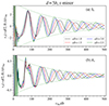 |
Fig. 9. Similar to Fig. 5 but for the x-minor orientation. |
| In the text | |
|
Fig. 10. Similar to Fig. 6 but for the x-minor orientation. The associated animation is available online. |
| In the text | |
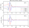 |
Fig. 11. Similar to Fig. 7 but for the x-minor orientation. |
| In the text | |
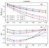 |
Fig. 12. Similar to Fig. 8 but for the x-minor orientation. |
| In the text | |
|
Fig. A.1. Temporal profiles of the x speed sampled at the left tube center (vx(−d/2, 0; t), the solid curves) for a number of domain sizes as labeled. Overplotted by the dashed curves are the best-fit damping envelopes. All computations pertain to the Sx motion for a fixed combination of physical parameters, [ρi/ρe = 5, ℓ/ℛ = 0.4, d/ℛ = 2.5, kb = π/30]. The grid spacing is fixed at Δ = 0.01b. |
| In the text | |
|
Fig. A.2. Temporal profiles of the x speed sampled at the left tube center for a number of grid spacings as labeled. All computations pertain to the Sx motion for a fixed combination of physical parameters, [ρi/ρe = 5, ℓ/ℛ = 0.4, d/ℛ = 2.5, kb = π/30]. The computational domain size is fixed at [xM = 12b, yM = 10b]. |
| In the text | |
|
Fig. A.3. Distributions of the x speed at t = 340b/vAe along the y cut through the left tube center for a number of grid spacings as labeled. All computations pertain to the Sx motion for a fixed combination of physical parameters, [ρi/ρe = 5, ℓ/ℛ = 0.4, d/ℛ = 2.5, kb = π/30]. The computational domain size is fixed at [xM = 12b, yM = 10b]. Only the lower half (y ≤ 0) is shown for any y profile, the other half being symmetric about y = 0. The vertical dash-dotted lines delineate the borders of the nonuniform layer. |
| In the text | |
|
Fig. A.4. Temporal profiles of some energetics-related quantities for several grid spacings, as differentiated by different colors. Energetics are consistently examined for a box, [ − (d/2 + 1.2b),(d/2 + 1.2b)] × [ − 1.2b, 1.2b], in which the three mutually exclusive constituents are the tube interiors, nonuniform layers, and exterior. Shown in (a) are the time derivative of the total perturbation energy in the box (dEtot/dt, the solid curves), together with the instantaneous energy flux into this box (−F, asterisks). Further plotted in (b) are the instantaneous total energy in the interiors (Eint), nonuniform layers (Elayer), and the exterior (Eext). All computations pertain to the Sx pattern for a fixed combination of physical parameters [ρi/ρe = 5, ℓ/ℛ = 0.4, d/ℛ = 2.5, kb = π/30]. The computational domain size is fixed at [xM = 12b, yM = 10b]. |
| In the text | |
Current usage metrics show cumulative count of Article Views (full-text article views including HTML views, PDF and ePub downloads, according to the available data) and Abstracts Views on Vision4Press platform.
Data correspond to usage on the plateform after 2015. The current usage metrics is available 48-96 hours after online publication and is updated daily on week days.
Initial download of the metrics may take a while.