| Issue |
A&A
Volume 684, April 2024
|
|
|---|---|---|
| Article Number | A154 | |
| Number of page(s) | 5 | |
| Section | The Sun and the Heliosphere | |
| DOI | https://doi.org/10.1051/0004-6361/202347786 | |
| Published online | 17 April 2024 | |
Horizontally polarized kink oscillations supported by solar coronal loops in an asymmetric environment⋆
1
Shandong Key Laboratory of Optical Astronomy and Solar-Terrestrial Environment, School of Space Science and Physics, Institute of Space Sciences, Shandong University, Weihai, Shandong 264209, PR China
e-mail: This email address is being protected from spambots. You need JavaScript enabled to view it.
2
Institute of Frontier and Interdisciplinary Science, Shandong University, Qingdao, Shandong 266237, PR China
Received:
23
August
2023
Accepted:
15
February
2024
Abstract
Context. Kink oscillations are ubiquitously observed in solar coronal loops, and understanding them is crucial in the contexts of coronal seismology and atmospheric heating.
Aims. We studied kink modes supported by a straight coronal loop embedded in an asymmetric environment using 3D magnetohydrodynamic simulations.
Methods. We implemented the asymmetric effect by setting different exterior densities below and above the loop interior and initiated the simulation using a kink-like velocity perturbation perpendicular to the loop plane, mimicking the frequently measured horizontally polarized kink modes.
Results. We find that the external velocity fields show fan-blade structures propagating in the azimuthal direction as a result of the successive excitation of higher azimuthal Fourier modes. Resonant absorption and phase-mixing can still occur despite an asymmetric environment, leading to the development of small-scale structures at loop boundaries. These small-scale structures nonetheless develop asymmetrically at the upper and lower boundaries due to the different gradients of the Alfvén speed.
Conclusions. These findings enrich our understanding of kink modes in coronal loops embedded within an asymmetric environment, providing insights that will be helpful for future high-resolution observations.
Key words: Sun: corona / Sun: oscillations
Movie associated to Fig. 3 is available at https://www.aanda.org
© The Authors 2024
 Open Access article, published by EDP Sciences, under the terms of the Creative Commons Attribution License (https://creativecommons.org/licenses/by/4.0), which permits unrestricted use, distribution, and reproduction in any medium, provided the original work is properly cited.
This article is published in open access under the Subscribe to Open model. This email address is being protected from spambots. You need JavaScript enabled to view it. to support open access publication.
1. Introduction
Magnetohydrodynamic (MHD) waves abound in the solar atmosphere (see reviews by, e.g., Li et al. 2020; Van Doorsselaere et al. 2020; Banerjee et al. 2021; Nakariakov et al. 2021; Wang et al. 2021). In particular, kink waves supported by the structured corona have attracted considerable attention since their first imaging detection (Aschwanden et al. 1999; Nakariakov et al. 1999). Further observations show that kink oscillations in coronal loops may be decaying (e.g., Zimovets & Nakariakov 2015; Goddard et al. 2016) or decayless (Tian et al. 2012; Wang et al. 2012; Nisticò et al. 2013; Anfinogentov et al. 2015). Ubiquitous propagating kink modes were also detected in the outer corona (Tomczyk et al. 2007; Van Doorsselaere et al. 2008). Studies of kink modes are often in the context of either coronal heating or coronal magnetic field diagnosis (e.g., Nakariakov & Ofman 2001; Yang et al. 2020). The two contexts are not mutually exclusive. As an example, Goddard & Nisticò (2020) connected the evolution of kink waves with the thermal evolution of their host loops.
A thorough understanding of kink modes is crucial for their related applications. In classical theories in which a straight coronal loop and a piecewise constant loop interior and loop exterior are assumed, kink modes are a collective eigenmode with azimuthal wavenumber q = 1 (e.g., Edwin & Roberts 1983). When a continuous transition layer connects the loop interior and exterior, kink modes are subject to resonant absorption (Goossens et al. 2011). During this process, the coordinated wave energy is transferred to localized Alfvénic motions, which subsequently phase-mix to generate small-scale structures. Along this line of thinking, a variety of modeling works have been performed to explore either the properties of kink modes or their heating effects (e.g., Antolin et al. 2015; Magyar & Van Doorsselaere 2016; Karampelas et al. 2017; Guo et al. 2019, 2020; Shi et al. 2021a,b; De Moortel & Howson 2022).
In reality, however, the environment of coronal loops is unlikely to be uniform, as is the case with the much-studied horizontally polarized kink modes (Wang et al. 2008). The upper and lower ambient coronae of the loop apex may be asymmetric due to density stratification. While the properties of MHD waves in an asymmetric slab configuration have been examined (e.g., Allcock & Erdélyi 2017; Zsámberger et al. 2018; Chen et al. 2022), there has been no study dedicated to collective waves supported by an asymmetric tube. This work examines the property of kink modes supported by a straight coronal loop in an asymmetric environment using 3D MHD simulations. We see new features in comparison with the case in which a symmetric ambient corona is implemented. Section 2 provides the numerical setup and is followed by the simulation results in Sect. 3. Section 4 provides a summary of this work.
2. Numerical setup
Our equilibrium configuration, illustrated in Fig. 1b, is a straightened version of a curved tube anchored in the photosphere (Fig. 1a). We see coronal loops as field-aligned magnetic tubes. The equilibrium magnetic field is z-directed, and all equilibrium quantities are z-independent. The equilibrium density is prescribed by
![Mathematical equation: $$ \begin{aligned} \rho (x,y) = \rho _{\rm e}(\theta )+\left[\rho _{\rm i} - \rho _{\rm e}(\theta )\right]f(r), \end{aligned} $$](/articles/aa/full_html/2024/04/aa47786-23/aa47786-23-eq1.gif) (1)
(1)
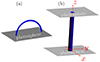 |
Fig. 1. Illustrations of a curved tube anchored in the photosphere (a) and its straightened version (b), which is used in our configuration. |
where (r, θ) denotes a standard polar coordinate system in the x − y plane, and the azimuthal coordinate, θ, is measured counterclockwise from the positive direction of the x-axis. A continuous profile, f(r) = exp[−(r/R)α], is used to connect the internal density, ρi = 5 × 10⁸ mp cm−3 (mp is the proton mass), to some external density, ρe(θ), with α = 6 and the nominal loop radius R = 1 Mm. This setup normalizes the length of the transition layer, l, to the loop radius as l/R ≈ 0.6, which is within the range of some seismological estimations based on resonant absorption (e.g., Arregui et al. 2007). We constructed an asymmetric background (hereafter the asymmetric case) by setting
 (2)
(2)
where [ρe1,ρe2] = [1,3.5] × 108 mp cm−3. Here ρe1 represents the density at (x, y) = (0, +∞) and ρe2 at (x, y) = (0, −∞). Figures 2a2 and b2 show the equilibrium density profiles along the x-axis (i.e., y = 0) and y-axis (i.e., x = 0) for this case. One sees that the loop environment is asymmetric in the y direction but symmetric in the x direction. The x (y) direction is shown as horizontal (vertical), in accordance with the convention in naming the polarization properties of kink motions (see Fig. 1a). The magnetic field was set to be uniform (15 G). The interior temperature at (x, y) = (0, 0) is Ti = 1 MK. A uniform thermal pressure was implemented to enforce transverse force balance, and the resulting plasma β is 0.0155. The pertinent Alfvén speeds are [vAi, vAe1, vAe2]=[1463, 3272, 1749] km s−1. The loop length is L = 50 Mm. A further simulation with the symmetric background (ρe1 = ρe2 = 1 × 10⁸ mp cm−3, hereafter the symmetric case) was conducted for comparison (Figs. 2a1 and b1).
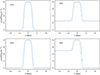 |
Fig. 2. Equilibrium density profiles along the x-axis (y = 0) and y-axis (x = 0) for the symmetric (left) and asymmetric case (right). |
For both cases, the equilibrium is perturbed by a horizontal kick,
 (3)
(3)
where v0 = 10 km s−1 is the amplitude, and σ = R characterizes the spatial extent. The z dependence in Eq. (3) dictates that only axial fundamentals are of interest here.
The set of ideal MHD equations was evolved using the PLUTO code (Mignone et al. 2007). We used the piecewise parabolic method for spatial reconstruction, and the second-order Runge–Kutta method for time-stepping. The Harten-Lax-van Leer discontinuities approximate Riemann solver (Miyoshi & Kusano 2005) was used to compute inter-cell fluxes, and a hyperbolic divergence cleaning method was used to keep the magnetic field divergence-free. We simulated only half of the loop, taking advantage of the symmetry with respect to the apex plane (z = L/2). The simulation domain is [ − 20, 20] Mm × [ − 20, 20] Mm × [0, 25] Mm in x, y, and z. In the x and y directions, we used 600 uniform grids for [ − 4, 4] Mm and 200 stretched grids for the other domains. A uniform grid with 50 cells was adopted in the z direction. We used the outflow boundary condition for all primitive variables at the lateral boundaries (x and y). The symmetric boundary condition was applied at the top boundary (z = L/2). For the bottom boundary (z = 0), the transverse velocities (vx and vy) were fixed at zero. The density, pressure, and Bz were fixed at their initial values. The other variables were set as outflows.
3. Simulation results
Figure 3 shows the density distributions together with the velocity fields in the apex plane at t = 130 s for the symmetric (top panels) and asymmetric (bottom) cases. The left column displays these quantities for a large domain, while the right column zooms in on the inner portion. From Fig. 3 and the associated animation, one sees that the velocity field for the symmetric case is typical of azimuthally standing kink motions. The development of vortical motions, a result of resonant absorption and phase-mixing, is clear at the loop boundary. For the asymmetric case, one sees the development of fan-blade-like motions propagating azimuthally. Furthermore, the velocity fields at the upper and lower loop boundaries are quite different, with small-scale structures much easier to identify at the upper boundary.
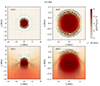 |
Fig. 3. Density distributions and velocity fields at the loop apex for the symmetric (top) and asymmetric (bottom) cases at t = 130 s. The dashed green lines mark a circle of radius r = 2 Mm. The right panels show zoomed-in views of the left ones. An animated version of this figure is available online; it has the same layout and runs from 0 to 400 s. |
We can further see the difference between the velocity fields of the two cases by examining their radial velocities, vr. Figure 4 shows the temporal evolution of vr along a circle of radius r = 2 Mm in the apex plane (the dashed lines in Fig. 3). For the symmetric case (a), azimuthally standing motions are clearly shown. For the asymmetric case (b), however, vr is seen to propagate in the azimuthal direction as the velocity stripes become increasingly inclined with time. Put another way, Fourier modes with increasingly high azimuthal wave numbers appear as time proceeds.
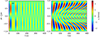 |
Fig. 4. Temporal evolution of the radial velocity, vr, along the circle delineated in Fig. 3 for the symmetric (a) and asymmetric (b) cases. |
We then decomposed the radial velocity, vr, shown in Fig. 4 into different Fourier modes. Following Terradas et al. (2018), this decomposition was performed using the discrete Fourier transform,
 (4)
(4)
where Gvr(q) represents the coefficient of Fourier mode q, N is the length of the discrete vr sequence, and vr(n) is the nth element. The real (imaginary) part of Gvr nearly vanishes for even (odd) q values given that vr is almost symmetric about the y-axis. The Fourier coefficients are displayed in Fig. 5 as functions of q and time. For the symmetric case, only a single Fourier mode of q = 1 is recognizable, with Gvr(q = 1) being almost purely real (Fig. 5a). For the asymmetric case, however, Fourier modes with higher q values are excited. Figure 5b displays the real or imaginary parts of Gvr(q) for four selected Fourier modes. One finds that the Fourier coefficients of higher q modes reach their maximum at later stages, indicating a coupling among different Fourier modes. The modulus |Gvr(q)| as a function of q and time is displayed in the bottom panels for the symmetric (c) and asymmetric (d) cases. Similarly, one sees a single Fourier mode of q = 1 in the symmetric case. For the asymmetric case, multiple Fourier modes coexist and higher q modes are successively excited as time proceeds. These results demonstrate that the fan-blade-like velocity fields propagating in the azimuthal direction are attributable to the continuous excitation of higher Fourier modes and the coupling among these modes.
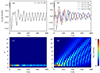 |
Fig. 5. Fourier coefficients, Gvr, for the symmetric (left) and asymmetric (right) cases. Top panels show the real or imaginary part of Gvr for some selected q as a function of time. Bottom panels show the modulus |Gvr| as a function of time and q. |
We verified that wave energy is well contained in the system after a brief transient phase. The kink mode is then subject to damping due to resonant absorption and the subsequent phase-mixing (Goossens et al. 2011). This process manifests itself as the vortical motions and the development of small-scale structures at loop boundaries. The top panels of Fig. 6 show the temporal evolution of vx along the y-axis in the apex plane (z = L/2). For the symmetric case (a1), small-scale spikes are symmetrically developing at both sides of the loop boundary. For the asymmetric case, however, spikes develop more rapidly at the upper boundary than at the lower one. This difference is further demonstrated in the bottom panels of Fig. 6, where two snapshots of vx (t = 200 s and 400 s) are displayed. We compared our results with the theoretical prediction given by Mann et al. (1995), and our phase-mixing length, Lph, is estimated as
 (5)
(5)
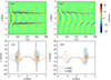 |
Fig. 6. Temporal evolution of vx(x = 0, y, z = L/2) for the symmetric (a1) and asymmetric (b1) cases. The profiles of vx(x = 0, y, z = L/2) at two different times are displayed for the symmetric (a2) and asymmetric (b2) cases. |
where ωA = (π/L)vA(x, y) is the local Alfvén frequency. That small-scale structures develop more rapidly at the upper boundary is therefore due to the stronger gradient in the Alfvén frequency therein. We proceeded more quantitatively by evaluating the Alfvén frequencies [ωAi, ωAe1, ωAe2]≈[0.09, 0.21, 0.11] rad s−1 with the corresponding densities. We first examined the Alfvén continuum pertinent to the upper loop boundary. Equation (20) from Mann et al. (1995) indicates that the instantaneous phase variation across the continuum is Δφ1 = (ωAe1 − ωAi)t, meaning that the number of spikes is approximately Nspikes, 1 ≈ Δφ1/π. Our setup then yields that ∼7.6 spikes are accumulated every 200 s, which is in line with Fig. 6b2. Likewise, one expects that ∼1.3 extrema will be accumulated every 200 s close to the lower loop boundary, which is also quantitatively reproduced.
The development of small-scale structures is accompanied by the damping of coordinated kink motions. The damping envelope of kink modes has been extensively examined given their seismological potential (e.g., Ruderman & Roberts 2002; Pascoe et al. 2012; Hood et al. 2013). Here we only focused on the difference in terms of the period and damping times between asymmetric and symmetric cases. Figure 7 presents the temporal evolution of vx averaged over the region of ρ > 0.9ρi for the symmetric (a) and asymmetric cases (b; labeled “sym” and “asym”). We fit the profiles using an exponentially damped sinusoid, printing the best-fit periods (P) and damping times (τ). One sees that Pasym > Psym, which is unsurprising given the overall heavier ambient corona and hence a larger inertia experienced by the kink motions in the asymmetric case. The fact that τasym > τsym can be understood by drawing an analogy with the damping of kink motions in an axisymmetric setup, for which the ideal quasi-mode (QM) theory predicts that τ/P in the thin-boundary-thin-tube limit decreases with the ratio of the internal density, ρi, to the ambient value, ρamb (e.g., Goossens et al. 1992; Ruderman & Roberts 2002). While it is not straightforward to quantify, ρamb in the asymmetric case is expected to exceed ρe1, which can be unambiguously identified as ρamb in the symmetric case. That said, an exponential damping envelope does not apply to the symmetric case at late times (Fig. 7a), reinforcing the notion that ideal QMs offer only a partial picture of the time-dependent coordinated motions (see Soler & Terradas 2015, for details).
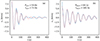 |
Fig. 7. Temporal profiles of vx (averaged over the loop center with ρ > 0.9ρi) for the symmetric (a) and asymmetric (b) cases. The dashed red lines are the best-fit exponential damped sinusoids, with the fitted period, P, and damping time, τ, displayed in each panel. |
The profile of vx in the symmetric case (Fig. 7a) shows a beat at t ≈ 160 s. One possible cause of this beat is the interplay between kink motions and Alfvénic motions (e.g., Fig. 9 of Soler & Terradas 2015). It is known that the presence of similar beats can lead to an underestimation of the actual damping time (Nisticò et al. 2013). We therefore also computed the period (PQM) and damping time (τQM) expected for kink QMs resonantly absorbed in the Alfvén continuum (see the review by Goossens et al. 2011 for conceptual clarifications). We specifically adapted our previous resistive eigenmode code (Chen et al. 2021) to address the present equilibrium configuration, finding PQM ≈ 51.6 s and τQM ≈ 67.1 s. These QM values are rather close to the best-fit values in Fig. 7a (Psym and τsym), suggesting that the presence of a beat-like behavior may not significantly affect our fitting approach for evaluating the kink periods and damping times.
In this work we paid attention to the effect of an asymmetric loop environment on kink oscillations, and thus neglected both gravity and the gravitationally stratified atmosphere to avoid further complexity. The density profile we adopted (Eq. (2)) may not exactly represent a realistic stratified density profile. In terms of modeling, however, our model is different from most previous simulations, in which a uniform background was assumed. The results shown here are relevant for further exploring more realistic models.
It is necessary to mention that for the asymmetric case, the density variation in the environment (ρe2/ρe1 = 3.5) across the loop width is more significant than the density variations over a scale height (Λ ≈ 50 Mm) of a 1 MK corona. While we did not attempt to model a stratified density profile, we nonetheless performed an additional simulation with ρe2 = 1.2 × 10⁸ mp cm−3. This density ratio of ρe2/ρe1 = 1.2 is in line with some loops observed by the Transition Region and Coronal Explorer (TRACE) or Solar and Heliospheric Observatory (SOHO), whose width, w, can be as large as 8 Mm (i.e., exp(w/Λ)≈1.21; e.g., Schrijver 2007). We performed similar analyses, and their results are shown in Figs. 8 and 9. We find that the key features we previously obtained, the azimuthally propagating velocity field and the excitation of higher azimuthal Fourier modes, still exist, though not as strong as in the case with ρe2/ρe1 = 3.5. Our model thus provides a proof-of-concept test of the effect of an asymmetric environment on kink oscillations. More realistic models that take both the stratified atmosphere and the gravity effect into account are called for.
4. Summary
We studied kink modes supported by a straight coronal loop in an asymmetric environment using 3D MHD simulations. The new features compared with the case of symmetric ambients are summarized as follows:
-
(1)
The velocity fields in the exterior show the development of fan-blade features that propagate azimuthally. This is attributed to the successive excitation of higher azimuthal Fourier modes.
-
(2)
Resonant absorption and phase-mixing can still occur in the asymmetric case. Velocity spikes are generated non-symmetrically, with small-scale structures developing more rapidly at the upper boundary than at the lower.
This work provides a simplified model that studies horizontally polarized kink modes supported by coronal loops in an asymmetric ambient corona. These findings enrich our understanding of kink modes in more realistic configurations and are helpful for future high-resolution observations.
Movie
Movie 1 associated with Fig. 3 (fig3anim) Access Supplementary Material
Note that a nominal loop radius, R = 1 Mm, serves essentially as a normalizing constant in our gravity-free modeling. The key dynamics here result primarily from the deviation of the dimensionless ρe2/ρe1 from unity. As such, the ensuing results are equally applicable upon proper scaling (see Sect. 4.1.2 of Goedbloed et al. 2019, for more on this aspect).
Acknowledgments
This work is supported by the National Natural Science Foundation of China (12273019, 41974200, 42230203, 12373055, 41904150). We gratefully acknowledge ISSI-BJ for supporting the international team “Magnetohydrodynamic wavetrains as a tool for probing the solar corona”.
References
- Allcock, M., & Erdélyi, R. 2017, Sol. Phys., 292, 35 [NASA ADS] [CrossRef] [Google Scholar]
- Anfinogentov, S. A., Nakariakov, V. M., & Nisticò, G. 2015, A&A, 583, A136 [NASA ADS] [CrossRef] [EDP Sciences] [Google Scholar]
- Antolin, P., Okamoto, T. J., De Pontieu, B., et al. 2015, ApJ, 809, 72 [Google Scholar]
- Arregui, I., Andries, J., Van Doorsselaere, T., Goossens, M., & Poedts, S. 2007, A&A, 463, 333 [NASA ADS] [CrossRef] [EDP Sciences] [Google Scholar]
- Aschwanden, M. J., Fletcher, L., Schrijver, C. J., & Alexander, D. 1999, ApJ, 520, 880 [Google Scholar]
- Banerjee, D., Krishna Prasad, S., Pant, V., et al. 2021, Space Sci. Rev., 217, 76 [NASA ADS] [CrossRef] [Google Scholar]
- Chen, S.-X., Li, B., Van Doorsselaere, T., et al. 2021, ApJ, 908, 230 [NASA ADS] [CrossRef] [Google Scholar]
- Chen, S.-X., Li, B., Guo, M., Shi, M., & Yu, H. 2022, ApJ, 940, 157 [NASA ADS] [CrossRef] [Google Scholar]
- De Moortel, I., & Howson, T. A. 2022, ApJ, 941, 85 [NASA ADS] [CrossRef] [Google Scholar]
- Edwin, P. M., & Roberts, B. 1983, Sol. Phys., 88, 179 [Google Scholar]
- Goddard, C. R., & Nisticò, G. 2020, A&A, 638, A89 [NASA ADS] [CrossRef] [EDP Sciences] [Google Scholar]
- Goddard, C. R., Nisticò, G., Nakariakov, V. M., & Zimovets, I. V. 2016, A&A, 585, A137 [NASA ADS] [CrossRef] [EDP Sciences] [Google Scholar]
- Goedbloed, H., Keppens, R., & Poedts, S. 2019, Magnetohydrodynamics of Laboratory and Astrophysical Plasmas (Cambridge: Cambridge University Press) [Google Scholar]
- Goossens, M., Hollweg, J. V., & Sakurai, T. 1992, Sol. Phys., 138, 233 [Google Scholar]
- Goossens, M., Erdélyi, R., & Ruderman, M. S. 2011, Space Sci. Rev., 158, 289 [Google Scholar]
- Guo, M., Van Doorsselaere, T., Karampelas, K., et al. 2019, ApJ, 870, 55 [Google Scholar]
- Guo, M., Li, B., & Van Doorsselaere, T. 2020, ApJ, 904, 116 [Google Scholar]
- Hood, A. W., Ruderman, M., Pascoe, D. J., et al. 2013, A&A, 551, A39 [NASA ADS] [CrossRef] [EDP Sciences] [Google Scholar]
- Karampelas, K., Van Doorsselaere, T., & Antolin, P. 2017, A&A, 604, A130 [NASA ADS] [CrossRef] [EDP Sciences] [Google Scholar]
- Li, B., Antolin, P., Guo, M. Z., et al. 2020, Space Sci. Rev., 216, 136 [NASA ADS] [CrossRef] [Google Scholar]
- Magyar, N., & Van Doorsselaere, T. 2016, A&A, 595, A81 [NASA ADS] [CrossRef] [EDP Sciences] [Google Scholar]
- Mann, I. R., Wright, A. N., & Cally, P. S. 1995, J. Geophys. Res., 100, 19441 [Google Scholar]
- Mignone, A., Bodo, G., Massaglia, S., et al. 2007, ApJS, 170, 228 [Google Scholar]
- Miyoshi, T., & Kusano, K. 2005, J. Comput. Phys., 208, 315 [NASA ADS] [CrossRef] [Google Scholar]
- Nakariakov, V. M., & Ofman, L. 2001, A&A, 372, L53 [NASA ADS] [CrossRef] [EDP Sciences] [Google Scholar]
- Nakariakov, V. M., Ofman, L., Deluca, E. E., Roberts, B., & Davila, J. M. 1999, Science, 285, 862 [Google Scholar]
- Nakariakov, V. M., Anfinogentov, S. A., Antolin, P., et al. 2021, Space Sci. Rev., 217, 73 [NASA ADS] [CrossRef] [Google Scholar]
- Nisticò, G., Nakariakov, V. M., & Verwichte, E. 2013, A&A, 552, A57 [NASA ADS] [CrossRef] [EDP Sciences] [Google Scholar]
- Pascoe, D. J., Hood, A. W., de Moortel, I., & Wright, A. N. 2012, A&A, 539, A37 [NASA ADS] [CrossRef] [EDP Sciences] [Google Scholar]
- Ruderman, M. S., & Roberts, B. 2002, ApJ, 577, 475 [Google Scholar]
- Schrijver, C. J. 2007, ApJ, 662, L119 [NASA ADS] [CrossRef] [Google Scholar]
- Shi, M., Van Doorsselaere, T., Guo, M., et al. 2021a, ApJ, 908, 233 [Google Scholar]
- Shi, M., Van Doorsselaere, T., Antolin, P., & Li, B. 2021b, ApJ, 922, 60 [NASA ADS] [CrossRef] [Google Scholar]
- Soler, R., & Terradas, J. 2015, ApJ, 803, 43 [Google Scholar]
- Terradas, J., Magyar, N., & Van Doorsselaere, T. 2018, ApJ, 853, 35 [Google Scholar]
- Tian, H., McIntosh, S. W., Wang, T., et al. 2012, ApJ, 759, 144 [Google Scholar]
- Tomczyk, S., McIntosh, S. W., Keil, S. L., et al. 2007, Science, 317, 1192 [Google Scholar]
- Van Doorsselaere, T., Nakariakov, V. M., & Verwichte, E. 2008, ApJ, 676, L73 [Google Scholar]
- Van Doorsselaere, T., Srivastava, A. K., Antolin, P., et al. 2020, Space Sci. Rev., 216, 140 [Google Scholar]
- Wang, T. J., Solanki, S. K., & Selwa, M. 2008, A&A, 489, 1307 [NASA ADS] [CrossRef] [EDP Sciences] [Google Scholar]
- Wang, T., Ofman, L., Davila, J. M., & Su, Y. 2012, ApJ, 751, L27 [Google Scholar]
- Wang, T., Ofman, L., Yuan, D., et al. 2021, Space Sci. Rev., 217, 34 [CrossRef] [Google Scholar]
- Yang, Z., Bethge, C., Tian, H., et al. 2020, Science, 369, 694 [Google Scholar]
- Zimovets, I. V., & Nakariakov, V. M. 2015, A&A, 577, A4 [NASA ADS] [CrossRef] [EDP Sciences] [Google Scholar]
- Zsámberger, N. K., Allcock, M., & Erdélyi, R. 2018, ApJ, 853, 136 [Google Scholar]
All Figures
|
Fig. 1. Illustrations of a curved tube anchored in the photosphere (a) and its straightened version (b), which is used in our configuration. |
| In the text | |
|
Fig. 2. Equilibrium density profiles along the x-axis (y = 0) and y-axis (x = 0) for the symmetric (left) and asymmetric case (right). |
| In the text | |
|
Fig. 3. Density distributions and velocity fields at the loop apex for the symmetric (top) and asymmetric (bottom) cases at t = 130 s. The dashed green lines mark a circle of radius r = 2 Mm. The right panels show zoomed-in views of the left ones. An animated version of this figure is available online; it has the same layout and runs from 0 to 400 s. |
| In the text | |
|
Fig. 4. Temporal evolution of the radial velocity, vr, along the circle delineated in Fig. 3 for the symmetric (a) and asymmetric (b) cases. |
| In the text | |
|
Fig. 5. Fourier coefficients, Gvr, for the symmetric (left) and asymmetric (right) cases. Top panels show the real or imaginary part of Gvr for some selected q as a function of time. Bottom panels show the modulus |Gvr| as a function of time and q. |
| In the text | |
|
Fig. 6. Temporal evolution of vx(x = 0, y, z = L/2) for the symmetric (a1) and asymmetric (b1) cases. The profiles of vx(x = 0, y, z = L/2) at two different times are displayed for the symmetric (a2) and asymmetric (b2) cases. |
| In the text | |
|
Fig. 7. Temporal profiles of vx (averaged over the loop center with ρ > 0.9ρi) for the symmetric (a) and asymmetric (b) cases. The dashed red lines are the best-fit exponential damped sinusoids, with the fitted period, P, and damping time, τ, displayed in each panel. |
| In the text | |
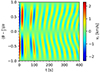 |
Fig. 8. Same as Fig. 4b, but for the case of ρe2 = 1.2 × 10⁸ mp cm−3. |
| In the text | |
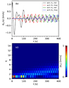 |
Fig. 9. Same as the right column of Fig. 5, but for the case of ρe2 = 1.2 × 10⁸ mp cm−3. |
| In the text | |
Current usage metrics show cumulative count of Article Views (full-text article views including HTML views, PDF and ePub downloads, according to the available data) and Abstracts Views on Vision4Press platform.
Data correspond to usage on the plateform after 2015. The current usage metrics is available 48-96 hours after online publication and is updated daily on week days.
Initial download of the metrics may take a while.