| Issue |
A&A
Volume 686, June 2024
|
|
|---|---|---|
| Article Number | A96 | |
| Number of page(s) | 8 | |
| Section | Extragalactic astronomy | |
| DOI | https://doi.org/10.1051/0004-6361/202349064 | |
| Published online | 03 June 2024 | |
Revisiting the abundance pattern and charge-exchange emission in the centre of M 82
Department of Physics, Tokyo University of Science, 1-3 Kagurazaka, Shinjuku-ku, Tokyo 162-8601, Japan
e-mail: This email address is being protected from spambots. You need JavaScript enabled to view it.
Received:
22
December
2023
Accepted:
18
March
2024
Abstract
Context. The interstellar medium (ISM) in starburst galaxies contains many chemical elements that are synthesised by core-collapse supernova explosions. By measuring the abundances of these metals, we can study the chemical enrichment within the galaxies and the transportation of metals into the circumgalactic environment through powerful outflows.
Aims. We performed a spectral analysis of the X-ray emissions from the core of M 82 using the Reflection Grating Spectrometer (RGS) on board XMM-Newton to accurately estimate the metal abundances in the ISM.
Methods. We analysed over 300 ks of RGS data observed with 14 position angles, covering a cross-dispersion width of 80 arcsec. We employed multi-temperature thermal plasma components in collisional ionisation equilibrium (CIE) to reproduce the observed spectra, each of which exhibited a different spatial broadening.
Results. The O VII band CCD image shows a broader distribution that those for the O VIII and Fe-L bands. The O VIII line profiles have a prominent double-peaked structure that corresponds to the north- and southward outflows. The O VII triplet feature exhibits marginal peaks. A single CIE component that is convolved with the O VII band image approximately reproduces the spectral shape. A CIE model combined with a charge-exchange emission model also successfully reproduces the O VII line profiles. However, the ratio of these two components varies significantly with the observed position angles, which is physically implausible. Spectral fitting of the broadband spectra suggests a multi-temperature phase in the ISM that is approximated by three components at 0.1, 0.4, and 0.7 keV. Notably, the 0.1 keV component exhibits a broader distribution than the 0.4 and 0.7 keV plasmas. The derived abundance pattern shows super-solar N/O, solar Ne/O and Mg/O, and half-solar Fe/O ratios. These results indicate the chemical enrichment by core-collapse supernovae in starburst galaxies.
Key words: astrochemistry / ISM: abundances / galaxies: ISM / galaxies: clusters: individual: M 82 / galaxies: starburst / X-rays: ISM
© The Authors 2024
 Open Access article, published by EDP Sciences, under the terms of the Creative Commons Attribution License (https://creativecommons.org/licenses/by/4.0), which permits unrestricted use, distribution, and reproduction in any medium, provided the original work is properly cited.
This article is published in open access under the Subscribe to Open model. This email address is being protected from spambots. You need JavaScript enabled to view it. to support open access publication.
1. Introduction
Core-collapse supernovae (CCSNe) from massive star progenitors play a crucial role in the evolution of galaxies. They are primary sources of light α-elements such as O, Ne, and Mg (e.g., Nomoto et al. 2013). Additionally, they heat the interstellar medium (ISM) to X-ray-emitting temperatures. In starburst galaxies, in particular, in regions of active star formation, CCSNe can induce powerful winds from the galactic disc. These winds, also known as outflows, are essential in the enrichment of the circumgalactic medium that connects the ISM to the local Universe (Orlitova 2020, for a comprehensive review). Consequently, X-ray observations of starburst galaxies offer valuable insights into the processes supplying energy and metals into both the ISM and circumgalactic space.
In recent years, numerous X-ray observations have focused on the extended X-ray-emitting ISM in starburst galaxies (e.g., Strickland et al. 2004; Yamasaki et al. 2009; Konami et al. 2012; Mitsuishi et al. 2013; Yang et al. 2020). The M 82 galaxy, a well-established starburst system located at a distance of 3.53 Mpc from our Solar System (1′∼1 kpc; Karachentsev et al. 2004), has been a key object in these studies. The nearly edge-on appearance makes this galaxy an ideal laboratory for studying biconical outflows that erupt from the central region of the galaxy (e.g., Strickland & Heckman 2009; Zhang 2018). These outflows exhibit a multi-phase structure that is observed in the infrared, Hα, and X-ray windows (Strickland et al. 1997; Lehnert et al. 1999; Read & Stevens 2002; Engelbracht et al. 2006; Zhang et al. 2014; Lopez et al. 2020). Strickland & Heckman (2007) found diffuse Fe Heα emission in the central regions, suggesting the presence of gas at temperatures of several kiloelectronvolts. Additionally, strong emission lines of elements such as O, Mg, Si, S, and Fe have been detected from the core to the wind regions of the galaxy (e.g., Tsuru et al. 1997, 2007; Ranalli et al. 2008; Konami et al. 2011). In the central regions, these elements show an unusual abundance pattern: super-solar ratios of Ne/O and Mg/O (> 1.5 solar) with super-solar O/Fe ratios have been reported (e.g., Tsuru et al. 1997; Ranalli et al. 2008; Konami et al. 2011; Zhang et al. 2014). This contradicts the pre-existing nucleosynthesis models of CCSN (e.g., Nomoto et al. 2013). In contrast, the outflowing gas outside the disc shows an abundance pattern consistent with CCSN predictions (Tsuru et al. 2007; Konami et al. 2011).
An additional exciting feature in M 82 is the charge exchange (CX) X-ray emission. In this process, one or more electrons are transferred from a cold neutral atom to a hot ion. Subsequently, the cascade relaxation of this captured electron from a highly excited energy state to the ground state of the ion results in the X-ray line emission (e.g., Cravens 2002; Sibeck et al. 2018; Gu & Shah 2023). A notable feature of the CX process is present in the O VII triplet structure: the forbidden line at 0.56 keV is enhanced compared to the resonance line at 0.57 keV. In starburst galaxies, CX emission at the fronts of hot gas flows that collide with cold matter is expected to be observed. Liu et al. (2012) analysed the data from the Reflection Grating Spectrometer (RGS) on board XMM-Newton and reported this enhancement in the O VII triplet in several starburst galaxies, suggesting a significant CX contribution in addition to plasma in a collisional ionisation equilibrium (CIE) state. Konami et al. (2011) and Lopez et al. (2020) included the CX component in their analysis of the CCD spectra from M 82, although their spectral resolution was too limited to sufficiently resolve the O VII triplet. Zhang et al. (2014) used the RGS data from an XMM-Newton observation of M 82 and estimated that the interaction area between the neutral and ionised matter is significantly larger than the geometric surface area of the galaxy.
The RGS on board XMM-Newton is effective for our study. It offers a good spatial and spectral resolution within the ∼0.5−2 keV band. This makes it particularly useful for measuring α-element abundances and estimating the CX contribution. However, any line structures in the dispersed spectra are practically broadened when the source extends ≳0.8 arcmin, leading to decreased resolving power for extended objects such as galaxies (Mao et al. 2023, for a recent review). Therefore, careful treatment is required in an analysis of the RGS spectra of galaxies, especially for the broadening effect on each emission line (e.g., Chen et al. 2018; Yang et al. 2020; Fukushima et al. 2023). In this study, we used deep 300 ks RGS data obtained with different position angles to model the spectra of the central region of M 82 to determine its temperature structure, the CX contribution, and the abundance pattern. The paper is structured as follows. Section 2 summarises the XMM-Newton observations and data reduction. In Sect. 3, we outline the line-broadening effect intrinsic to the RGS analysis. Section 4 presents the general prescription for our fitting and the results. We discuss and interpret our findings in Sect. 5. We assumed the cosmological parameters to be H0 = 70 km s−1 Mpc−1, Ωm = 0.3, and ΩΛ = 0.7. The proto-solar abundance of Lodders et al. (2009) was adopted to estimate the element abundances.
2. Observations and data reduction
We analysed the archival observation data of the M 82 centre with RGS, which is installed on XMM-Newton. Table 1 summarises the observations used in this work. The M 82 nucleus (Lester et al. 1990) is located near the centre of the MOS detector for these observations. The RGS data were processed using the task rgsproc that is wrapped in the XMM-Newton Science Analysis System (SAS) version 18.0.0. We obtained light curves from the CCD9 on the RGS focal plane (den Herder et al. 2001). Next, the mean count rate μ and standard deviation σ were derived by fitting these curves with a Gaussian. In order to discard soft-proton background flares, a count-rate threshold of μ ± 2σ was applied to uncleaned events. Following the SAS team, other standard screening criteria were employed. The cleaned exposure times of each observation are listed in Table 1.
RGS observations.
3. Imaging analysis
In Figs. 1a–c, we show X-ray images of the centre of M 82 for the O VII (Fig. 1a, 0.55−0.60 keV), O VIII Lyα (Fig. 1b, 0.64−0.67 keV), and Fe-L (Fig. 1c, 0.70−1.20 keV) bands. Avoiding the relatively high noise in the O VII band image, we subtracted the continuum counts from the raw events. Point-like sources were not discarded. In these images, the outflows extending from the disc towards the south-east and north-west are visible, especially in Figs. 1a and b. The dispersion directions for the three representative position angles are overlaid. The cross-dispersion width of 80 arcsec covers a significant part of the two outflow regions. Incorporating data from different position angles helps to resolve the degeneracy between the energy and spatial position along the dispersion angle, allowing for a more detailed analysis of the outflow structure.
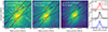 |
Fig. 1. X-ray images of M 82 and line profiles in the three energy bands. (a) Mosaiced X-ray count image of the centre of M 82 in the O VII (0.55−0.60 keV) band by CCDs. The three representative RGS position angles are overlaid on the 80 arcsec cross-dispersion widths. The arrows indicate the dispersion direction in which the photons are scattered into the higher-energy side. The star and the solid line passing through it indicate the centre and disc of M 82 (Lester et al. 1990; Mayya et al. 2005). The continuum flux estimated using the 0.45−0.55 keV band is subtracted from the raw count image. (b), (c) Same as panel a, but in the O VIII Lyα (0.64−0.67 keV) and Fe-L (0.70−1.20 keV) bands. (d) Normalised count profiles projected onto the 138° dispersion axis in the 0.55−0.60 keV (O VII), 0.64−0.67 keV (O VIII), and 0.70−1.20 keV (dominated by Fe-L lines) bands. The angular offset is measured in reference to the star in panel a, where the positive side of the offset axis is the higher-energy part in diffracted spectra. (e), (f) Same as panel d, but along the dispersion axes of 296° and 319°, respectively. |
The X-ray count profiles within a cross-dispersion width of 80 arcsec along each dispersion axes are given in Figs. 1d–f. These profiles show significant differences in the three bandpasses. In particular, the Fe-L line band is characterised by a centrally peaked and narrow distribution on a spatial scale of 1−2 arcmin. In contrast, the O VII band exhibits the most strongly broadened profiles. In both the O VII and O VIII profiles, a dip is observed at ∼1 arcmin offset northward from the galaxy centre. The two peaks next to the dip correspond to the outflows towards the southeast and northeast. This bimodal line profile in the O band along the centrally peaked distribution in the Fe-L line band was reported by Zhang et al. (2014). The appearances of this double-peak structure, especially in the O VIII band profile, depend on the dispersion direction (Figs. 1d and f).
4. Spectral analysis
4.1. General prescription
The RGS spectra along the dispersion direction can be used within a cross-dispersion width of 5 arcmin centred on the MOS detector (e.g., Zhang et al. 2019; Narita et al. 2023). After filtering the cleaned event files with XDSP_CORR columns using evselect, we extracted first-order RGS spectra from the cross-dispersion width of 80 arcsec centred on the nucleus of M 82 with the task rgsspectrum. This method takes advantage of the accurately determined rectangular cross-dispersion limits1 compared to the standard RGS analysis with xpsf- options of rgsproc, for instance (e.g., Fukushima et al. 2022, 2023). The cross-dispersion widths and dispersion directions for three representative position angles are plotted in Figs. 1a–c. The RGS1 and RGS2 spectra and response matrices were co-added through the rgscombine script.
The RGS instrument is primarily designed for observing point-like sources; therefore, the response matrices generated by the standard SAS method are not suitable for analysing diffuse emissions from various extended sources, such as SN remnants, galaxies, and clusters (e.g., Chen et al. 2018; Tateishi et al. 2021; Fukushima et al. 2023). Line broadening in a first-order RGS spectrum is observed as ΔE = 0.138Δθ, where ΔE and Δθ represent the line broadening and the spatial extent in the wavelength (Å) and dispersion (arcmin) axes, respectively. To fit the RGS spectra of these extended sources, it is necessary to convolve the response matrix with the projected surface-brightness profile along the dispersion direction (e.g., Tamura & Ohta 2004; Mao et al. 2023). Moreover, variations in spatial broadening across different energy bands necessitate applying different convolution scales for distinct spectral components. The differences in the spatial distribution of the O VII, O VIII, and Fe-L band images (Sect. 3) imply the presence of multiple thermal CIE components with different spatial scales. Zhang et al. (2014) analysed the RGS spectra of M 82 by adopting two spectral broadenings: bimodal soft emission, and centrally peaked hard emission. We further test different spatial broadenings below for the spectral components emitting the O VII and O VIII lines.
We used the XSPEC package version 12.10.1f (Arnaud 1996), but with the revised ATOMDB version 3.0.9 (Smith et al. 2001; Foster et al. 2012) that provides information on the line and continuum emission at 201 temperatures from 8.6 × 10⁻⁴ to 86 keV. This updated ATOMDB is standard in XSPEC version 12.11.0k or later2. The C-statistic method (Cash 1979) was adopted in our spectral fitting to estimate the spectral parameters and their error ranges without bias (Kaastra 2017). Each spectrum was re-binned to have a minimum of 1 count per spectral bin.
4.2. Spectral models
In our RGS spectral analysis, we reproduced the diffuse ISM emission (denoted by ISMM 82). Two individual absorptions modify the ISMM 82 component. We assumed 6.7 × 1020 cm−2 for the Galactic extinction (Willingale et al. 2013). The intrinsic absorption of M 82 for diffuse emissions typically is (1 − 3)×1021 cm−2 (e.g., Konami et al. 2011; Zhang et al. 2014); thus, we used the fixed value 2 × 1021 cm−2. The photoelectric absorption cross-sections were retrieved from Verner et al. (1996). Letting these absorption parameters free to vary does not significantly change the results we demonstrate below. We did not include diffuse astrophysical background emission such as the cosmic X-ray background or Milky Way halo component in our spectral fitting since they only contribute to the observed RGS spectra as flat components. A power-law component was introduced to account for increasing flux at energies below 0.5 keV. We used another power-law component with a 1.6 photon index (Ranalli et al. 2008) subjected to 2 × 1022 cm−2 extinction to take the point-source emission into account.
The complete model applied to the observed spectra is represented as phabsGal × (phabsM 82 × ISMM 82 + phabsPS × powerlawPS)+powerlawBKG. To account for the line-broadening effect on ISMM 82 described in Sects. 1 and 3, we used the XSPEC model rgsxsrc with mosaiced CCD (MOS+pn) images in specific bands. We first performed spectral fits in two local bands: the O VIII band (0.60−0.77 keV, Sect. 4.3), and the O VII band (0.45−0.62 keV, Sect. 4.4), each convolved with the respective images. Then, we fit the broadband spectra covering the full RGS energy range of 0.45−1.75 keV (hereafter broadband; Sect. 4.5), using the image of this band, which closely resembles the Fe-L band image. The spatial distribution of each emission line may not precisely match the image of its corresponding energy band because these bands also include continuum emission. The image convolution approach in this study is an approximation, as was also applied in similar works, and the resulting systematic uncertainties are discussed below.
4.3. Results for the O VIII Lyα line
First, we tested the thermal plasma component in collisional ionisation equilibrium (CIE) convolved with the O VIII band image: ISMM 82 = vapec (the CIE modelling). We ignored the point-source contribution because the absorption for the point sources at the centre of M 82 is quite strong (≳1 × 1022 cm−2; e.g. Brightman et al. 2016). Despite focusing on local line structures, in the spectral fittings, we used a wider energy range of 0.60−0.77 keV, including the Fe XVII line around 0.73 keV. This approach enabled a more robust measurement of global parameters such as kT; a restriction to local fits led to poorly constrained values (e.g., Lakhchaura et al. 2019). The combined spectrum of each observation was fitted with free parameters of kT, the emission measure (EM), and the O and Fe abundances.
The CIE modelling approximately reproduces the observed spectra (Fig. 2a), achieving good C-statistics/d.o.f. values ≲1.2 (the x-axes of Fig. 3a). However, a spectral sub-peak corresponding to the northward wind region at ∼0.65 keV and ∼0.66 keV for the position angles of 138° and 319°, respectively, appears narrower than the spectral model convolved with the O VIII band image. The derived kTCIE values are plotted against the RGS position angle in Fig. 3b, yielding a uniform kTCIE with a median of 0.49 keV and a 16–84th percentile range of 0.47−0.53 keV.
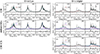 |
Fig. 2. RGS spectra of the centre of M 82 in the O VIII (a), (b) and O VII (c)–(e) bands for the three representative position angles. The best-fitting models and the data-to-model ratios for the three methods are plotted: the CIE modelling convolved with local band images (the first row), the shifted-CIEs modelling convolved by the broadband image (the second row), and the CIE+CX modelling convolved with the O VII band image (the third row, only for the O VII lines). The positions of the O VII forbidden and resonance lines are labelled in the 319° panel of c. |
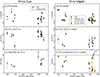 |
Fig. 3. Some parameters of the O VIII and O VII bands plotted against the RGS position angle. (a) C-stat./d.o.f. values from the CIE and shifted-CIEs modellings on the 0.60−0.77 keV band (O VIII and Fe XVII). (b) Temperatures derived from the two modellings. (c) EMS/EMN profile obtained from the shifted-CIEs method. (d) Same as (a), but on the 0.45−0.62 keV band fitting (N VII and O VII). The results are from the CIE, shifted-CIEs (0.14 keV), and CIE+CX modellings. (e) Temperatures derived from the CIE modelling. (f) Flux contribution of the CX components to the O VII line. |
Figure 3 shows that the O VIII Lyα consists of a main peak and a sub-peak ∼5 eV away from it, whose intensities depend on the RGS dispersion direction. The 5 eV separation between the two peaks at ∼0.66 keV corresponds to an angular diameter of 1 arcmin along the dispersion direction (Fig. 1b). To reproduce this double-peak structure, we then tried two spatially distinct components with varying redshift parameters to represent different spatial positions: ISMM 82 = vapecN + vapecS (the shifted-CIEs modelling). The subscripts N and S represent the northeast and southwest emission peaks, respectively. The temperature and metal abundances of the two components were assumed to have the same values. Each CIE component was convolved with the broadband image (0.45−1.75 keV) as the extent of each peak is similar to that of the Fe-L band (Figs. 1d–f). While our subscript nomenclature is not an a priori assumption, it describes the observed spectral features, including the sub-peak structure for the northward wind (Fig. 2b). Good C-stat./d.o.f. values are derived on the O VIII line (Fig. 3a). This model yields similar temperatures as the CIE modelling (Fig. 3b). The EMS/EMN ratios are greater than unity for all position angles (Fig. 3c): The brighter vapecS is shifted to the harder side and softer side when the dispersion angle is inverted (Fig. 2b). This variation naturally arises due to minor differences among RGS slices. Thus, our shifted-CIEs method successfully and reasonably approximates the spatial variation and broadening of the O VIII Lyα line; that is, the double CIE modelling with the broadband image can be a substitute for an actual emission plasma broadened as the O VIII band image.
4.4. Results for the O VII triplet lines
For the O VII triplet feature, we also started with the CIE modelling with the O VII band image: ISMM 82 = vapec. We also ignored the point-source contribution due to the same reason described in Sect. 4.3. Following the same assumptions as for the analysis of the O VIII Lyα band, we used the 0.45−0.62 keV band, including the N VII line at 0.5 keV. The spectra were fitted with free parameters of kT, the EM, and the N and O abundances. As shown in Fig. 2c, the best-fit CIE models convolved with the O VII band image closely resemble the observed line profile of O VII. We obtained good C-stat./d.o.f. for all dispersions (the x-axes of Fig. 3d). A hint of residuals is seen at the forbidden line energy of 0.56 keV, although their significance is relatively tiny. For example, in the 319° angle, which exhibits the highest residual, it remains at ∼3σ. The CIE modelling for O VII provides a uniform kTCIE across the position angles, as does the O VIII band modelling (Fig. 3e). The median value and 16–84th percentile range for kTCIE are 0.14 keV and 0.11−0.18 keV, respectively.
Next, we applied the shifted-CIEs modelling for O VII and took its marginal bimodality into account: ISMM 82 = vapecN + vapecS. Each CIE component was convolved with the broad RGS bandpass (0.45−1.75 keV). Considering the relatively widespread O VII profile (Figs. 1d–f), we adopted the additional broadening option of the APEC model. We set the temperature of the two CIE components to kT = 0.14 keV based on the results of the CIE modelling. This model effectively fits the broadened O VII lines (Fig. 2d), yielding C-stat./d.o.f. values similar to those from the CIE modellings (Fig. 3d). The significance of the residuals at 0.56 keV decreased to 2σ at most. For certain datasets, including that for the position angle of 296°, a single CIE component is sufficient to represent the spectra, where the dominant component likely corresponds to the bright southwest outflow.
The hint of residuals at 0.56 keV might be attributable to the CX emission. To constrain the contribution of the CX component, we employed the second version of the AtomDB CX Model ACX (Smith et al. 2014), together with a CIE plasma: ISMM 82 = vapec + vacx (the CIE+CX modelling). Both components were convolved in this model with the O VII band image. The collision velocity between ions and atoms was set to moderate values 200 km s−1 (e.g., Cumbee et al. 2016; Zhang 2018). We assumed that the CIE and CX components shared the same temperature (and abundance), and we tested two temperature assumptions of kT = 0.1 and 0.2 keV. The CIE+CX model also gives fine-fits for all spectra under both temperature assumptions (Figs. 2e and 3d). However, this CIE+CX modelling still resulted in similar residuals around the forbidden line at a level of ∼2σ at most. Additionally, Fig. 3f shows that at certain position angles, the CX emission significantly exceeds the CIE contribution, and vice versa. It reaches up to 96% at 319°. There is no clear correlation between the CX fraction and position angle; for example, similar angles yield significantly different CX fractions. The lack of a consistent pattern leads to the conclusion that the CIE+CX models may not be physically plausible.
The minor residuals observed at 0.56 keV correspond to the energy of the forbidden line of O VII for the bright southward wind component. We attempted to introduce a spatially narrower CX component to fill the residuals. We modified the CIE+CX model by replacing the broader CX component with a more localised and less broadened one. This modified model did not change our results and did not improve the spectral fits, which makes it challenging to assert reliably that the CX emission is based on the current RGS data. Okon et al. (2024) recently discussed a possible localised CX emission. However, they introduced a different model in which the low-energy side of the observed spectrum was attributed predominantly to the CX emission.
4.5. Results for the broadband spectra
Finally, we fit the broadband RGS spectra (0.45−1.75 keV) without the CX model. Our adopted model was ISMM 82 = vapechot + vapecwarmN + vapecwarmS + vapeccoolN + vapeccoolS. All of the CIE components were convolved with the broadband image. As described in Sects. 4.3 and 4.4, two CIEs for the cool and warm plasma, when convolved with the broadband image, effectively reproduce the local band spectra. These gas components mainly contribute to the O VII and O VIII lines, with the new hot component mainly accounting for the Fe-L and Mg lines. In this model, kThot, kTwarm, and EMs of each component varied freely under the assumption that kTwarmN = kTwarmS. We fixed kTcool to 0.14 keV. The N, O, Ne, Mg, Fe, and Ni abundances were free parameters with shared values in all spectral components, and other metals were set to 1 solar. Unfortunately, firm constraints on the Ni abundance are not very promising since clear Ni line structures are rarely detected by RGS, even in highly metal-rich systems (e.g. the Centaurus cluster; Sanders et al. 2008; Fukushima et al. 2022). The intrinsic absorption for the hot plasma in M 82, which is more substantial than for the warm and cool gases (see Sect. 4.1), is difficult to constrain. Hence, we adopted 8 × 1021 cm−2 for the hot-component extinction, consistent with the intrinsic absorption estimated for the hot gases in the CCD study (kT ≳ 0.7 keV, Lopez et al. 2020). The other prescriptions for the warm and cool components followed those with each shifted-CIEs modelling (Sects. 4.3 and 4.4). Despite this slightly simplistic modelling, the mean values of the cool+warm and hot-gas absorptions are close to fixed values when they were allowed to vary.
The best-fitting models for the representative broad-band spectra of M 82 are shown in Fig. 4. As we designed, each CIE component contributes to observed emission lines. This model yields good fits with excellent C-stat./d.o.f. values up to 1.1 for all observations (Fig. 5a). In Fig. 5b, we plot the derived kThot and kTwarm against the position angles. We obtain the medians and 16–84th percentile ranges as kThot = 0.70 (0.68−0.74) keV and kTwarm = 0.41 (0.40−0.43) keV. The inclusion of the hot gas in the Fe-L lines results in a slight decrease in the kTwarm value compared to the results from the shifted-CIEs method for the local O VIII band. Figure 5c reveals uniform values for the relative EMs of each temperature plasma. Here, the hot component dominates more strongly than the other two, with the warm and cool gases at similar intensities. The abundance ratios N/O, Ne/O, Mg/O, and Fe/O are also uniform in the dataset: super-solar N/O, solar ratios of Ne/O and Mg/O, and sub-solar Fe/O (Fig. 5d). The Ni values are not plotted due to large errors and scattering, as we described above. In particular, the solar abundance ratios of light α-elements near the disc are reported for the first time. They are discussed in more detail in Sect. 5.3.
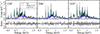 |
Fig. 4. Best-fitting models for the broadband RGS spectra of the centre of M 82 for the three position angles. The thin dotted and solid lines represent the background and point-source components, respectively (see Sect. 4.1). |
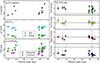 |
Fig. 5. Some parameters of the broad-band fitting plotted against the RGS position angle. (a) C-stat./d.o.f. values from the 0.45−1.75 keV band fitting. (b) Temperatures of the warm and hot components. (c) Relative EM/EMhot ratios for the cool and warm plasmas. (d) Abundance ratios of N/O (vertical ties), Ne/O (ninja-stars), Mg/O (pentagons), and Fe/O (horizontal ties). |
5. Discussion
5.1. Multi-temperature phase in the centre of M 82
In our analysis of the RGS spectra from multiple position angles, we determined that the hot (0.7 keV), warm (0.4 keV), and cool (0.1−0.2 keV) components effectively represent the temperature structure of the ISM in M 82. The 0.6−0.7 keV component, which causes the Mg (and possibly Si) emission lines, was also reported in studies using RGS and CCD data (Read & Stevens 2002; Origlia et al. 2004; Konami et al. 2011; Zhang et al. 2014; Lopez et al. 2020). A warm plasma component with kT ∼ 0.5 keV was also identified by Ranalli et al. (2008). The presence of another cool gas contribution was predicted through line diagnostics of the O VII triplet, suggesting kT ∼ 0.1 − 0.3 keV, (Ranalli et al. 2008). Such a cool component at the core of M 82 was not reported (e.g., Zhang et al. 2014; Lopez et al. 2020), only an indication of the 0.2 keV component (Konami et al. 2011, CCD study). The O VII emission has often been interpreted to be a result of the CX processes (e.g., Zhang et al. 2014). However, in our spectral model, which accounts for different spatial broadenings for O VII and O VIII, the CIE components are the primary contributors to these line emissions.
Observational and simulation studies generally predict that the core regions of starburst galaxies undergo a multi-temperature phase of gas, ranging from cold dust to hot outflows (e.g., Leroy et al. 2015). Interestingly, a multi-phase state like this is also applicable to X-ray-emitting gas itself (e.g., Melioli et al. 2013; Schneider et al. 2018). This theoretical prediction agrees well with the plasma content that we revealed for M 82, as well as with other starburst galaxies (e.g. NGC 3079, Konami et al. 2012; Arp 299, Mao et al. 2021). Furthermore, even in the Milky Way, certain regions with a high concentration of massive stars, such as superbubbles, possess intermixed X-ray plasma with different temperatures (e.g. Kim et al. 2017 for simulations; Fuller et al. 2023 for observations). The multi-phase ISM would be ubiquitous in star-forming regions, regardless of their scale. While the origin of the different spatial variations of the cool and warm components eludes our present study, we expect it to be examined more robustly through high-resolution observation of M 82.
5.2. Note for the CX emission
Previous reports of the CX emission from M 82 focused on the limited position angle (mainly the 319° observation; Liu et al. 2011; Zhang et al. 2014). At this angle, the O VII profile expands toward the low-energy scale (Figs. 1d and f). This expansion was interpreted as high R- or G-ratio values3 in energy space. The enhancement in the soft part of the O VII triplet is likely due to the bright outflow towards the southeast, as discussed in Sect. 4.4. While our current results do not strongly favour CX emission, we considered its contribution in M 82 using the 319° result that is most significantly contaminated by the CX emission, if any. We assumed that the CX and CIE components share the same spatial distribution, although a more localised CX emission can be considered as well (Sect. 4.4). From this observation, we obtained an ACX normalisation of (3.3 ± 1.0)×10−4 cm−5. According to the study of M 51 by Yang et al. (2020), we can evaluate the spatial scale of the CX reaction from this ACX normalisation as
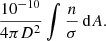 (1)
(1)
Here, D, n, and σ are the angular diameter distance to M 82, the density of receiver ions in the CX reaction and the CX cross sections, respectively. Assuming a spherical volume with a radius of 40 arcsec (∼0.67 kpc at M 82), we adopted n = 0.19 cm−3 from the CIE modelling in Sect. 4.4. The cross sections were set as σ = 5 × 10⁻¹⁵ cm2 (Gu & Shah 2023, and references therein). In consequence, we obtained the CX emitting area A = 14 ± 3 kpc2, which is an order of magnitude larger than the assumed surface area ∼1.5 kpc2. Similar illustrations were reported by Zhang et al. (2014) for the same centre of M 82 and by Yang et al. (2020) for M 51. This significant discrepancy makes us suspicious about the brightness of the CX emission if the broadened CX component is a dominant source of the O VII triplet lines. Okon et al. (2024) proposed that the CX component accounts for 40−60% of the O VII flux using a multi-temperature model, which is substantially lower than the previous estimate (∼90%, Zhang et al. 2014). The CX emission properties in M 82, such as the luminosity or the spatial extent, must be observed continuously to be challenged or validated more confidently with high-resolution and non-dispersive X-ray spectroscopic data from XRISM, which observes in orbit.
5.3. Metal abundance pattern
The metal abundance pattern is a key to studying the chemical enrichment process of observed gases. Figure 6 shows the median values and the 16–84th percentile ranges of N/O, Ne/O, Mg/O, and Fe/O at all position angles. For comparison, we also plot the Ni/O value, which might agree with Fe/O within a large error. We obtained solar-like ratios of the Ne/O and Mg/O that are lower than the results of two earlier RGS works (Ranalli et al. 2008; Zhang et al. 2014). Other studies with CCD reported super-solar patterns of light α-elements (e.g., Konami et al. 2011). The presence or absence of the CX contribution does not change the super-solar abundances in these studies. The primary origin of these gaps would be our modelling of the O VII and O VIII lines rather than the CX emission, which improves the estimation of a temperature structure in M 82. In particular, the inclusion of the cool-gas component would be essential progress in measuring the element abundances.
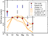 |
Fig. 6. Observed X/O abundance pattern from the broad-band spectral fits, where the medians and 16–84th percentile ranges for all dispersion angles are plotted. Two literature values from previous RGS works are given for comparison. The dashed line represents the solar composition. The solid thick and thin lines indicate the IMF-weighted yields predicted by Nomoto et al. (2013) and Sukhbold et al. (2016), respectively, assuming initially solar metallicity for the progenitors. The dashed lines are for each option of the mass-cutoff integration (< 25 M⊙). |
In Fig. 6, we compare the observed abundance pattern in the centre of M 82, a starburst system, with nucleosynthesis models of CCSNe. This comparison is crucial because most SNe in these systems are expected to originate from massive stars. We adopted two models: the classical standard yield by Nomoto et al. (2013), and the latest N20 calculations by Sukhbold et al. (2016). For both models, we assumed the initial mass function (IMF) by Salpeter (1955) with progenitor masses up to 40 M⊙. In addition, based on the discussion of the missing progenitor mass problem for CCSNe by Smartt (2015), we also employed another IMF-weighted integration with an upper mass limit of 25 M⊙.
For α-elements, the yields with Nomoto et al. (2013) most closely match the observed Ne/O and Mg/O ratios, but tend to underestimate those of Fe/O and Ni/O. For the case with an upper mass limit of 25 M⊙, the half-solar Fe/O and Ni/O values are explained well by both Nomoto et al. (2013) and Sukhbold et al. (2016). In the powerful starburst galaxy Arp 299, Mao et al. (2021) provided a similar picture by comparing the model yields to the N/O, Ne/O, Mg/O, S/O, and Ni/O pattern. However, the observed Fe/O and Ni/O ratios in M 82 might also be explained by including a minor contribution from Type Ia SNe (only 6% of the total SNe in the core of M 82). The hot ISM in M 82, as in other starburst galaxies, serves as a significant repository of CCSN products.
None of these CCSN models adequately reproduces the N/O ratio ∼2 solar in M 82. Similarly high N/O ratios have been reported in more ancient systems, such as early-type galaxies, including brightest cluster galaxies (e.g., Mao et al. 2019; Fukushima et al. 2023). These objects owe a dominant fraction of their N enrichment to mass-loss winds from massive and asymptotic giant branch stars. These mass-loss channels therefore likely contribute to the enrichment observed in the core of M 82, in addition to CCSNe. One caveat is that the N VII Lyα line is present at ∼0.5 keV and is likely to be affected by, for example, the estimate of the absorption for the cool+warm component and/or the contribution of the background emission (Sect. 4). When the gate valve is opened, the XRISM data will provide us a great opportunity to constrain the N abundance more robustly.
Alternatively, one can use the rgsregions task to do this if specifying a rectangle that is roughly symmetrical about the detector centre. Otherwise, users are strongly urged to check the generated RMFs and effective areas.
These ratios are given as f/i (R) and (i + f)/r (G), where r, f, and i are the flux of the resonance, forbidden, and intercombination lines, respectively.
Acknowledgments
The authors would like to thank Dr. D. Wang for taking the time to read our manuscript thoroughly as a reviewer and for providing helpful comments and suggestions. K.F. shall deem it an honour to be supported by the Japan Society for the Promotion of Science (JSPS) through Grants-in-Aid for Scientific Research (KAKENHI) grant Nos. 21J21541 and 22KJ2797 (Grant-in-Aid for JSPS Fellows). This work is based on observations obtained with XMM-Newton, an ESA science mission with instruments and contributions directly funded by ESA Member States and NASA of the USA. The XMM-Newton Science Archive (https://nxsa.esac.esa.int/nxsa-web/) stores and distributes the RGS data analysed in this paper. We get the second version of ACX from the ATOMDB website (http://www.atomdb.org/CX/) and run it on the PYXSPEC module implemented in the XSPEC package. The figures in this paper are generated using VEUSZ (https://veusz.github.io) and PYTHON (https://www.python.org).
References
- Arnaud, K. A. 1996, in Astronomical Data Analysis Software and Systems V, eds. G. H. Jacoby, & J. Barnes, ASP Conf. Ser., 101, 17 [NASA ADS] [Google Scholar]
- Brightman, M., Harrison, F. A., Barret, D., et al. 2016, ApJ, 829, 28 [CrossRef] [Google Scholar]
- Cash, W. 1979, ApJ, 228, 939 [Google Scholar]
- Chen, Y., Wang, Q. D., Zhang, G.-Y., Zhang, S., & Ji, L. 2018, ApJ, 861, 138 [NASA ADS] [CrossRef] [Google Scholar]
- Cravens, T. E. 2002, Science, 296, 1042 [CrossRef] [Google Scholar]
- Cumbee, R. S., Liu, L., Lyons, D., et al. 2016, MNRAS, 458, 3554 [NASA ADS] [CrossRef] [Google Scholar]
- den Herder, J. W., Brinkman, A. C., Kahn, S. M., et al. 2001, A&A, 365, L7 [NASA ADS] [CrossRef] [EDP Sciences] [Google Scholar]
- Engelbracht, C. W., Kundurthy, P., Gordon, K. D., et al. 2006, ApJ, 642, L127 [NASA ADS] [CrossRef] [Google Scholar]
- Foster, A. R., Ji, L., Smith, R. K., & Brickhouse, N. S. 2012, ApJ, 756, 128 [Google Scholar]
- Fukushima, K., Kobayashi, S. B., & Matsushita, K. 2022, MNRAS, 514, 4222 [NASA ADS] [CrossRef] [Google Scholar]
- Fukushima, K., Kobayashi, S. B., & Matsushita, K. 2023, ApJ, 953, 112 [NASA ADS] [CrossRef] [Google Scholar]
- Fuller, C. A., Kaaret, P., Bluem, J., et al. 2023, ApJ, 943, 61 [NASA ADS] [CrossRef] [Google Scholar]
- Gu, L., & Shah, C. 2023, in High-Resolution X-ray Spectroscopy: Instrumentation, Data Analysis, and Science, eds. C. Bambi, & J. Jiang (Singapore: Springer Nature), 255 [Google Scholar]
- Kaastra, J. S. 2017, A&A, 605, A51 [NASA ADS] [CrossRef] [EDP Sciences] [Google Scholar]
- Karachentsev, I. D., Karachentseva, V. E., Huchtmeier, W. K., & Makarov, D. I. 2004, AJ, 127, 2031 [Google Scholar]
- Kim, C.-G., Ostriker, E. C., & Raileanu, R. 2017, ApJ, 834, 25 [Google Scholar]
- Konami, S., Matsushita, K., Tsuru, T. G., Gandhi, P., & Tamagawa, T. 2011, PASJ, 63, S913 [CrossRef] [Google Scholar]
- Konami, S., Matsushita, K., Gandhi, P., & Tamagawa, T. 2012, PASJ, 64, 117 [CrossRef] [Google Scholar]
- Lakhchaura, K., Mernier, F., & Werner, N. 2019, A&A, 623, A17 [NASA ADS] [CrossRef] [EDP Sciences] [Google Scholar]
- Lehnert, M. D., Heckman, T. M., & Weaver, K. A. 1999, ApJ, 523, 575 [CrossRef] [Google Scholar]
- Leroy, A. K., Walter, F., Martini, P., et al. 2015, ApJ, 814, 83 [Google Scholar]
- Lester, D. F., Carr, J. S., Joy, M., & Gaffney, N. 1990, ApJ, 352, 544 [NASA ADS] [CrossRef] [Google Scholar]
- Liu, J., Mao, S., & Wang, Q. D. 2011, MNRAS, 415, L64 [NASA ADS] [CrossRef] [Google Scholar]
- Liu, J., Wang, Q. D., & Mao, S. 2012, MNRAS, 420, 3389 [NASA ADS] [CrossRef] [Google Scholar]
- Lodders, K., Palme, H., & Gail, H. P. 2009, in Astronomy, Astrophysics, and Cosmology, ed. J. Trümper (Berlin, Heidelberg: Springer), 560 [Google Scholar]
- Lopez, L. A., Mathur, S., Nguyen, D. D., Thompson, T. A., & Olivier, G. M. 2020, ApJ, 904, 152 [Google Scholar]
- Mao, J., de Plaa, J., Kaastra, J. S., et al. 2019, A&A, 621, A9 [NASA ADS] [CrossRef] [EDP Sciences] [Google Scholar]
- Mao, J., Zhou, P., Simionescu, A., et al. 2021, ApJ, 918, L17 [CrossRef] [Google Scholar]
- Mao, J., Paerels, F., Guainazzi, M., & Kaastra, J. S. 2023, in High-Resolution X-ray Spectroscopy: Instrumentation, Data Analysis, and Science, eds. C. Bambi, & J. Jiang (Singapore: Springer Nature), 9 [Google Scholar]
- Mayya, Y. D., Carrasco, L., & Luna, A. 2005, ApJ, 628, L33 [NASA ADS] [CrossRef] [Google Scholar]
- Melioli, C., de Gouveia Dal Pino, E. M., & Geraissate, F. G. 2013, MNRAS, 430, 3235 [NASA ADS] [CrossRef] [Google Scholar]
- Mitsuishi, I., Yamasaki, N. Y., & Takei, Y. 2013, PASJ, 65, 44 [CrossRef] [Google Scholar]
- Narita, T., Uchida, H., Yoshida, T., Tanaka, T., & Tsuru, T. G. 2023, ApJ, 950, 137 [CrossRef] [Google Scholar]
- Nomoto, K., Kobayashi, C., & Tominaga, N. 2013, ARA&A, 51, 457 [CrossRef] [Google Scholar]
- Okon, H., Smith, R. K., Picquenot, A., & Foster, A. R. 2024, ApJ, 963, 147 [NASA ADS] [CrossRef] [Google Scholar]
- Origlia, L., Ranalli, P., Comastri, A., & Maiolino, R. 2004, ApJ, 606, 862 [NASA ADS] [CrossRef] [Google Scholar]
- Orlitova, I. 2020, in Reviews in Frontiers of Modern Astrophysics, eds. P. Kabáth, D. Jones, & M. Skarka (Cham: Springer), 379 [CrossRef] [Google Scholar]
- Ranalli, P., Comastri, A., Origlia, L., & Maiolino, R. 2008, MNRAS, 386, 1464 [CrossRef] [Google Scholar]
- Read, A. M., & Stevens, I. R. 2002, MNRAS, 335, L36 [NASA ADS] [CrossRef] [Google Scholar]
- Salpeter, E. E. 1955, ApJ, 121, 161 [Google Scholar]
- Sanders, J. S., Fabian, A. C., Allen, S. W., et al. 2008, MNRAS, 385, 1186 [NASA ADS] [CrossRef] [Google Scholar]
- Schneider, E. E., Robertson, B. E., & Thompson, T. A. 2018, ApJ, 862, 56 [NASA ADS] [CrossRef] [Google Scholar]
- Sibeck, D. G., Allen, R., Aryan, H., et al. 2018, Space Sci. Rev., 214, 79 [NASA ADS] [CrossRef] [Google Scholar]
- Smartt, S. J. 2015, PASA, 32, e016 [NASA ADS] [CrossRef] [Google Scholar]
- Smith, R. K., Brickhouse, N. S., Liedahl, D. A., & Raymond, J. C. 2001, ApJ, 556, L91 [Google Scholar]
- Smith, R. K., Foster, A. R., Edgar, R. J., & Brickhouse, N. S. 2014, ApJ, 787, 77 [NASA ADS] [CrossRef] [Google Scholar]
- Strickland, D. K., & Heckman, T. M. 2007, ApJ, 658, 258 [NASA ADS] [CrossRef] [Google Scholar]
- Strickland, D. K., & Heckman, T. M. 2009, ApJ, 697, 2030 [Google Scholar]
- Strickland, D. K., Ponman, T. J., & Stevens, I. R. 1997, A&A, 320, 378 [NASA ADS] [Google Scholar]
- Strickland, D. K., Heckman, T. M., Colbert, E. J. M., Hoopes, C. G., & Weaver, K. A. 2004, ApJS, 151, 193 [Google Scholar]
- Sukhbold, T., Ertl, T., Woosley, S. E., Brown, J. M., & Janka, H. T. 2016, ApJ, 821, 38 [NASA ADS] [CrossRef] [Google Scholar]
- Tamura, N., & Ohta, K. 2004, MNRAS, 355, 617 [NASA ADS] [CrossRef] [Google Scholar]
- Tateishi, D., Katsuda, S., Terada, Y., et al. 2021, ApJ, 923, 187 [NASA ADS] [CrossRef] [Google Scholar]
- Tsuru, T. G., Awaki, H., Koyama, K., & Ptak, A. 1997, PASJ, 49, 619 [NASA ADS] [CrossRef] [Google Scholar]
- Tsuru, T. G., Ozawa, M., Hyodo, Y., et al. 2007, PASJ, 59, 269 [NASA ADS] [Google Scholar]
- Verner, D. A., Ferland, G. J., Korista, K. T., & Yakovlev, D. G. 1996, ApJ, 465, 487 [Google Scholar]
- Willingale, R., Starling, R. L. C., Beardmore, A. P., Tanvir, N. R., & O’Brien, P. T. 2013, MNRAS, 431, 394 [Google Scholar]
- Yamasaki, N. Y., Sato, K., Mitsuishi, I., & Ohashi, T. 2009, PASJ, 61, S291 [NASA ADS] [CrossRef] [Google Scholar]
- Yang, H., Zhang, S., & Ji, L. 2020, ApJ, 894, 22 [NASA ADS] [CrossRef] [Google Scholar]
- Zhang, D. 2018, Galaxies, 6, 114 [NASA ADS] [CrossRef] [Google Scholar]
- Zhang, S., Wang, Q. D., Ji, L., et al. 2014, ApJ, 794, 61 [NASA ADS] [CrossRef] [Google Scholar]
- Zhang, S., Wang, Q. D., Foster, A. R., et al. 2019, ApJ, 885, 157 [CrossRef] [Google Scholar]
All Tables
All Figures
|
Fig. 1. X-ray images of M 82 and line profiles in the three energy bands. (a) Mosaiced X-ray count image of the centre of M 82 in the O VII (0.55−0.60 keV) band by CCDs. The three representative RGS position angles are overlaid on the 80 arcsec cross-dispersion widths. The arrows indicate the dispersion direction in which the photons are scattered into the higher-energy side. The star and the solid line passing through it indicate the centre and disc of M 82 (Lester et al. 1990; Mayya et al. 2005). The continuum flux estimated using the 0.45−0.55 keV band is subtracted from the raw count image. (b), (c) Same as panel a, but in the O VIII Lyα (0.64−0.67 keV) and Fe-L (0.70−1.20 keV) bands. (d) Normalised count profiles projected onto the 138° dispersion axis in the 0.55−0.60 keV (O VII), 0.64−0.67 keV (O VIII), and 0.70−1.20 keV (dominated by Fe-L lines) bands. The angular offset is measured in reference to the star in panel a, where the positive side of the offset axis is the higher-energy part in diffracted spectra. (e), (f) Same as panel d, but along the dispersion axes of 296° and 319°, respectively. |
| In the text | |
|
Fig. 2. RGS spectra of the centre of M 82 in the O VIII (a), (b) and O VII (c)–(e) bands for the three representative position angles. The best-fitting models and the data-to-model ratios for the three methods are plotted: the CIE modelling convolved with local band images (the first row), the shifted-CIEs modelling convolved by the broadband image (the second row), and the CIE+CX modelling convolved with the O VII band image (the third row, only for the O VII lines). The positions of the O VII forbidden and resonance lines are labelled in the 319° panel of c. |
| In the text | |
|
Fig. 3. Some parameters of the O VIII and O VII bands plotted against the RGS position angle. (a) C-stat./d.o.f. values from the CIE and shifted-CIEs modellings on the 0.60−0.77 keV band (O VIII and Fe XVII). (b) Temperatures derived from the two modellings. (c) EMS/EMN profile obtained from the shifted-CIEs method. (d) Same as (a), but on the 0.45−0.62 keV band fitting (N VII and O VII). The results are from the CIE, shifted-CIEs (0.14 keV), and CIE+CX modellings. (e) Temperatures derived from the CIE modelling. (f) Flux contribution of the CX components to the O VII line. |
| In the text | |
|
Fig. 4. Best-fitting models for the broadband RGS spectra of the centre of M 82 for the three position angles. The thin dotted and solid lines represent the background and point-source components, respectively (see Sect. 4.1). |
| In the text | |
|
Fig. 5. Some parameters of the broad-band fitting plotted against the RGS position angle. (a) C-stat./d.o.f. values from the 0.45−1.75 keV band fitting. (b) Temperatures of the warm and hot components. (c) Relative EM/EMhot ratios for the cool and warm plasmas. (d) Abundance ratios of N/O (vertical ties), Ne/O (ninja-stars), Mg/O (pentagons), and Fe/O (horizontal ties). |
| In the text | |
|
Fig. 6. Observed X/O abundance pattern from the broad-band spectral fits, where the medians and 16–84th percentile ranges for all dispersion angles are plotted. Two literature values from previous RGS works are given for comparison. The dashed line represents the solar composition. The solid thick and thin lines indicate the IMF-weighted yields predicted by Nomoto et al. (2013) and Sukhbold et al. (2016), respectively, assuming initially solar metallicity for the progenitors. The dashed lines are for each option of the mass-cutoff integration (< 25 M⊙). |
| In the text | |
Current usage metrics show cumulative count of Article Views (full-text article views including HTML views, PDF and ePub downloads, according to the available data) and Abstracts Views on Vision4Press platform.
Data correspond to usage on the plateform after 2015. The current usage metrics is available 48-96 hours after online publication and is updated daily on week days.
Initial download of the metrics may take a while.