| Issue |
A&A
Volume 686, June 2024
|
|
|---|---|---|
| Article Number | A72 | |
| Number of page(s) | 9 | |
| Section | Stellar structure and evolution | |
| DOI | https://doi.org/10.1051/0004-6361/202348875 | |
| Published online | 30 May 2024 | |
The physical properties of T Pyx as measured by MUSE
I. The geometrical distribution of the ejecta and the distance to the remnant⋆
1
INAF – Osservatorio Astronomico di Capodimonte, Salita Moiariello 16, 80131 Napoli, Italy
e-mail: This email address is being protected from spambots. You need JavaScript enabled to view it.
2
DARK, Niels Bohr Institute, University of Copenhagen, Jagtvej 128, 2200 Copenhagen, Denmark
3
European Southern Observatory, Karl Schwarzschild-Str. 2, 85748 Garching, Germany
4
Center for Data Intensive and Time Domain Astronomy, Department of Physics and Astronomy, Michigan State University, East Lansing, MI 48824, USA
5
UK Astronomy Technology Centre, Royal Observatory Edinburgh, EH9 3HJ Edinburgh, UK
6
INAF – Osservatorio Astronomico di Trieste, Via G. B. Tiepolo 11, 34143 Trieste, Italy
7
Institute of Fundamental Physics of the Universe, Via Beirut 2, Miramare, 34151 Trieste, Italy
8
Astronomical Observatory Institute, Faculty of Physics, Adam Mickiewicz University, Słoneczna 36, 60-286 Poznań, Poland
9
Astronomical Institute, Czech Academy of Sciences, Fričova 298, Ondřejov, Czech Republic
10
Department of Astronomy and Astrophysics, University of California, 1156 High Street, Santa Cruz, CA 95064, USA
11
Space Telescope Science Institute, 3700 San Martin Drive, Baltimore, MD 21218, USA
Received:
7
December
2023
Accepted:
10
February
2024
Abstract
Context. T Pyx is one of the most enigmatic recurrent novae, and it has been proposed as a potential Galactic type-Ia supernova progenitor.
Aims. Using spatially resolved data obtained with MUSE, we characterized the geometrical distribution of the material expelled in previous outbursts surrounding the white dwarf progenitor.
Methods. We used a 3D model for the ejecta to determine the geometric distribution of the extended remnant. We also calculated the nebular parallax distance (d = 3.55 ± 0.77 kpc) based on the measured velocity and spatial shift of the 2011 bipolar ejecta. Our findings confirm previous results, including the data from the Gaia mission.
Results. The remnant of T Pyx can be described by a two-component model consisting of a tilted ring at i = 63.7 relative to its normal vector and fast bipolar ejecta perpendicular to the plane of the equatorial ring.
Conclusions. We found an upper limit for the bipolar outflow ejected mass in 2011 of the bipolar outflow of Mej, b < (3.0 ± 1.0)×10−6 M⊙, which is lower than previous estimates given in the literature. However, only a detailed physical study of the equatorial component can provide an accurate estimate of the total ejecta of the last outburst, a fundamental step to understanding if T Pyx will end its life as a type-Ia supernova.
Key words: stars: distances / novae / cataclysmic variables / white dwarfs
The MUSE datacubes are available at the CDS via anonymous ftp to cdsarc.cds.unistra.fr (130.79.128.5) or via https://cdsarc.cds.unistra.fr/viz-bin/cat/J/A+A/686/A72
© The Authors 2024
 Open Access article, published by EDP Sciences, under the terms of the Creative Commons Attribution License (https://creativecommons.org/licenses/by/4.0), which permits unrestricted use, distribution, and reproduction in any medium, provided the original work is properly cited.
This article is published in open access under the Subscribe to Open model. This email address is being protected from spambots. You need JavaScript enabled to view it. to support open access publication.
1. Introduction
Classical novae (CNe) are thermonuclear explosions that occur in binary-star systems consisting of a white dwarf (WD) accreting matter from a main-sequence or evolved companion (for recent reviews see Bode & Evans 2008; Della Valle & Izzo 2020). Recurrent novae (RNe) are CNe with more than one observed outburst since mankind has started to systematically observe and report the occurrence of unexpected phenomena. This class of stellar explosions holds significant interest, as it stands as one of the most plausible astrophysical candidates for being progenitors of type-Ia supernova explosions within the single degenerate scenario (Whelan & Iben 1973; Nomoto et al. 1984). It is worth noting that while it may not be the primary channel of SNe-Ia formation (Della Valle & Livio 1996; Shafter et al. 2015), its significance remains prominent.
T Pyx is one of the most interesting RNe known to date, with six recorded outbursts observed so far, the most recent of which was observed in 2011 (Shore et al. 2011; Chesneau et al. 2011; Chomiuk et al. 2014; Joshi et al. 2014; Nelson et al. 2014; Pavana et al. 2019). Despite being one of the best-studied objects in this field, a complete understanding of the nature of the extremely massive primary white dwarf is still far from being achieved. It is unique, as T Pyx has the shortest orbital period among RNe (Bode & Evans 2008), and it has displayed a slow light curve evolution and a low magnitude amplitude compared to quiescence (Surina et al. 2014). The rate of mass transfer inferred from historical UV observations at quiescence (Gilmozzi & Selvelli 2007) and the slow luminosity decay during the outburst are in disagreement with theoretical expectations: the WD progenitor of RNe is expected to have a large mass to ignite the thermonuclear runaway (TNR; Gallagher & Starrfield 1978; Starrfield et al. 2016) on a short timescale, thus implying light ejecta, and then a very fast luminosity decay during the outburst (Della Valle & Izzo 2020). Consequently, for a mass of the WD progenitor of M ∼ 1.35 M⊙ (Starrfield et al. 1985; Webbink et al. 1987; Schaefer & Collazzi 2010) and an accretion rate (obtained using several methods) of  yr−1, Selvelli et al. (2008) concluded that the mass ejected in each outburst of T Pyx is larger than the mass accreted during the quiescent period between two consecutive outbursts. This suggests that the primary WD will never reach the Chandrasekhar limit and that it will never explode as a type-Ia supernova (SN; Selvelli et al. 2008; Patterson et al. 2017). On the other hand, Uthas et al. (2010) inferred a much lower value for the WD mass (M ∼ 0.7 M⊙) as well as a mass ratio of q = M2/M1 = 0.2, where the subscript (1) stands for the primary WD (Warner 1973). This finding would raise a theoretical problem for the observed short recurrence time.
Using a standard accretion disk model, UV observations of T Pyx obtained with the Hubble Space Telescope (HST) a few years after the last outburst, and archival IUE and GALEX data, Godon et al. (2014) obtained a higher accretion rate of  yr−1 for a distance of 4.8 ± 0.5 kpc (Sokoloski et al. 2013), which implies that the matter accreted onto the WD, independently of its mass, is larger than the gas expelled in the last 2011 outburst. Interestingly, the recent distance measurement obtained by the Gaia spacecraft (Gaia Collaboration 2021) gives a value of ∼3.7 kpc (a value that has been estimated using the Bailer-Jones et al. 2018 likelihood model and the volume density prior given in Bailer-Jones 2015).
The remnant of T Pyx has been observed often in the last decades, both with ground telescopes (Duerbeck & Seitter 1979; Williams 1982; Shara et al. 1989) and with HST (Shara et al. 1997, 2015; Sokoloski et al. 2013). The HST observations made with the F657N filter, covering the Hα + [N II] wavelength region, revealed the presence of thousands of knots, which are slowly and radially expanding away from the central WD (Shara et al. 2015). Using the light echo scattered by surrounding dust, Sokoloski et al. (2013) reported that (1) the remnant is mainly concentrated around a ring with an inclination of 30−40° and that (2) the distance to the remnant is d = 4.8 ± 0.5 kpc. The most recent observations of T Pyx with HST, executed three years after the 2011 outburst, also show the presence of a two-lobed structure oriented along the east-west direction; this structure is absent in the HST observations made before the 2011 outburst. The left panel of Fig. 1 shows the central region of the remnant observed with the F657N narrow filter, while the right panel shows our reconstruction of the emission in the same wavelength range covered by the F657N filter using MUSE observations. This dataset is discussed later in Sect. 4.
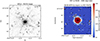 |
Fig. 1. Left panel: HST/WFC3 image of the central region obtained three years after the last outburst and with the F657N filter centered at the Hα emission line. This region is the same size as the MUSE-NFM of the T Pyx remnant. Right panel: Hα flux map reconstructed from the MUSE-NFM datacube. The black curves correspond to iso-surface brightness contours derived from the HST/WFC3 F657N image. The image scale is the same, but MUSE data were obtained 7.35 years (2685 days) after the HST data. This is reflected by the clear shift for the majority of the Hα-[N II] knots visible in the image. |
High-resolution spectroscopic observations several years post the explosion also show evidence for different types of aspherical ejecta (Chesneau et al. 2011; Shore et al. 2011, 2013; De Gennaro Aquino et al. 2014; Izzo 2015). Using HST-UV echelle observations of the nebular phase following the last outburst, Shore et al. (2013) explained the profiles observed in the main nebular emission lines with an axisymmetric bipolar geometry. However, our ignorance of the exact geometrical distribution of nova ejecta has an immediate effect on the estimate of the mass ejected in a nova outburst. The difference in the ejected mass inferred from the above models varies by one order of magnitude. This seems to be in agreement with the recent scenario proposed by Mukai & Sokoloski (2019), Aydi et al. (2020), where nova outbursts are characterized by two main ejection flows, each with different velocities, geometrical distributions, and origins, that interact and give rise to shocks during the brightest nova emission.
To shed light on the physical properties of the ejecta of T Pyx and on its possible role as one of the potential type-Ia SN progenitors in our Galaxy, we observed the remnant with new eyes, namely, with the Multi Unit Spectroscopic Explorer (MUSE) mounted at the UT4 (Yepun) of the European Southern Observatory (ESO) at the Cerro Paranal, Chile. In this work, we report on the analysis of the geometrical distribution of the remnant and the estimate of the distance to T Pyx using the nebular parallax method applied to the expanding ejecta from the last outburst in 2011. In Sect. 2, we describe the observations executed with MUSE, while in Sect. 3 we report on the analysis of the datacube obtained using the Wide Field Mode (WFM) and then on the extended remnant. In Sect. 4, we move to the analysis of the Narrow Field Mode (NFM), which allowed us to obtain a direct distance estimate to the system. In Sect. 5, we discuss our findings, and we draw our conclusions in Sect. 6.
2. Observations
The remnant of the RN T Pyx has been observed with MUSE (Bacon et al. 2010), which is mounted on the UT4 (Yepun) at the European Southern Observatory Very Large Telescope located in Paranal, Chile. MUSE is an integral field unit spectrograph capable of providing spatially resolved spectroscopy in the visible range. Two modes are available with MUSE: (1) a Wide Field Mode (WFM) that covers a region-wide 1 × 1 arcmin, with a nominal spatial sampling of 0.2 arcsec and a spectral resolution variable from R ∼ 1800 at 4800 Å and R ∼ 3600 at 9300 Å and (2) a Narrow Field Mode that allows for observations with a higher spatial resolution (sampling of 0.02 arcsec) in a narrower region of 7.5 × 7.5 arcsec but with a similar spectral resolution. With the WFM, the ground layer adaptive optics (GLAO) correction is used, which provides a correction of 0.2 × 0.2 arcsec over the entire field of view, while in NFM, the laser tomography adaptive optics (LTAO) is used, which provides a high correction with a diffraction core and a Strehl ratio between 5% and 10% at Hα. The use of adaptive optics, however, implies a gap in wavelengths of about ∼270 Å around the Na I D region (5890 Å) due to the use of the four sodium laser guide stars.
The NFM spatial resolution is comparable to that of HST images, but in addition to this, we also have the spectral information from each spaxel, which provided us with the radial velocity distribution from emission lines. This information can be used as a proxy for the “third” spatial dimension in order to reconstruct the 3D-geometric distribution of the explosion and obtain an accurate estimate of the distance. The NFM observations were done on November 15, 2021 (corresponding to 3868 days after the last outburst and to 2685 days, that is 7.35 years, after the HST observations reported in Fig. 1, which are considered as our reference for the nebular parallax analysis in Sect. 4). The WFM observations were performed on January 1 and 9, 2022 (see also Table 1). Data were reduced using the standard esorex recipes embedded in a single Python-based pipeline. After the creation of static calibration datacubes, namely bias, flat, and wavelength calibration, we also built the line-spread function and the illumination correction. Then, we applied the above corrections to the science and the standard datacubes and built the corresponding pixel tables for each single sensor. Finally, we obtained the response function for the standard star and obtained the final stacked science datacube. Astrometry was computed using HST archival data, with the central WD as the main reference. Sky emission residuals were subtracted using Zap (Soto et al. 2016) after masking all the sources in the field of view of MUSE-WFM whose emission is lower than the detection threshold of 1.5σ.
Diary of MUSE spectral observations.
3. The extended remnant
One of the great advantages of using IFU data consists of the possibility to reconstruct 2D images centered on a specific wavelength range and then, in the case of nova remnants, to focus on the emission from a given line feature. This allowed us to recover, for example, the emission from the hydrogen component alone, after subtracting the integrated flux in a given wavelength window region for the underlying stellar continuum of the central WD. In this way, 2D images of the expanding hydrogen ejecta were built from the WFM dataset by centering around the Hα (λ = 6562.8 Å) and Hβ (λ = 4861.3 Å) emission line, with an extraction wavelength window of Δλ = 20 Å. The final results show the presence of a tilted clumpy ring structure with an apparent semi-major radius of ≈5−6 arcsec (see Fig. 2). To model this component, we used the observed radial velocity as a proxy for the third spatial dimension z = vradt, given that at this epoch the ejecta is completely frozen and freely expanding. Using these flux maps and the distribution of the radial velocity of the gas along the hydrogen ring ejecta, we can determine the properties of the remnant such as the position angle PA and the inclination angle of the ring (see Fig. 3).
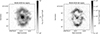 |
Fig. 2. Reconstructed Hα image of the remnant (left panel) and the corresponding Hβ image (right panel). Both images were obtained from the MUSE-WFM data as described in the main text. |
 |
Fig. 3. Modeling the spatial distribution of the T Pyx remnant. Left panel: three-dimensional reconstruction of the T Pyx remnant using the spatial resolution provided by the MUSE-WFM and using the radial velocity from the Hβ emission line as a proxy for the third dimension. The projection onto the corresponding 2D planes is shown with the gray data. Each single data point corresponds to a single bin resulting from the Voronoi tessellation algorithm described in Sect. 3. It is visible how the external remnant is arranged as a non-uniform thick ring, with inhomogeneities marked by the different flux intensities of the line (reported here with different colors). The line-of-sight direction is perpendicular to the X − Y (pixel–pixel) plane, and here it is shown as pointing to the top of the figure. Right panel: reference frame used to model the remnant of T Pyx and to recover the transformation equations described in Eq. (4), shown in black, with the observer’s line of sight located along the Z axis. The intrinsic remnant reference frame is reported with gray coordinates and a gray frame. The inclination (i) and position angle (PA) are also shown to help to reconstruct the projected model. |
However, due to the velocity distribution of the remnant, we could not estimate the de-projected radial velocity of the expanding gas using Hα because of the significant contamination from the nearby [N II] 6548/84 Å doublet. On the other hand, when focusing on the Hβ line, which is quite isolated from other contiguous bright emission lines such as [O III] 4959/5007 Å from the remnant and He II 4686 Å from the central WD, we were able to isolate the Hβ emission line and finally fit it with a Gaussian function. In this way, we could reconstruct the velocity field of the expanding ring structure without any contamination from other emission lines (see the right panel in Fig. 4). To perform this operation, we first re-binned the entire WFM datacube using a Voronoi tessellation algorithm previously masked for external field sources. This technique provided a spatially binned datacube based on the value of the signal-to-noise ratio in a specific wavelength region (Cappellari & Copin 2003). Since the Hβ line is fainter than Hα, we used the wavelength region centered on the Hα line with a width of δλ = 12.5 Å and a signal-to-noise threshold of 10. After this, we calculated the radial velocity of each spatial bin by fitting the Hβ emission line using a Gaussian function to measure the corresponding velocity offset after correcting for the barycentric velocity of T Pyx at the epoch of observations (vb = 16.5 km s−1). We masked the inner (r ≤ 5″) region while computing the radial velocity offset since it is dominated by the light from the central WD. The final Hβ radial velocity map of the remnant region outlined by the overplotted contours from the Hβ flux map presented in Fig. 2 is shown in Fig. 4.
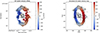 |
Fig. 4. Modeling the radial velocity of the T Pyx extended remnant. Left panel: Hβ radial velocity map obtained with the prescriptions given in the main text. The black curve represents the contour regions from the Hβ intensity flux map of Fig. 3. Right panel: simulated 2D radial velocity map of the ring remnant obtained from the best-fit parameters and the procedure delineated in the main text. |
To recover the geometric properties of the 3D ring remnant from the observed 2D map of Fig. 4, we initially simulated the three-dimensional geometry of the entire ring remnant for different values of the ring radius, expanding velocity, inclination, and position angle. To build our ring model, we used a Cartesian representation embedded within a python script developed for this analysis1. The initial 2D ring equation, which does not yet include any inclination along the observer’s line of sight, can be written as follows:
 (1)
(1)
where ϕ and θ are two angles modeling the ring and the width of its border and go over the (0, 360) deg range, R is the width of the ring, and r (fixed to 1 pixel) is the thickness of the ring border. When including tilt effects in our simulated ring, we took into account two other important parameters: (1) the inclination angle i, corresponding to the angle between the normal vector to the ring and the line of sight, and (2) the position angle PA, which takes into account any (anticlockwise) rotation of the tilted ring between the east direction in the sky and the ring radius connecting the ring center to the position of the observed “zero radial velocity”. This representation is very similar to the tilted disk model used to study galaxies and active galactic nuclei (Begeman 1989), with the only difference being that the gas is expanding radially in this case, while for galaxies the gas rotates.
Due to the symmetry of the model, there are two ring radii connecting the center to the zero velocity value, with the two radii lying in the same direction. To exclude any degeneracy, we fixed a prior on the position angle value that can vary between 0 and 180°. The inclusion of these two parameters provided us with the projected 2D equations, including the observed radial velocity value parameterized by the Z component:
 (2)
(2)
Here, to recover the intrinsic expanding velocity, we should correct v′ for the projected Z component, namely, vexp = v′*R/sin i. A graphical representation of our model is shown in Fig. 3, where the tilted ring parameters correspond to the best-fit values (see below).
Next, we had to compare our model with the observed 2D ring radial velocity distribution by projecting the resulting 3D ring geometry distribution onto the 2D spatial plane, corresponding to the observed image of the T Pyx remnant. The expanding velocity was assumed to be constant along the entire 3D distribution of the ring, which is a valid assumption for the frozen expanding gas at ∼10 years after the last outburst. Values of radial velocities were simulated for 180 data points along each projected ring (this was obtained by sampling the ϕ and θ angle parameters with a fixed separation between each pair of data of two degrees) and finally fitted to the observed radial velocity distribution. For this last operation, we performed the fit with a Markov chain Monte Carlo (MCMC) method using the emcee package (Foreman-Mackey et al. 2013). This MCMC methodology estimates the values of our unknown parameters by constructing a posterior distribution for all of them through the use of a likelihood function and a set of uniform priors for each of the parameters, which were first determined through an initial grid-search fit. Our Bayesian likelihood function is the classical chi-square function, with uncertainty values given by the observed radial velocity dispersion (obtained from the corresponding error datacube) for the relevant spatial bin of each observed data point.
The results of our MCMC fitting procedure are summarized in Fig. 5. We found that the remnant of T Pyx is best modeled by a ring structure with a radius of  arcsec, an expanding velocity of
  km s−1, an inclination angle of
  deg, and a position angle of PA =
  deg. Our results are in good agreement with the results obtained from the light echo analysis by Sokoloski et al. (2013). Moreover, we found a very good agreement with the position angle found using interferometric observations by Chesneau et al. (2011), Pavana et al. (2019) while taking into consideration that their analysis uses a bipolar ejecta geometry. Assuming a Gaia distance of 3.7 kpc (see above) and the expanding velocity determined above, we obtained an extension of the ring of Rphys = (2.76 ± 0.33)×1012 km, which would have been ejected tej = 207 ± 35 years ago by the central WD. This value would correspond to an eruption that happened in a relatively large time interval between 1779 and 1849. This result marginally agrees with the estimate by Schaefer et al. of a CN-like outburst of T Pyx in 1866 (Schaefer & Collazzi 2010), an estimate that nonetheless considered for T Pyx a slightly lower distance of 3.5 kpc. A larger distance of d = 4.8 ± 0.5 kpc, as recently proposed by Shore et al. (2013), Sokoloski et al. (2013) would only agree within 2σ with the estimation of Schaefer & Collazzi (2010), resulting in a CN-like ejection epoch that happened tej = 270 ± 56 years ago. T Pyx should be at a closer distance to be in full agreement with the Schaefer & Collazzi (2010) calculation. An accurate distance of T Pyx can shed light on the origin of the ring structure. We remark that we have not considered any deceleration of the ejecta due to the snowplow effect from interaction with the surrounding CSM or with gas from previous eruptions. An extended remnant initially expanding at larger velocities would suggest a more recent CN-like eruption and then agree with Schaefer & Collazzi (2010). A more detailed analysis of the extended remnant will be presented in a future publication.
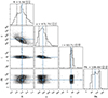 |
Fig. 5. Posterior distribution and corner plots obtained from the MCMC fitting procedure described in Sect. 3. |
4. The 2011 outburst ejecta
The possibility of combining the spectral information of spatially identified structures allowed us to obtain an accurate measurement of the distance to T Pyx using the nebular parallax method (Baade 1940; Cohen 1985; Krautter et al. 2002). The remnant of T Pyx has been observed a few times with HST after the last outburst of 2011 (Toraskar et al. 2013; Godon et al. 2014; Shara et al. 2015). In one of the most recent observations, a bipolar ejecta was clearly identified along the WE direction, in particular when using the narrow filters F657N available with the Wide Field Camera (HST GO program ID: 13796, PI: Crotts; see also Fig. 1). We searched for the presence of evidence of this bipolar structure in the MUSE-NFM datacube, which has a very high spatial resolution of ∼0.03 arcsec, comparable to the HST/WFC3 resolution. First, we studied the reconstructed Hα map and detected all the knots observed by HST in 2014. For the majority of them, we also noticed a shift in the spatial coordinates due to their expanding motion. We also identified an extended knot in the W direction with respect to the central WD that is absent in pre-2011 outburst HST images and has been confirmed to be the expanding outflow of the 2011 outburst only thanks to the reconstruction of the [O III] map. Indeed, late nebular spectra of the 2011 outburst of T Pyx have shown the presence of bright [O III] lines a few years after the initial explosion of the nova (Shore et al. 2013; Pavana et al. 2019). Unlike the Hα line, the wavelength region surrounding the [O III] λλ4959/5007 doublet is far from the bright lines observed in emission from the central WD and its accretion disk (He I 4922 and 5016 Å lines are visible only in the innermost regions where light from the central WD dominates). The [O III] emission line map covering a region of ∼2 arcmin radius from the central WD is shown in Fig. 6.
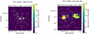 |
Fig. 6. The 2011 outburst ejecta observed with MUSE-NFM. Left panel: the [O III] gas distribution observed with the MUSE-NFM (7.5″ × 7.5″). White contours correspond to iso-surface brightness contours derived from the HST/WFC3 F657N image. Right panel: two 2″ × 2″ zoom-ins of the region covering the central WD and the bright pole ejecta. After registering the MUSE [O III] map for the HST astrometry, we measured a shift of 0.71 arcsec between the centroid positions of the ejecta observed in 2014 (with HST – green cross) and in 2021 (with MUSE – red cross). |
The resulting [O III] map clearly shows the presence of two extended structures at larger, and opposite, distances from the central WD if compared to the HST observation made 7.35 years before the MUSE observations. The western lobe turns out to be brighter than the eastern one, and it also shows some sub-structures, suggesting a complex shape for the ejected mass. The integrated spectra of both blobs, extracted from the MUSE-NFM dataset and subtracted from the underlying residual WD emission using a background region with the same pixel area as the source extraction region, shows that the western lobe is blueshifted (vrad = −798 ± 50 km s−1) with respect to the eastern counterpart (see Fig. 7). Interestingly, the Hβ line shows only the component from the underlying WD and is located at the systemic velocity of T Pyx. A faint residual emission is visible at bluer wavelengths with the same blueshift reported for the western blob. This evidence explains the fainter emission from the eastern lobe as being more distant and then passing through a thicker circumstellar medium, and it also confirms that the bipolar ejecta are directed toward the perpendicular direction to the plane of the larger ring-like structure, which was characterized previously using the MUSE-WFM dataset (see Sect. 3). This characteristic allowed us to use the information obtained for the spatial orientation of the ring-like structure to determine the velocity component of the bipolar ejecta tangential to the line of sight. Then, we could use the yearly parallax of the bipolar ejecta, after determining the separation between the western blob observed in the HST image of 2014 and the MUSE/NFM 2021 datacube, with the information on the tangential velocity to determine the distance using the nebular parallax method.
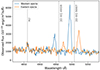 |
Fig. 7. Wavelength region between 4800 and 5100 Å of the western blob ejecta (blue data) and the eastern blob (orange data) detected in the MUSE-NFM dataset. The dashed gray lines mark the rest-frame wavelength for the Hβ and the [O III] 4959/5007 lines. While Hβ is mainly detected at a zero velocity offset, suggesting it mainly comes from the gas surrounding the progenitor WD, [O III] lines show a radial velocity offset originating from the ejecta of the 2011 outburst. |
A more detailed insight on the [O III] map also shows the presence of a structure in the western blob ejecta. While the HST image shows a compact spheroidal knot, the NFM data reveal the presence of two elongated filaments that spread laterally to the main compact ejecta. We noticed that a similar structure was already inferred in 1D spectral analyses (Shore et al. 2013; Pavana et al. 2019). To determine the position of the western blob in both datasets, we first determined the centroids of the blue ejecta from the HST/WFC3 image and the MUSE-NFM [O III] map, after being corrected for the HST astrometry. For the exact measurement of the centroids, we used the centroid_com package, available within the photutils Python package (Bradley et al. 2022). In particular, we first selected the region of the HST and MUSE-NFM [O III] maps (after being registered for the astrometry of the HST-WFC3 image) containing the western blob, and then we calculated the centroids of the corresponding observed light distribution by estimating the center of mass determined from moments of the light distribution. Finally, we reconverted the centroid values into World Coordinate System (WCS) coordinates using the astrometry of the HST image. The centroids of the western blob in the two epochs are reported in Table 2, while the results of our analysis are shown in Fig. 6. The resulting distance of the two centroids amounts to d = 0.69 ± 0.04 (stat.)±0.05 (sys.) arcsec.
Centroid positions (in image and WCS J2000.0 coordinates) of the western blobs in the HST and MUSE-NFM maps.
The computed centroids of the western blob at both epochs display a tilt of ϕ = 5.3 deg with respect to the WE direction. Assuming that the direction of this ejecta component is normal to the plane of the ring distribution derived in Sect. 3, this value is in agreement within 1σ with the position angle value found in the previous analysis (see Sect. 3). This hypothesis is also supported by the evidence that the western blob displays a blueshifted, and larger, radial velocity, while the western ring component shows redshifted and lower velocity values. This evidence also supports the proposal of a multicomponent ejection in T Pyx. However, we did not find clear evidence of a ring component from the 2011 outburst nor from previous outbursts. This can mainly be attributed to two factors: (1) low spatial resolution of the available dataset, which prevents us from disentangling the ring from the nearby bright WD, and (2) the possibility that the ring component is not massive enough to emit hydrogen spectral lines detectable with MUSE. Another possibility, which nonetheless needs more investigation, is that the more recent T Pyx outbursts only displayed a bipolar ejecta, while the massive ring component was produced in a more energetic explosion that happened farther back in time. Indeed, detailed nebular analyses have excluded the presence of continuous wind in the last outburst, and the best model that fits the observed line structure is provided by an axial bipolar symmetry (Shore et al. 2013; De Gennaro Aquino et al. 2014). A complete physical characterization in terms of ejecta constitution and abundance of the extended remnant will be studied in a forthcoming publication.
5. Discussion
Characterization of the geometry distribution of the remnant of T Pyx paves the way to determining the distance to the nova using the nebular parallax method (Baade 1940; Cohen 1985; Krautter et al. 2002). We determined the tangential offset displayed by the ejecta of 2011 as observed in two epochs separated by 7.35 years, but we still needed information about the tangential velocity of the ejecta itself. This can be determined using the MUSE spectrum of the western blob, in particular through the measurement of the radial velocity from emission lines such as [O III], and then transforming this into a tangential velocity value using the geometry of the remnant determined previously. The spectra of the bipolar ejecta both show a radial velocity offset of vr, ej = 798 ± 50 km s−1 (corrected for the measured systemic velocity of vsys = +28 km s−1), which is opposite in sign for the eastern blob (see also Fig. 7). According to the assumed geometrical representation (see also Fig. 3), we can determine the tangential velocity by correcting the observed radial velocity of the ejecta for the position (PA) and the inclination angle (i) through vt, ej = vr, ej × tani. Using the results derived in Sect. 3, we obtained a tangential velocity of vt, ej = 1613 ± 340 km s−1. At this point, we had all the ingredients to derive the nebular parallax distance, which is defined by
 (3)
(3)
where  arcsec yr−1 is the estimated expansion parallax and vt, ej is given in kilometers per second (Wade 1990; Duerbeck 1992). This distance value is in full agreement with the previous distance estimates existing in the literature for T Pyx (Selvelli et al. 2008; Schaefer & Collazzi 2010) and with the Gaia measurement (Gaia Collaboration 2021), but it is only marginally consistent with the value given in Shore et al. (2011), Sokoloski et al. (2013).
With the knowledge of the distance to T Pyx, thanks to the geometrical reconstruction of the bipolar ejecta, and its size, it was also possible to provide an estimate of the mass of the bipolar ejecta using the information available in the western blob spectrum alone, assuming that the same mass is expelled in both directions. A widely used methodology to infer nova ejecta masses from nebular phase spectra consists of measuring electron temperatures and accurate fluxes for Balmer lines (in this case we considered the Hβ line, given that the Hα is strongly blended with [N II]) so that one can directly determine the electron density in the ejecta as well as the ejected mass based on the exact knowledge of the ejecta volume (Mustel & Boyarchuk 1970). To state briefly, the luminosity of the Hβ line can be expressed by
 (4)
(4)
where ϵHβ is the emission coefficient for Hβ at the temperature of T = 10 000 K, which is typical of case B recombination (Osterbrock & Ferland 2006); ne is the electron density, assumed to be equal to the hydrogen density (np = ne); and V is the volume of the ejecta. A drawback of this methodology is its lack of precise geometrical characterization of the ejecta itself, for which a general assumption of a spherical shell, corrected for the filling factor of the gas, is usually considered (see e.g. Della Valle et al. 2002; Mason et al. 2005). In the case of T Pyx, we have a direct measurement of the size of the western bipolar ejecta, assuming it is best characterized by a structured spherical blob with rej = 0.22 arcsec, which at the distance of d = 3.55 ± 0.77 kpc results in a volume of V = (5.43 ± 0.90)×1048 cm3. However, we cannot exclude the clumpiness of the ejecta (Santamaría et al. 2022), as can be deduced from the [O III] map in Fig. 6, which would still give rise to a multiplicative filling factor term. Here, we assume a conservative value of f ≂ 0.1 for the filling factor, whereas Shore et al. (2013) found f = 0.03 (but using integrated 1D spectra).
The spectrum extracted from the western blob does not show any clear evidence for Hβ at the same radial velocity of [O III] lines, which is the main signature of hydrogen emission from the ejecta. Assuming the same FWZI reported for the [O III] line, we measured a de-reddened (with E(B − V) = 0.25 mag, Gilmozzi & Selvelli 2007) upper limit of F(Hβ) < 4.5 × 10⁻¹⁷ erg cm−2 s−1, which corresponds to a luminosity of L(Hβ) < 6.7 × 1029 erg s−1 at the distance of d = 3.55 ± 0.77 kpc. Interestingly, emission due to Hβ from the central WD was clearly detected (see also Figs. 7 and 8), whose origin is likely due to gas surrounding the progenitor system. We could then determine the mass of the western blob using the following formula:
 (5)
(5)
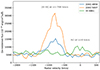 |
Fig. 8. Spectrum of the western blob expressed in radial velocity with the wavelength centered on [O III] 4959 Å (blue data), 5007 Å (orange), and Hβ (green). We note the absence of emission from Hβ at the blueshift velocity value where emission from [O III] is detected. The Hβ emission was, however, detected at zero radial velocity, and its origin likely comes from the gas surrounding the progenitor WD (work in preparation). |
under the assumption that ne = np = 315.7 ± 56.4 cm−3, as determined from Eq. (4), and with mp being the proton mass. We obtained an upper limit for the bipolar ejecta of Mej, b < (3.0 ± 1.0)×10−6 M⊙. This estimate does not include any effect of the filling factor due to clumpiness or structured ejecta, suggesting that the upper limit could also be lower by up to one order of magnitude.
We immediately noticed that despite being an upper limit, this value is lower than any measurements reported so far in the literature for the 2011 outburst. Optical studies have reported ejecta masses ranging from Mej = 7 × 10⁻⁶ M⊙ (Pavana et al. 2019) to Mej = 2 × 10⁻⁵ M⊙ (Shore et al. 2013), while we have similar values at other wavelengths from X-ray analysis, Mej ≈ 10−5 M⊙ (Chomiuk et al. 2014), and possibly more significant ejecta using radio observations, Mej = 1−30 × 10−5 M⊙ (Nelson et al. 2014). However, the analysis of the variation of the orbital period before and after the 2011 outburst also suggests a greater ejecta value, Mej = 2 × 10⁻⁵ M⊙ (Patterson et al. 2017). We note that for the distance of d = 4.8 ± 0.5 kpc (Sokoloski et al. 2013), the upper limit for the mass of the bipolar ejecta is Mej, b, S13 < (6.8 ± 2.0)×10−6 M⊙, a value that is consistent with the estimate given in Pavana et al. (2019). We also emphasize that this upper limit applies only to the bipolar ejecta identified in the MUSE-NFM observations and that it does not take into account the presence of a slower ring component, whose lack of clear evidence in the MUSE-NFM data prevented us from quantifying its contribution to the global ejected mass. A more detailed analysis is still needed, and this will be the topic of a forthcoming publication dedicated to the extended remnant of T Pyx.
6. Conclusions
In this work we have presented a study of the geometrical distribution of the gas surrounding the recurrent nova T Pyx as observed by the ESO/MUSE IFU detector. Notably, MUSE allowed us to perform a spatially resolved study of the spectral emission from the extended remnant, using the WFM configuration, and the more internal (field of view was 7.5 × 7.5 arcsec2) regions surrounding the progenitor WD, with an incredible spatial sampling of 0.02 arcsec. The results of our analysis are summarized as follows:
-
The reconstructed Balmer emission line image using the MUSE-WFM datacube shows the presence of a tilted ring (see Fig. 4). The ring shows blueshifted radial velocities on the eastern side and redshifted values on the western side, suggesting the existence of an equatorial ejecta component that has shaped the extended remnant.
-
We modeled the reconstructed Hβ remnant emission using a formalism typically used in the study of tilted disks in galaxies and active galactic nuclei (Begeman 1989) but with a radially expanding velocity for the gas, instead of the generic rotating formalism (see Figs. 1 and 3). We measured the inclination of the remnant along our line of sight to be
 deg, while the remnant extension has a radius of
  arcsec, with the ejecta having an expanding velocity of
  km s−1.
 -
The MUSE-NFM dataset shows the presence of a bipolar outflow characterized by opposite expanding velocities when compared to the extended ring remnant: blueshifted velocities were observed on the western ejecta and redshifted values on the eastern one. This evidence implies the existence of a bipolar outflow, which has also been observed in HST images obtained three years after the last outburst but not before, pointing out that this bipolar outflow originated in the 2011 outburst of T Pyx.
-
The MUSE-NFM analysis revealed an offset of the Western blob of r = 0.69 ± 0.04 (stat.)±0.05 (sys.) arcsec (see Fig. 6), which corresponds to an expansion parallax of
 arcsec yr−1, using the 2014 HST image as a reference. With these values, we determined a nebular parallax distance to T Pyx of d = 3.55 ± 0.77 kpc.
 -
With the knowledge of the distance and the lack of a detected Hβ emission line (see Fig. 8), we first estimated the volume of the western blob and then set an upper limit to the bipolar ejected mass, assuming case B recombination physical conditions for the gas in the ejecta. We obtained an upper limit of Mej, b < (3.0 ± 1.0)×10−6 M⊙ for the bipolar ejecta in T Pyx, a value that does not include any correction for the ejecta filling factor. Including this correction, we obtained a mass limit that is lower than the total accreted mass on the primary WD during the quiescence phase between the last two recent outbursts of T Pyx (Selvelli et al. 2008; Godon et al. 2014; Patterson et al. 2017).
In a forthcoming paper, we will discuss in more detail the physical properties of the extended remnant. Our focus will be on examining the impact of multiple outbursts in shaping the observed gas distribution in order to facilitate a comparison between the material accreted between outbursts and the average mass of the ejecta.
Acknowledgments
L.I. was supported by a VILLUM FONDEN Investigator grant (project number 16599). E.A. acknowledges support by NASA through the NASA Hubble Fellowship grant HST-HF2-51501.001-A awarded by the Space Telescope Science Institute, which is operated by the Association of Universities for Research in Astronomy, Inc., for NASA, under contract NAS5-26555. M.O.H. was supported by the Polish National Science Centre grant 2019/32/C/ST9/00577. Data Availability: The MUSE datacubes are available upon reasonable request. We uploaded the datacubes and the codes used for the modeling of the remnant of T Pyx to a dedicated GitHub repository, which is reported in the manuscript.
References
- Aydi, E., Chomiuk, L., Izzo, L., et al. 2020, ApJ, 905, 62 [NASA ADS] [CrossRef] [Google Scholar]
- Baade, W. 1940, PASP, 52, 386 [CrossRef] [Google Scholar]
- Bacon, R., Accardo, M., Adjali, L., et al. 2010, in Ground-based and Airborne Instrumentation for Astronomy III, eds. I. S. McLean, S. K. Ramsay, & H. Takami, SPIE Conf. Ser., 7735, 773508 [Google Scholar]
- Bailer-Jones, C. A. L. 2015, PASP, 127, 994 [Google Scholar]
- Bailer-Jones, C. A. L., Rybizki, J., Fouesneau, M., Mantelet, G., & Andrae, R. 2018, AJ, 156, 58 [Google Scholar]
- Begeman, K. G. 1989, A&A, 223, 47 [NASA ADS] [Google Scholar]
- Bode, M. F., & Evans, A. 2008, Classical Novae (Cambridge: Cambridge University Press) [CrossRef] [Google Scholar]
- Bradley, L., Sipőcz, B., Robitaille, T., et al. 2022, https://doi.org/10.5281/zenodo.7419741 [Google Scholar]
- Cappellari, M., & Copin, Y. 2003, MNRAS, 342, 345 [Google Scholar]
- Chesneau, O., Meilland, A., Banerjee, D. P. K., et al. 2011, A&A, 534, L11 [NASA ADS] [CrossRef] [EDP Sciences] [Google Scholar]
- Chomiuk, L., Nelson, T., Mukai, K., et al. 2014, ApJ, 788, 130 [NASA ADS] [CrossRef] [Google Scholar]
- Cohen, J. G. 1985, ApJ, 292, 90 [CrossRef] [Google Scholar]
- De Gennaro Aquino, I., Shore, S. N., Schwarz, G. J., et al. 2014, A&A, 562, A28 [NASA ADS] [CrossRef] [EDP Sciences] [Google Scholar]
- Della Valle, M., & Izzo, L. 2020, A&ARv, 28, 3 [NASA ADS] [CrossRef] [Google Scholar]
- Della Valle, M., & Livio, M. 1996, ApJ, 473, 240 [NASA ADS] [CrossRef] [Google Scholar]
- Della Valle, M., Pasquini, L., Daou, D., & Williams, R. E. 2002, A&A, 390, 155 [NASA ADS] [CrossRef] [EDP Sciences] [Google Scholar]
- Duerbeck, H. W. 1992, Acta Astron., 42, 85 [NASA ADS] [Google Scholar]
- Duerbeck, H. W., & Seitter, W. C. 1979, The Messenger, 17, 1 [NASA ADS] [Google Scholar]
- Foreman-Mackey, D., Hogg, D. W., Lang, D., & Goodman, J. 2013, PASP, 125, 306 [Google Scholar]
- Gaia Collaboration (Brown, A. G. A., et al.) 2021, A&A, 649, A1 [NASA ADS] [CrossRef] [EDP Sciences] [Google Scholar]
- Gallagher, J. S., & Starrfield, S. 1978, ARA&A, 16, 171 [NASA ADS] [CrossRef] [Google Scholar]
- Gilmozzi, R., & Selvelli, P. 2007, A&A, 461, 593 [NASA ADS] [CrossRef] [EDP Sciences] [Google Scholar]
- Godon, P., Sion, E. M., Starrfield, S., et al. 2014, ApJ, 784, L33 [NASA ADS] [CrossRef] [Google Scholar]
- Izzo, L., della Valle, M., Ederoclite, A., & Henze, M. 2015, Acta Polytech. CTU Proc., 2, 264 [CrossRef] [Google Scholar]
- Joshi, V., Banerjee, D. P. K., & Ashok, N. M. 2014, MNRAS, 443, 559 [NASA ADS] [CrossRef] [Google Scholar]
- Krautter, J., Woodward, C. E., Schuster, M. T., et al. 2002, AJ, 124, 2888 [CrossRef] [Google Scholar]
- Mason, E., Della Valle, M., Gilmozzi, R., Lo Curto, G., & Williams, R. E. 2005, A&A, 435, 1031 [NASA ADS] [CrossRef] [EDP Sciences] [Google Scholar]
- Mukai, K., & Sokoloski, J. L. 2019, Phys. Today, 72, 38 [NASA ADS] [CrossRef] [Google Scholar]
- Mustel, E. R., & Boyarchuk, A. A. 1970, Ap&SS, 6, 183 [NASA ADS] [CrossRef] [Google Scholar]
- Nelson, T., Chomiuk, L., Roy, N., et al. 2014, ApJ, 785, 78 [CrossRef] [Google Scholar]
- Nomoto, K., Thielemann, F. K., & Yokoi, K. 1984, ApJ, 286, 644 [Google Scholar]
- Osterbrock, D. E., & Ferland, G. J. 2006, Astrophysics of Gaseous Nebulae and Active Galactic Nuclei (Sausalito: University Science Books) [Google Scholar]
- Patterson, J., Oksanen, A., Kemp, J., et al. 2017, MNRAS, 466, 581 [CrossRef] [Google Scholar]
- Pavana, M., Anche, R. M., Anupama, G. C., Ramaprakash, A. N., & Selvakumar, G. 2019, A&A, 622, A126 [NASA ADS] [CrossRef] [EDP Sciences] [Google Scholar]
- Santamaría, E., Guerrero, M. A., Toalá, J. A., Ramos-Larios, G., & Sabin, L. 2022, MNRAS, 517, 2567 [CrossRef] [Google Scholar]
- Schaefer, B. E., & Collazzi, A. C. 2010, AJ, 139, 1831 [CrossRef] [Google Scholar]
- Selvelli, P., Cassatella, A., Gilmozzi, R., & González-Riestra, R. 2008, A&A, 492, 787 [NASA ADS] [CrossRef] [EDP Sciences] [Google Scholar]
- Shafter, A. W., Henze, M., Rector, T. A., et al. 2015, ApJS, 216, 34 [NASA ADS] [CrossRef] [Google Scholar]
- Shara, M. M., Moffat, A. F. J., Williams, R. E., & Cohen, J. G. 1989, ApJ, 337, 720 [NASA ADS] [CrossRef] [Google Scholar]
- Shara, M. M., Zurek, D. R., Williams, R. E., et al. 1997, AJ, 114, 258 [NASA ADS] [CrossRef] [Google Scholar]
- Shara, M. M., Zurek, D., Schaefer, B. E., et al. 2015, ApJ, 805, 148 [NASA ADS] [CrossRef] [Google Scholar]
- Shore, S. N., Augusteijn, T., Ederoclite, A., & Uthas, H. 2011, A&A, 533, L8 [NASA ADS] [CrossRef] [EDP Sciences] [Google Scholar]
- Shore, S. N., Schwarz, G. J., De Gennaro Aquino, I., et al. 2013, A&A, 549, A140 [NASA ADS] [CrossRef] [EDP Sciences] [Google Scholar]
- Sokoloski, J. L., Crotts, A. P. S., Lawrence, S., & Uthas, H. 2013, ApJ, 770, L33 [NASA ADS] [CrossRef] [Google Scholar]
- Soto, K. T., Lilly, S. J., Bacon, R., Richard, J., & Conseil, S. 2016, MNRAS, 458, 3210 [Google Scholar]
- Starrfield, S., Sparks, W. M., & Truran, J. W. 1985, ApJ, 291, 136 [CrossRef] [Google Scholar]
- Starrfield, S., Iliadis, C., & Hix, W. R. 2016, PASP, 128, 051001 [Google Scholar]
- Surina, F., Hounsell, R. A., Bode, M. F., et al. 2014, AJ, 147, 107 [NASA ADS] [CrossRef] [Google Scholar]
- Toraskar, J., Mac Low, M.-M., Shara, M. M., & Zurek, D. R. 2013, ApJ, 768, 48 [NASA ADS] [CrossRef] [Google Scholar]
- Uthas, H., Knigge, C., & Steeghs, D. 2010, MNRAS, 409, 237 [NASA ADS] [CrossRef] [Google Scholar]
- Wade, R. A. 1990, in IAU Colloq. 122: Physics of Classical Novae, eds. A. Cassatella, & R. Viotti, 369, 179 [NASA ADS] [CrossRef] [Google Scholar]
- Warner, B. 1973, MNRAS, 162, 189 [NASA ADS] [Google Scholar]
- Webbink, R. F., Livio, M., Truran, J. W., & Orio, M. 1987, ApJ, 314, 653 [NASA ADS] [CrossRef] [Google Scholar]
- Whelan, J., & Iben, I., Jr. 1973, ApJ, 186, 1007 [Google Scholar]
- Williams, R. E. 1982, ApJ, 261, 170 [NASA ADS] [CrossRef] [Google Scholar]
All Tables
Centroid positions (in image and WCS J2000.0 coordinates) of the western blobs in the HST and MUSE-NFM maps.
All Figures
|
Fig. 1. Left panel: HST/WFC3 image of the central region obtained three years after the last outburst and with the F657N filter centered at the Hα emission line. This region is the same size as the MUSE-NFM of the T Pyx remnant. Right panel: Hα flux map reconstructed from the MUSE-NFM datacube. The black curves correspond to iso-surface brightness contours derived from the HST/WFC3 F657N image. The image scale is the same, but MUSE data were obtained 7.35 years (2685 days) after the HST data. This is reflected by the clear shift for the majority of the Hα-[N II] knots visible in the image. |
| In the text | |
|
Fig. 2. Reconstructed Hα image of the remnant (left panel) and the corresponding Hβ image (right panel). Both images were obtained from the MUSE-WFM data as described in the main text. |
| In the text | |
|
Fig. 3. Modeling the spatial distribution of the T Pyx remnant. Left panel: three-dimensional reconstruction of the T Pyx remnant using the spatial resolution provided by the MUSE-WFM and using the radial velocity from the Hβ emission line as a proxy for the third dimension. The projection onto the corresponding 2D planes is shown with the gray data. Each single data point corresponds to a single bin resulting from the Voronoi tessellation algorithm described in Sect. 3. It is visible how the external remnant is arranged as a non-uniform thick ring, with inhomogeneities marked by the different flux intensities of the line (reported here with different colors). The line-of-sight direction is perpendicular to the X − Y (pixel–pixel) plane, and here it is shown as pointing to the top of the figure. Right panel: reference frame used to model the remnant of T Pyx and to recover the transformation equations described in Eq. (4), shown in black, with the observer’s line of sight located along the Z axis. The intrinsic remnant reference frame is reported with gray coordinates and a gray frame. The inclination (i) and position angle (PA) are also shown to help to reconstruct the projected model. |
| In the text | |
|
Fig. 4. Modeling the radial velocity of the T Pyx extended remnant. Left panel: Hβ radial velocity map obtained with the prescriptions given in the main text. The black curve represents the contour regions from the Hβ intensity flux map of Fig. 3. Right panel: simulated 2D radial velocity map of the ring remnant obtained from the best-fit parameters and the procedure delineated in the main text. |
| In the text | |
|
Fig. 5. Posterior distribution and corner plots obtained from the MCMC fitting procedure described in Sect. 3. |
| In the text | |
|
Fig. 6. The 2011 outburst ejecta observed with MUSE-NFM. Left panel: the [O III] gas distribution observed with the MUSE-NFM (7.5″ × 7.5″). White contours correspond to iso-surface brightness contours derived from the HST/WFC3 F657N image. Right panel: two 2″ × 2″ zoom-ins of the region covering the central WD and the bright pole ejecta. After registering the MUSE [O III] map for the HST astrometry, we measured a shift of 0.71 arcsec between the centroid positions of the ejecta observed in 2014 (with HST – green cross) and in 2021 (with MUSE – red cross). |
| In the text | |
|
Fig. 7. Wavelength region between 4800 and 5100 Å of the western blob ejecta (blue data) and the eastern blob (orange data) detected in the MUSE-NFM dataset. The dashed gray lines mark the rest-frame wavelength for the Hβ and the [O III] 4959/5007 lines. While Hβ is mainly detected at a zero velocity offset, suggesting it mainly comes from the gas surrounding the progenitor WD, [O III] lines show a radial velocity offset originating from the ejecta of the 2011 outburst. |
| In the text | |
|
Fig. 8. Spectrum of the western blob expressed in radial velocity with the wavelength centered on [O III] 4959 Å (blue data), 5007 Å (orange), and Hβ (green). We note the absence of emission from Hβ at the blueshift velocity value where emission from [O III] is detected. The Hβ emission was, however, detected at zero radial velocity, and its origin likely comes from the gas surrounding the progenitor WD (work in preparation). |
| In the text | |
Current usage metrics show cumulative count of Article Views (full-text article views including HTML views, PDF and ePub downloads, according to the available data) and Abstracts Views on Vision4Press platform.
Data correspond to usage on the plateform after 2015. The current usage metrics is available 48-96 hours after online publication and is updated daily on week days.
Initial download of the metrics may take a while.