| Issue |
A&A
Volume 686, June 2024
|
|
|---|---|---|
| Article Number | A247 | |
| Number of page(s) | 12 | |
| Section | Extragalactic astronomy | |
| DOI | https://doi.org/10.1051/0004-6361/202348587 | |
| Published online | 17 June 2024 | |
A MUSE view of the core of the giant low-surface-brightness galaxy Malin 1
1
Instituto de Estudios Astrofísicos, Facultad de Ingeniería y Ciencias, Universidad Diego Portales, Av. Ejército Libertador 441, Santiago, Chile
e-mail: This email address is being protected from spambots. You need JavaScript enabled to view it.
2
Instituto de Astrofísica, Pontificia Universidad Católica de Chile, Av. Vicuña Mackenna 4860, 7820436 Macul, Santiago, Chile
3
Instituto de Alta Investigación, Universidad de Tarapacá, Casilla 7D, Arica, Chile
4
Aix Marseille Univ., CNRS, CNES, LAM, Marseille, France
5
Canada-France-Hawaii Telescope, 65-1238 Mamalahoa Highway, Kamuela, HI 96743, USA
6
National Centre for Nuclear Research, Pasteura 7, 02-093 Warsaw, Poland
7
Leibniz-Institut für Astrophysik Potsdam (AIP), An der Sternwarte 16, 14482 Potsdam, Germany
Received:
13
November
2023
Accepted:
5
April
2024
Abstract
Aims. The central region of the giant low-surface-brightness galaxy Malin 1 has long been known to have a complex morphology, with evidence of a bulge, disc, and potentially a bar hosting asymmetric star formation. In this work, we use VLT/MUSE data to resolve the central region of Malin 1 in order to determine its structure.
Methods. We used careful light profile fitting in every image slice of the datacube to create wavelength-dependent models of each morphological component, from which we were able to cleanly extract their spectra. We then used the kinematics and emission line properties from these spectra to better understand the nature of each component extracted from our model fitting.
Results. We report the detection of a pair of distinct sources at the centre of this galaxy with a separation of ∼1.05″, which corresponds to a separation on sky of ∼1.9 kpc. The radial velocity data of each object confirm that they both lie in the kinematic core of the galaxy. An analysis of the emission lines reveals that the central compact source is more consistent with being ionised through star formation and/or a LINER, while the off-centre compact source lies closer to the separation between star-forming galaxies and active galactic nuclei.
Conclusions. This evidence suggests that the centre of Malin 1 hosts either a bar with asymmetric star formation or two distinct components. In the latter scenario, we propose two hypotheses for the nature of the off-centre compact source-it could either be a star-forming clump, containing one or more star clusters, that is in the process of falling into the core of the galaxy and eventually merging with the central nuclear star cluster, or it could be a clump of gas falling into the centre of the galaxy from either outside or from the disc and triggering star formation there.
Key words: galaxies: elliptical and lenticular / cD / galaxies: individual: Malin 1 / galaxies: star clusters: general
© The Authors 2024
 Open Access article, published by EDP Sciences, under the terms of the Creative Commons Attribution License (https://creativecommons.org/licenses/by/4.0), which permits unrestricted use, distribution, and reproduction in any medium, provided the original work is properly cited.
This article is published in open access under the Subscribe to Open model. This email address is being protected from spambots. You need JavaScript enabled to view it. to support open access publication.
1. Introduction
Since its discovery (Bothun et al. 1987), Malin 1 has always been an unusual member of the class of giant low-surface-brightness (GLSB) galaxies. It has very faint disk with a surface brightness of ∼28 mag arcsec−2 in the B-band and an extraordinary size of ∼200 kpc (Moore & Parker 2006; Galaz et al. 2015; Boissier et al. 2016), possibly making it the largest single spiral observed to date. But it also reveals perplexing features, including a large reservoir of ∼6 × 10¹⁰ M⊙ of HI (Pickering et al. 1997), and no direct evidence of molecular gas to date (Braine et al. 2000; Das et al. 2010; Galaz et al. 2022). On the other hand, the inner region, of radius of ∼10 kpc, resembles a typical SB0/a galaxy (Barth 2007). This inner region is also complex, with evidence of a bulge+disc+bar morphology (Barth 2007; Junais et al. 2020; Saha et al. 2021) and emission line properties indicating the presence of both star formation (Junais et al. 2020; Saha et al. 2021) and LINER activity (Barth 2007; Subramanian et al. 2016; Junais et al. 2020).
A recent study of Malin 1 by Saha et al. (2021) has also revealed that when zoomed in, the central bar structure can be resolved into two clumps that resemble a bar-like structure in far-ultaviolet (FUV) images of the galaxy; however their Fig. 5 shows that the FUV emission appears to be misaligned with respect to the bar. From their observations in the UV and of strong emission lines, they conclude that this region has undergone recent star formation (< 10 Myr), and hosts hot blue stars, despite their measurements of the Hα and FUV star formation rates (SFRs) within the central 3″ being low enough that the galaxy would normally be considered quenched. If these two clumps at the core of Malin 1 were to be confirmed (both photometrically and kinematically) as distinct, they may reflect a rare and challenging example of a the growth of a nuclear star cluster (NSC) through the merging and accretion of infalling gas or star clusters.
NSCs are a common characteristic of galaxies of all masses and morphologies, with a recent study of spiral galaxies by Ashok et al. (2023) finding 80% of the sample hosted NSCs, but their formation and mass assembly processes are still uncertain. Two main scenarios have been proposed to explain the formation of NSCs. The first process is the in situ scenario, in which the NSC is formed in the central few parsecs of the galaxy through star formation fuelled by infalling gas (Milosavljević 2004; Bekki et al. 2006; Bekki 2007). In this scenario, the star formation timescale and occurrences of later star formation are dependent on the gas reservoirs within the galaxy. The second scenario is the migration scenario, in which a globular cluster (GC) forms within the galaxy and migrates to the centre of the galaxy via dynamical friction (Tremaine et al. 1975). Thus, NSCs created in this way can build up their mass at later times through mergers with other infalling GCs (Andersen et al. 2008). As dynamical friction is most efficient between systems with similar velocity dispersion, this process is thought to be most active in dwarf galaxies (e.g. Lotz et al. 2001; Miller & Lotz 2007; Neumayer et al. 2020; Fahrion et al. 2021).
In reality however, it is unlikely that one single process dominates the formation of NSCs. Consequently, a hybrid scenario has been suggested, the “wet-migration” scenario (Guillard et al. 2016). In this case, a GC forms with its own gas reservoir somewhere in the disc of the galaxy. As the GC migrates to the centre of the galaxy through dynamical friction and interactions with other structures, the gas reservoir feeds the ongoing star formation, leading to the GC growing in mass as it migrates and settles at the core of the galaxy as the NSC. Through this mechanism, the NSC can continue to build up its mass over time through the accretion of other infalling gas-rich GCs.
Furthermore, it has been shown that the formation and mass assembly mechanisms for NSCs is dependent on the host galaxy mass. For example, Ordenes-Briceño et al. (2018) found evidence for a two-regime MNSC − Mgalaxy scaling relation with two very different slopes for dwarf and giant galaxies, showing that the buildup of NSCs in dwarf galaxies uses a different mix of mechanisms than in giant galaxies. Additionally, Turner et al. (2012) and den Brok et al. (2014) found evidence that mergers with migrating clusters are responsible for the growth of the NSC in low-mass galaxies, with in situ star formation playing an important secondary role. They also found that in higher-mass galaxies, such as Malin 1 which has a stellar mass of 8.9 × 10¹¹ M⊙ (Saha et al. 2021), gas accretion from mergers becomes increasingly important and contributes to in situ star formation.
The mass growth of NSCs through mergers with infalling GCs is thought to play a significant role in galaxies of all masses. Evidence for this scenario could come from observations of pairs of clusters at the centre of a galaxy. One such example is NGC 4654, a spiral galaxy in the Virgo Cluster, in which both nuclear star clusters show different ages of their stellar populations and whose orbits appear to be unstable, indicating that they will likely merge in the next 0.5 Gyr (Georgiev & Böker 2014). The elliptical galaxy IC 225 has also been found to be double-nucleated, where both clusters were spectroscopically confirmed to be gravitationally bound and that the off-centre cluster is a metal-rich H II region (Gu et al. 2006; Miller & Rudie 2008). Johnston et al. (2020) also detected a potential pair of star clusters at the centre of the dwarf galaxy FCC 222 in the Fornax Cluster, although based on the kinematics measurements and separation, they were unable to confirm whether the infalling cluster was gravitationally bound to the NSC or was simply a foreground star cluster along the same line of sight.
Another potential scenario that has been proposed outlines how an NSC can form or accrete mass through gas accretion (Silk et al. 1987) or a gas rich merger with another galaxy (Mihos & Hernquist 1994). Simulations have already shown that a galaxy with similar characteristics of Malin 1 could be formed through the encounter of three galaxies (Zhu et al. 2018), and Malin 1 is already known to have a neighbour galaxy at the same redshift towards the north-east at a distance of 358 kpc that is linked by a faint stellar bridge (Galaz et al. 2015; Saha et al. 2021). Furthermore, Junais et al. (2024) showed that Malin 1 has active star-forming regions in the external disk, which are associated with satellites Malin 1A and Malin 1B and potentially indicate a recent global merger event that contributed to gas accretion.
Since both high spatial resolution imaging and spectra are necessary to detect and confirm the presence of a star cluster accreting into an NSC, combined with the short merger timescales making them short-lived, galaxies hosting such processes are a rare phenomenon. Consequently, if the two clumps detected at the centre of Malin 1 by Saha et al. (2021) are confirmed to be two star clusters (i.e., an NSC and an infalling star cluster) this system can provide valuable information as to how these structures assemble their mass.
However, the clumpy structure at the centre of Malin 1 may not be a bar or a GC falling into an NSC. There are several cases where other structures in the core of a galaxy can mimic these components. For example, models by Tremaine (1995) showed that as an infalling GC migrates closer to the centre of the galaxy, its orbit becomes more unstable, until eventually it is disrupted and forms an eccentric stellar disc in the core of the galaxy. If a black hole resides at the centre of the galaxy, this disc may eventually become the accretion disc that fuels the black hole. Nuclear stellar discs that are thought to have been created from infalling GCs have been found in HCG 90-DW4 (Ordenes-Briceño et al. 2016) and FCC 47 (Fahrion et al. 2019). The models of Tremaine (1995) went further to show that apparent pairs of NSCs could really be explained as eccentric nuclear stellar discs, and this theory has been used to explain the core regions of M 31 Kormendy & Bender (1999), NGC 4486B (Lauer et al. 1996), and VCC 128 (Debattista et al. 2006). In these cases, the nuclear disc takes on the appearance of a pair of bright sources due to the eccentricity of the orbits, where the centre of mass of the system lies close to the fainter source and that the bright source actually marked the apoapsis, the point in the orbit furthest from the centre of mass, which is brighter because the stars linger near this point in their orbits. The presence of a nuclear stellar disc can be confirmed through spectral signatures such as slow clear rotation and an asymmetric velocity dispersion profile within the nuclear disc.
This paper presents an investigation of the nature of the core of Malin 1, using the combined spectroscopic and photometric data from the Multi-Unit Spectroscopic Explorer (MUSE, Bacon et al. 2010) on the VLT to investigate the nature of the structures at the centre of this galaxy. We define the core of the galaxy as being the region at the centre of the galaxy with a radius of ∼2 kpc, which corresponds to region containing an extended and asymmetric emission line component and the bar structure identified by Saha et al. (2021). The paper is laid out as follows. Section 2 describes the observations and data reduction. Section 3.2 outlines the light profile fitting method used to model and isolate the light from each component present within the galaxy. Section 4 presents the analysis of the data, and finally Sect. 5 outlines our conclusions. Throughout this paper we assume a Hubble constant of H0 = 70 km s−1 Mpc−1 (Lelli et al. 2010), which corresponds to a projected angular scale of 1.83 kpc arcsec−1 and a distance of 377 Mpc based on the line-of-sight velocity of the galaxy described in Sect. 4.
2. Data and reduction
MUSE is an optical integral-field spectrograph with a field of view of 1′×1′ and a spatial resolution of 0.2″ pix−1, and with a spectral resolving power ranging from R ≃ 1770 at 4800 Å to R ≃ 3590 at 9300 Å. Malin 1 was observed by MUSE on the night of the 17th of April, 2021 as part of ESO Program ID 105.20GH.001 (PI: Galaz), and the observations consist of four exposures of 1160 s each covering the centre and northern part of the galaxy. The observations were carried out using the wide field mode with AO and using the extended wavelength range (WFM-AO-E).
The data were reduced using the ESO MUSE pipeline (v2.6, Weilbacher et al. 2020) in the ESO Recipe Execution Tool (EsoRex) environment (ESO CPL Development Team 2015). The associated raw calibrations were used to create master bias, flat field and wavelength calibrations for each CCD, which were applied to the raw science and standard-star observations as part of the pre-processing steps. The standard star data was then used to flux calibrate the science data, and the sky continuum was measured using separate sky exposures and subtracted from the science data. The reduced data for each exposure were then stacked to produce the datacube. As a final step, any residual sky contamination was removed using the Zurich Atmosphere Purge code (ZAP, Soto et al. 2016), which measures the sky level in the sky exposures that were processed in the same way as the science data. The white-light image of the reduced datacube is shown in Fig. 1, and the Point Spread Function (PSF) full width at half maximum (FWHM) was ∼0.8″ in the r-band image created using EsoRex.
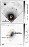 |
Fig. 1. MUSE images of Malin 1, showing the integrated white-light image on the top and the zoom in image of the nuclear region in continuum-subtracted Hα on the bottom. The field of view in the top image is 32″ across while the zoom-in image is 10″ across, with that field marked with the white box in the continuum image. The contours in the top figure reflect the contours of the feature shown in the bottom image, and the orange ellipses in both plots represent the bar identified in Saha et al. (2021), with a radius of 2.6″ (∼4 kpc as calculated by Saha et al. 2021) and centred on the central compact source, which is assumed throughout this paper to be the centre of the galaxy based on the peak luminosity. The central and off-centre compact sources have been labelled in the zoom-in image and both images are orientated with north pointing up and east to the left. |
3. Modelling the core of Malin 1
Figure 1 shows the white-light image of Malin 1 from the MUSE datacube alongside a zoom-in of the central region of the galaxy in Hα, showing that the nuclear region is not a point source, but is instead either an extended source or two compact sources. The orange ellipses in Fig. 1 give the position of the bar component detected by Saha et al. (2021), which has a radius of 2.6″, a Sérsic index of 0.2 and a position angle of 63° as measured anticlockwise from horizontal. These ellipses have been centred on the photometric centre of the galaxy, which coincides with the centre of the brighter of the two clumps. The white contours in the upper plot represent the contours of the structure seen in the Hα image below. One can see that the contours within the nuclear region coincide with those of the bar. Based on these contours we have labelled the two clumps as the central and off-centre compact sources (CCS and OCCS, respectively). In this section, we map out the inner region of Malin 1 to investigate the nature of this structure, with the aim to determine whether it is a nuclear disc, a bar, or globular clusters accreting into the centre of the galaxy.
3.1. Modelling the kinematics at the core of Malin 1
Saha et al. (2021) found that the centre of Malin 1 contained an extended source that they considered to be a bar containing ongoing, asymmetric star formation, leading to a clumpy appearance. Other scenarios that could explain an extended compact source at the centre of a galaxy could be an eccentric stellar disc that formed from the disruption of an infalling GC (Tremaine 1995), where the eccentricity of the disc leads to the appearance of two bright sources. Evidence of a bar or a nuclear disc would be seen in the 2D kinematics in that region: a nuclear disc would present a clear rotation distinct from the underlying disc and an asymmetric velocity dispersion profile within the nuclear disc, while a bar would display a region in which the stellar velocity and h3 are correlated (Bureau & Athanassoula 2005; Iannuzzi & Athanassoula 2015).
As a first step towards modelling the kinematics in this region, the data was spatially binned using the Voronoi tessellation method of Cappellari & Copin (2003). Following Junais et al. (2024) we used a target signal-to-noise ratio (S/N) of 20 and only included spaxels with a minimum S/N of 2 in the range 6050 − 6500 Å. The stellar kinematics were then modelled using the penalised Pixel Fitting (PPXF) code of Cappellari & Emsellem (2004) and Cappellari (2017), using both stellar template spectra of well defined ages and metallicities and emission line spectra to represent the emission features. The stellar template spectra were taken from the MILES stellar library Sánchez-Blázquez et al. (2006), and both the stellar and gas template spectra were convolved with line-of-sight velocity distributions and velocity dispersions to obtain a model spectrum that best fits each binned galaxy spectrum, and low-order additive polynomials were applied to model the flux calibration of the continuum and reduce template mismatch.
The stellar and gas kinematics maps can be seen in Fig. 2 and the stellar h3 and h4 maps are plotted in Fig. 3, with the contours of the nuclear region from Fig. 1 overplotted for reference. No clear distortion is seen in the velocity and velocity dispersion maps within the region of the contours, indicating that the kinematics in this region are dominated by the underlying disc. The h3 and h4 maps, however, appear to show different values in the areas around the two compact sources, which could indicate the presence of a distinct kinematic component. The nature of this component is explored in more detail in Sect. 4.1.
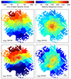 |
Fig. 2. Maps of the stellar (top) and gas (bottom) velocity (left) and velocity dispersion (right) in the central region of Malin 1. The field of view is the same as the bottom plot in Fig. 1, and the contours from that figure are recreated here for reference. A scale bar is given in the bottom right of the gas velocity dispersion plot. |
3.2. Modelling Malin 1 with BUDDI
Another technique to study the central region of Malin 1 is to model the surface-brightness profile to derive the properties of each component present. Furthermore, by modelling and subtracting the brighter components present, fainter and more asymmetric structures may appear in the residual image that would normally be lost in the original data where the other components dominate the light. Thus, this method could be used to study the central region of Malin 1 by subtracting the light from the rest of the galaxy and providing a better view of the nuclear structure.
While this method has been widely applied to photometric data, only in the last decade have IFU data had sufficiently high spatial resolution and wide field of view to apply the same techniques. One code that can apply this modelling to an IFU datacube to extract the clean spectra of each component included in the fit is BUDDI (Bulge–Disc Decomposition of IFU data; Johnston et al. 2017). BUDDI is a wrapper for GALFITM (Häußler et al. 2013), which is a modified form of GALFITM (Peng et al. 2002, 2010) that can model multi-waveband images of a galaxy simultaneously, thus using information from the entire dataset to fit each image by using user-defined Chebyshev polynomials to constrain the variation in the structural parameters over the full wavelength range. As a consequence, GALFITM can derive reasonable estimates of the structural parameters even for images with lower S/N where GALFITM would fail.
BUDDI takes this idea one step further by modelling the galaxy in every image slice within an IFU datacube. Due to the large number of image slices in an IFU datacube, applying GALFITM directly to the datacube is impractical in terms of computing power and time required. BUDDI therefore overcomes this issue by binning the datacube and carrying out the fits in a systematic and reproducible way that can be completed much more rapidly. The final products created by BUDDI are wavelength-dependent models of each morphological component included in the fit, from which the spectra representing the light purely from that component can be extracted either as a one-dimensional (1D) spectrum or in the form of a datacube. These spectra are consequently free from contamination from neighbouring light sources, thus allowing for an independent analysis of each component included in the model.
For this study of Malin 1, BUDDI is the perfect tool to isolate and extract the spectra of the two compact sources at the centre of Malin 1. By modelling the surface-brightness profile of the rest of the galaxy, we can disentangle the spectra of each component included in the model with minimal contamination from the superposition of light from other structures. Thus, with the clean spectra extracted for each compact source in the centre of Malin 1, we can study their properties for the first time. Full details of how BUDDI works can be found in Johnston et al. (2017), and an overview of modelling dwarf galaxies and their NSCs in the Fornax Cluster with BUDDI are described in Johnston et al. (2020). However, for completeness, a brief overview of how BUDDI was used to model the galaxy and extract the spectra of the compact sources is given in Sects. 3.2.1–3.2.5 below.
3.2.1. Step 0: Create a PSF datacube and bad pixel mask
Before running the datacube through BUDDI, a PSF datacube and bad pixel mask must first be created. The PSF datacube models how the PSF varies as a function of wavelength throughout the datacube, thus modelling the smearing of the image due to turbulence in the atmosphere. To create the PSF datacube, two stars were identified within the MUSE datacube’s field of view (FOV). At each wavelength within the datacube, postage stamp images of these two stars were extracted and stacked, and modelled with a Gaussian profile to create a PSF model at each wavelength. Combining these model images thus produced the PSF datacube.
Another important preparation is the bad pixel mask. It can be seen in Fig. 1 that the square MUSE FOV lies at an angle within the image, resulting in many spaxels outside of the MUSE FOV that contain no light and thus show a flux value of 0. Therefore, a badpixel mask was created to mark those spaxels that fall outside of the MUSE FOV and thus eliminate them from the fit.
As can be seen in Fig. 1, the FOV also contains several bright foreground and background objects. Therefore, to minimise their impact on the fit, the regions around these objects were also included in the badpixel mask. A second badpixel mask was created that also masked out the regions of bright emission within the spiral arms. This mask allowed for a better fit to the underlying stellar disc with minimal contamination from the emission regions. Finally, a third bad pixel mask was created that also masked out the emission region around the off-centre compact source but left the central compact source unmasked. For this latter mask, we used a circular aperture centred on the OCCS in the residual datacube from an earlier fit to determine which pixels to mask out. The aim of this mask was to reduce the effect of the off-centre compact source in the fit to the central regions of the galaxy, thus helping to confirm whether the off-centre compact source is a distinct object. The steps outlined in the next sections were carried out using all three of these masks, and in in each of these fits the models for each component within the galaxy were similar, and the emission line analyses showed consistent results for the CCS and the off-centre compact source for each fit. For simplicity, throughout the remainder of this paper, we present only the results using the third bad pixel mask that masks out the emission line regions in the spiral arms and the OCCS from the fit.
3.2.2. Step 1: Obliterate the kinematics
When taking an image slice of a rotating galaxy at a wavelength close to a strong spectral feature, the galaxy may appear asymmetric. One side may be brighter/fainter than the other since it displays light in the stellar continuum while the other side is red or blueshifted into an absorption/emission feature, with further distortion due to the variation in the velocity dispersion as a function of radius within the galaxy. Since GALFITM cannot model non-axisymmetric structures, these effects must be normalised. Consequently, the first step carried out by BUDDI is to measure and obliterate the stellar kinematics across the galaxy, thus ensuring that each image slice within the datacube shows an image of the galaxy at the same rest-frame wavelength.
As in Sect. 3.1, this step is carried out by first binning the datacube using the Voronoi tessellation technique, and then measuring the kinematics of the binned spectra with PPXF. Once the kinematics across the galaxy were measured, the spectra in each spaxel within the datacube were shifted to the closest spectral pixel to correct for the line-of-sight velocity, and broadened to match the maximum velocity dispersion measured within the galaxy. In order to reduce the effects of erroneous measurements due to the background noise, a limit of S/N = 3 per pixel at ∼6000 Å was implemented for the binning step to only include those spaxels that were not dominated by noise.
It should be noted that this correction only applies to the stellar kinematics within the galaxy. When the galaxy also contains gas that corotates with the stars with similar velocities, the kinematics corrections will have the same effect on the gas emission lines, normalising their line-of-sight velocities and broadening their line profiles across the datacube. If the gas corotates with the stars with a difference in the line-of-sight velocity (i.e. > 1 pixel), the kinematics corrections will either under- or over-correct the gas kinematics. The result of this effect is that in the final spectra extracted for each component, the gas emission lines will be broader than in the original datacube, but no flux should be lost since the spectrum is integrated from across the whole galaxy. This latter scenario was found to be true for Malin 1 where the gas was found to corotate with the stars with only a small difference in velocity outside of the central regions of the galaxy. A deeper analysis of the gas kinematics will be carried out in a future work, and an analysis of the gas properties across the galaxy within this datacube is presented in Junais et al. (2024).
3.2.3. Step 2: Model the white-light image
Once the kinematics have been obliterated, the light profile fits can begin. The first step in the fitting process is to create the white-light image of the galaxy, and to fit that image to determine the best-fitting model. This image represents the maximum S/N image of the galaxy, taking advantage of the information over the full spectral range. Thus, this step provides a quick way to determine the best initial estimates for the physical parameters (integrated magnitude, mtot; effective radius, Re; Sérsic index, n; axis ratio, q; and position angle, PA), and number of components for the fits.
In this case, a good model for the host galaxy was achieved using three Sérsic components, with a PSF component representing the central compact source, as shown in Fig. 4. No constraints were used within the fits to force all four components to be centred on the same pixel, and in the final fit the centres of all components were found to be within ∼0.5 pixels (0.1″) of each other. While a discussion on the nature of the three Sérsic components used to model the galaxy is beyond the scope of this paper, the three component fit is consistent with the fits to the disc, bulge and bar components within this galaxy by Barth (2007), Junais et al. (2020) and Saha et al. (2021). We attempted to include a second PSF component to model the off-centre compact source in the nuclear region shown in Fig. 1, but this source was found to be too faint in the continuum to achieve a good model, and the fits failed to converge.
3.2.4. Step 3: Model the narrow-band images
Once a good fit has been achieved to the white-light image, the wavelength information can be introduced. The datacube was rebinned into a series of 10 narrow-band images along the wavelength direction, where these images have higher S/N values than any individual image slice within the datacube. These images were created by stacking equal numbers of image slices along the datacube with wavebands ranging from ∼350 Å in the blue to ∼600 Å in the red due to the logarithmic binning of the datacube in the wavelength direction. The narrow-band images were then modelled, using the results from the previous step as the initial estimates. The fit was run twice, first with a polynomial of an order of 10 to allow for full freedom in the fit parameters, simulating the effect of running GALFIT on each image independently. This step is useful to get an idea of how the structural parameters vary as a function of wavelength, and in this case to understand the effect of emission in these narrow-band images on the fits to the galaxy. However, each narrow-band image was created by combining ∼380 image slices with only a small fraction of these slices showing emission lines, and upon inspection there was found to be little effect in the narrow-band images that cover a strong emission line. Furthermore, the free fits to these images also showed no obvious variations in the fit parameters between the fits to images containing emission and those displaying only stellar continuum.
The second fit then imposes restrictions in the structural parameters by using polynomials of order 2 (i.e. linear variation with wavelength) for the Re, n, PA and q while still allowing mtot to have full freedom. It should be noted that this order is how GALFITM interprets the order of the polynomial, where order 0 means the parameter is not allowed to vary from the initial estimate, order 1 is allowed to vary but must remain constant with wavelength (Chebychev order 0) and order 2 indicates a linear variation with wavelength (Chebychev order 1). Thus, information on the variation in the structural parameters as a function of wavelength was derived. It was found that, in general, the structural parameters for components all three Sérsic components were relatively constant with wavelength, with the scatter being < 10% of the mean value in all parameters, and in many cases, of the order of 2 − 3%.
3.2.5. Step 4: Fit the image slices and extract the spectra
The next stage used the polynomial fits from the previous step to fit the individual image slices in the kinematics-obliterated datacube. The datacube was first split up into batches of ten consecutive image slices to reduce the computing time and avoid memory issues, and these images were then modelled by GALFITM. For these fits, the structural parameters (Re, n, q and PA) were held fixed for each image slice according to the values that were determined by the polynomial fits in the previous step, while mtot was left completely free. It is possible that the structural parameters for the Sérsic components can be quite different in image slices corresponding to the wavelengths of emission features compared to the stellar continuum (see e.g. Johnston et al. 2012). However, in this study we are interested in modelling the underlying stellar continuum only and have masked out the emission line regions in the image slices at those wavelengths. Therefore, the effect on the fit due to any faint emission present in the unmasked regions is considered to be negligible.
Once these fits were completed, the spectrum for each component was created both as a 1D integrated spectrum for that component and as a model datacube. The 1D spectra were derived by plotting the integrated flux from GALFITM for each component as a function of wavelength, and an overview of these 1D spectra are given in Fig. 5. The datacubes were created by stacking the best-fitting model images of each component at each wavelength from GALFITM. A residual datacube was also created by subtracting the model datacubes for each component from the kinematics-obliterated datacube. A zoom in of the core region in this residual datacube can be seen in Fig. 4 in the stellar continuum and in Hα emission. There are a few artefacts in this region in the stellar continuum image, such as a faint spiral arm, but the off-centre compact source becomes clear in the continuum-subtracted Hα emission image. Similarly, there appears to be some over-subtraction of the flux in the Hα emission image, especially around the region of the PSF component representing the CCS. The flux ratio of the pixel with the highest oversubtraction relative to the peak Hα emission in the area of the off-centre compact source is of the order 0.14. This artefact is likely to have several causes. For example, the PSF model used to model the CCS may not have been perfect for the MUSE data at the position of the centre of the galaxy. As described in Sect. 3.2.1, the PSF datacube was created using the variations in the 2D structure of 2 stars within the MUSE FOV. Ideally more stars would have been used, but in this datacube there were no other suitable candidates (i.e. confirmed bright stars based on their 2D light profile and spectra that are far enough from the edge of the FOV and without any bright structures from the galaxy nearby). Additionally, the residual structures of the slicers and channels in the final MUSE datacube makes it hard to create a perfect PSF for the exact position that it will be used in the model. And finally, it is possible that if the CCS is a distinct source, it may not be perfectly modelled as a PSF component, especially in the emission. Since that structure was being modelled across the entire datacube, the PSF component was found to be the best fit (compared to a Sérsic model for example) over the majority of the wavelength range in the stellar continuum. However if it is more extended in the Hα emission, then the excess emission that falls outside of the PSF profile might instead be included in the model for another component, such as Sérsic 2 in this case, leading to an oversubtraction of the Hα emission in that region. Ideally one would want to modify the models used over the wavelength regions of emission lines to account for the different physical distribution of the stars and gas, but currently that step is not within the capabilities of BUDDI.
Consequently, while the continuum for the off-centre compact source couldn’t be modelled with BUDDI, its emission spectrum, with minimal contamination from the light of the rest of the galaxy and the CCS, could still be extracted from this residual datacube using a circular aperture of 4 pixels (0.8″) in radius centred on the source. This aperture was selected since it covered the brightest region of the emission line component without including any light from the regions where the Hα emission may have been oversubtracted. As a test, the analysis carried out in Sect. 4 was repeated with apertures of 3 and 5 pixels (0.6 − 1.0″) in radius, with no significant difference in the results.
Figure 5 displays the extracted spectra for all components. The top plot gives the spectra normalised relative to the integrated flux of the galaxy, where the integrated spectrum from the original datacube (shown in black) was created by masking out the foreground and background objects in order to reduce their contamination in the spectrum. It should be remembered that these spectra represent the total integrated light for each component integrated from their centre out to infinity. Similarly, some emission lines can be seen in these spectra despite our steps to mask out the emission lines in the fits. These lines represent faint emission lines present throughout large regions of the galaxy that are generally too faint to measure in the spectra from individual spaxels or from smaller binned regions, and which again appear stronger in these spectra due to the large areas of the FOV over which the fluxes have been integrated. The bottom plot shows the spectra of each component normalised relative the to mean of their flux differences either side of the region masked out by the notch filter, ∼5870 Å, and offset by an arbitrary amount to allow for a better comparison of their colour gradients and spectra. Since the continuum flux for the spectrum extracted for the off-centre compact source is very faint compared to the emission lines, we instead normalised this spectrum using the mean flux of the CCS component and added an offset to the flux to align it with the other spectra in this figure for easier comparison of the spectrum shape.
4. Analysis
4.1. The structure at the centre of Malin 1
The central region of Malin 1 has a complex morphology, and the aim of this paper is to investigate the different possibilities and determine whether it hosts a nuclear disc, a star-forming bar, or a GC falling into an NSC. The kinematics maps in Figs. 2 and 3 can be used to look for signatures of kinematic components distinct from the main disc, such as a nuclear disc or a bar.
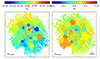 |
Fig. 3. Same as Fig. 2 but showing the stellar h3 (left) and h4 (right) in the central region of Malin 1. |
We first consider the possibility of a nuclear disc. A nuclear disc would appear in the velocity maps as a region with clear rotation that is distinct from the underlying disc. In the velocity plots in Fig. 2, there is no clear indicator of a nuclear disc in the centre of the galaxy, with relatively symmetric velocity curves seen in both the stellar and gas maps. Similarly, both the velocity dispersion maps also appear relatively symmetric. However, the measurements in Fig. 2 mainly show the dominant velocity and velocity dispersion present, while the h3 and h4 polynomials could provide evidence of overlapping components with distinct kinematics. Cole et al. (2014) and Gadotti et al. (2020) describe the signatures for a nuclear disc that formed through dissipative processes (e.g. through bar driven secular evolution) as elevated values of h4 and elevated absolute values of h3. These parameters from the stellar kinematics measurements are plotted in Fig. 3, and appear to show variations in both parameters within the contours marked on the maps. In particular, the h3 and h4 values for the two brightest regions marked by the contours are different, with the upper right region, labelled the OCCS in Fig. 1, displaying more positive h3 and more negative h4 than the lower left region (the CCS), and the lower left region values are more consistent with those or the surrounding disc. This result appears to indicate that the region marked by the contours is unlikely to be a nuclear disc with distinct kinematics relative to the underlying disc, and instead may host two structures with distinct kinematics.
We go on to consider the possibility of a bar. Bureau & Athanassoula (2005) and Iannuzzi & Athanassoula (2015) describe the kinematic signature of a bar as being a region in which the stellar velocity and h3 are correlated due to the superposition of a bar and a disc contributing similar fractions of the light. Such signatures are presented for MUSE observations of barred galaxies in Gadotti et al. (2020), showing that as you move from the centre of the galaxy outwards the stellar velocity and h3 are anticorrelated, then correlated, and then anticorrelated again. The maps in Figs. 2 and 3 are harder to interpret since the potential bar (identified by the contours) and the stellar disc kinematics are not aligned. While there might be a correlation within the contours, such that the upper-right of the contoured region has a higher h3 and higher velocity than the lower-left region, the amplitudes of h3 in these regions are asymmetric, making it difficult to be sure of this correlation. Another possibility is that the OCCS has been captured by the bar and it is orbiting in an x1 orbit going along the bar while corrotating with it. This would naturally explain why both have almost the same alignment, while in the eccentric disk scenario in principle the alignment would be by coincidence. Therefore, from the kinematics it is unclear whether this region is a bar, as proposed by Saha et al. (2021).
If this region does contain a bar, the clumpy appearance could be due to asymmetric star formation. Such a scenario has been seen in the lenticular galaxies IC 676 (Zhou et al. 2020) and PGC 34107 (Lu et al. 2022), and in a number of lenticular and spiral galaxies studied by Díaz-García et al. (2020), where these galaxies were found to host large-scale bars containing asymmetric star formation in young massive clusters. The origin of the gas fuelling the star formation in those clusters could come from two sources-external gas accreted through a merger (Kruijssen et al. 2012), or disc gas losing its angular momentum in the presence of a bar, leading it to migrate in to the inner regions of the galaxy where it can trigger a new episode of star formation (Athanassoula et al. 2013; Consolandi et al. 2017). One can use the angular momentum vectors of the stars and gas to distinguish between these two scenarios, where the accretion of gas scenario would result in the gas kinematics being misaligned relative to the stellar kinematics, while the bar-driven inflow scenario would give more aligned kinematics. One can see in Fig. 2 that the stellar and gas kinematics are relatively well aligned throughout the bar and disc. The global kinematic position angles for the stars and gas velocities were measured using the PAFIT package, which implements the algorithm outlined in Appendix C of Krajnović et al. (2006). The kinematic position angles for the stars and gas were found to be 9 ± 9° and 17 ± 3° as measured anticlockwise from the vertical, respectively. Both these position angles are consistent within their uncertainties, indicating that the gas fuelling the star formation in the point sources at the centre of Malin 1 is most likely to originate from gas migrating in from the extended disc, possibly driven by a bar if present.
While the evidence for a nuclear disc or bar in the inner region of Malin 1 is not very strong, the kinematics maps do appear to show that the region around the OCCS has distinct kinematics relative to the CCS and outside of the contours. Thus is appears likely that the OCCS is a kinematically distinct component, which may be a star cluster falling into the centre of the galaxy or a star forming region within a bar if it is indeed present.
The next step in the analysis was to model the light profile of the galaxy with BUDDI. Images of each component included in the fit are given in Fig. 4 and show that the component labelled Sérsic 2 does appear to have a bar-like structure with a similar size and position angle to the bar modelled by Saha et al. (2021, this work: Re = 1.33″, n = 0.99, PA = 64°. Saha et al. 2021: Re = 1.67″, n = 0.20, PA = 63°).
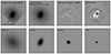 |
Fig. 4. An example of the fit to Malin 1, zoomed in to show a FOV of 20 × 20″. From left to right, the top row shows the white-light images from the original datacube, the best fit model, the residual image from this fit, and the residual image in the region of the Hα wavelength, while the bottom row shows the three Sérsic components that model the host galaxy and the PSF component that models the brighter source at the core, i.e. the CCS. All images are oriented with north up and east to the left, and use the same flux scaling. A scale bar indicating 10″ is given in the top-left plot. |
The fits to the light profile required a PSF component to model the very centre of the galaxy, the region identified as the CCS, but was unable to model the OCCS since it was too faint in the continuum. Instead the spectrum of that component was extracted from the residual datacube. One must always be careful when modelling the light profiles of galaxies to ensure that the components included in the model are real and thus represent a true physical structure within the galaxy. For example, a study of the light profile fits to Elliptical galaxies by Huang et al. (2013) found that while the majority of their sample could be well modelled with three Sérsic components, around 20% of their sample required an additional components. These components modelled either real structures present within the galaxy, such as edge on discs or bars in the case of misclassified S0s, or were used to compensate for irregular structures such as dust lates that affected the light profile. Therefore in the following subsections, we investigate the nature of the CCS and OCCS from their extracted spectra in more detail.
4.2. Confirmation of the location of the CCS and OCCS
If we assume that the CCS and OCCS are distinct sources, one scenario could be that they represent a star cluster falling into an NSC. According to Böker et al. (2002), NSCs are dense but resolved star clusters that are often the brightest and only cluster within a kiloparsec from the photometric centre of the galaxy, and Neumayer et al. (2011) adds to that by showing that NSCs occupy the kinematic core of their host galaxies. The light profile fits in Sect. 3.2.3 found that the centre of the CCS, which was modelled by the PSF component, lies within 0.5 pixels (0.1″) of the centre all the other components included in the fit, indicating that it lies at the photometric centre of the galaxy. However, the fact that it could only be modelled as a PSF profile indicates that the region covered by the CCS is not resolved, making it difficult to determine if it is an NSC or whether it contains light from multiple nuclear components. The PSF FWHM was ∼0.8″, which corresponds to a distance of 1.4 kpc. Within this region, the stellar absorption could originate from a nuclear bulge or disc or a star cluster, while the emission lines could be emitted from a nuclear ring.
In order to better understand the nature of the CCS, the kinematics were measured from the spectrum extracted for the PSF component using PPXF following the same methodology (as described in Sect. 3.2.2), except that a gas component was included in the fit. The stellar and gas kinematics for this component are consistent within 1σ (vLOS, stars = 23 771 ± 16 km s−1, vLOS, gas = 23 802 ± 15 km s−1), indicating that the origin of the stellar absorption and emission lines within the CCS spectrum lie at the same position in the galaxy. The stellar and gas velocities of the binned spectrum from the original datacube in the region of the CCS are vLOS, stars = 23 818 ± 18 km s−1 and vLOS, gas = 23 816 ± 16 km s−1 with velocity dispersions of σstars = 253 ± 12 km s−1 and σgas = 192 ± 10 km s−1, which indicate that the kinematics of the CCS component are consistent with the kinematic core of the galaxy.
The kinematics of the OCCS were measured in the same way, but omitting the stellar absorption spectrum due to the low S/N. This structure was found to have a gas velocity of vLOS, gas = 23 850 ± 16 km s−1, which is consistent with the gas velocity of the CCS to within ∼2.1σ, indicating that these two compact sources are likely to be neighbours.
Since we have the coordinates of the centres of the CCS from the model of the PSF component and the off-centre compact source from the fits with GALFITM, which are given in Table 1, and the parameters for the 2D model fit to the disc of the galaxy (Sérsic 1), we can calculate the deprojected distance between these two objects. The model fit to the extended disc gave a disc major axis with a PA of 48.7° (measured anticlockwise from vertical), an axes ratio, b/a, of 0.82, which results in an inclination of 34.9°. This axes ratio corresponds to an ellipticity of 0.18, which is consistent with that found by Saha et al. (2021). With a separation on sky of 1.05″ or 1.925 kpc and assuming that the sources lay at the main plane of the galaxy, we calculate that the off-centre compact source has a de-projected distance of 2.347 ± 0.013 kpc from the CCS. For comparison, using HI maps of Malin 1 Lelli et al. (2010) measured the PA to be 0 and the inclination, i to be 38 ± 3°, which results in a deprojected distance of 2.45 ± 0.11 kpc between the two objects, which is consistent with our findings.
Details of the coordinates of the centres of each component included in the fit and the off-centre compact source (OCCS), and the flux values for the main emission lines.
As a final step, we can determine whether the off-centre compact source is in a gravitationally bound orbit or not, and thus whether it is likely to be falling into the CCS. Using the PA of the extended stellar disc component (48.7°), and extrapolating inwards the circular velocity vc modeled in Lelli et al. (2010), we find that the projected vc of the OCCS is vc, proj = 130 km s−1. Taking into consideration the geometrical orientation of the HI disk changes this value to 173 km s−1, and mass variations of a factor of two vary this result by only 30%. Either way, given the observed vLOS difference with the CCS of 50 km s−1, the projected vc place the OCCS in a bound orbit, and possibly in a radial orbit along the bar of Malin 1. If we assume the geometry of the HI maps from Lelli et al. (2010) instead (PA = 0 and i = 38), we find that the tangential velocity is vc, proj = 173.72 km s−1. The discrepancy between the geometry derived form the HI and the photometry could be due to some warp or interaction that generated an offset between the stellar and gaseous disks, or it could come from the low spatial resolution HI data. However, it is interesting that both values are less than the velocity dispersion measured at the centre of Malin 1 above and greater than the velocity difference between the two objects, indicating that the off-centre compact source may be on a decaying orbit around the CCS.
4.3. Analysis of the emission line properties
BUDDI models the image of the galaxy at each wavelength, using the constraints on the structural parameters to model the stellar continuum in each image slice. While the areas with strong emission were masked out in the fits, there is likely to be some low level emission throughout the galaxy that can be detected when integrating the light over portions of the field of view, such as the components included in the model fit. Therefore, the emission lines present in the spectra for each component, which can be seen in Fig. 5, represent the faint emission present throughout that component.
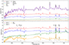 |
Fig. 5. Overview of the spectra extracted for each component shown in Fig. 4 by BUDDI and the off-centre compact source (labelled OCCS). The integrated spectrum from the original datacube is given in black with the spectrum of the best fit given in purple. The spectra for the three Sérsic components, the PSF component representing the CCS and the off-centre compact source are shown in red, blue, green, orange and dark grey, respectively, and the residuals are given in lighter grey. The top plot shows the spectra relative to the flux of the original datacube, while the bottom plot normalises the spectra for the four components to the flux value interpolated from the middle of the notch region and offsets them arbitrarily to better display the differences in gradients and line strengths. Note that in the bottom plot, to better compare the flux of the off-centre compact source it was normalised to the flux of the PSF component in the notch region. The strong feature at 5577 Å is a sky line. |
The BPT diagram of Baldwin et al. (1981) is a powerful tool for comparing various emission line strength ratios and use them to interpret the characteristics of the galaxy. The emission lines were measured using PPXF, modelling both the stellar continuum, absorption features and the gas emission lines simultaneously, using the same method described in Sect. 4.2, except that this time multiplicative Legendre polynomials were used instead of additive polynomials. While using these multiplicative polynomials slows down the fit, they have the advantage of having less of an impact on the line strengths and make the fit more insensitive to dust reddening, thus eliminating the need to include a dust reddening curve. After completing the fit, the emission line strengths for the Hα, Hβ, [OIII]λ5007, [SII]λ6717, [SII]λ6731 and the [NII]λ6583 features were measured and plotted onto the BPT diagram shown in Fig. 6. The line fluxes were not corrected for extinction before plotting them onto the BPT diagram since the line rations are generally considered almost unaffected by extinction due to their proximity in wavelength (see e.g. Belfiore et al. 2015).
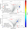 |
Fig. 6. BPT diagrams showing the location of each component modelled by BUDDI as the larger red and yellow points, and of the off-centre compact source as the black filled circle. The open red symbols identify measurements where at least one of the emission lines used had an ANR of less than 3, and so those measurements should be used with caution. Note: the error bars for Sérsic 2 and the off-centre compact source are within the data points. The small coloured points represent the measurements from the original galaxy datacube after binning to increase the S/N, where the colour corresponds to the distance of each binned spectrum from the centre of the galaxy according to the colour bar, and the star symbol is centred on the data point at the centre of the central PSF component. For comparison, the measurements from the MPA-JHU SDSS DR7 galaxies (Brinchmann et al. 2004) have been plotted as grey points, and the central regions of other LSBs from Subramanian et al. (2016) are shown as grey crosses. The black and blue crosses are the emission line ratios from the nuclear region of Malin 1 from Subramanian et al. (2016) and Junais et al. (2020), respectively. The solid curves in both plots represent the maximum starburst line of Kewley et al. (2001), the dashed curve in the bottom plot represents the pure star-forming line of Kauffmann et al. (2003), and the dot-dashed lines in the top and bottom plots differentiate between the Seyfert and LINER classifications according to Kewley et al. (2006) and Cid Fernandes et al. (2010) respectively. |
In order to determine the reliability of the positions on the BPT diagram, the amplitude-to-noise ratio (A/N) for each emission line was measured, where the noise was taken to be the standard deviation of the residual spectrum after subtracting the best fit spectrum from the input spectrum. A limit of A/N = 3 was used, and where at least one emission line in a spectrum had an A/N less than this limit, the measurements were plotted as an open symbol. This situation was found to be true for components labelled as Sérsic 1 and 3, as shown in Fig. 6, while Sérsic 2 and the two compact sources were found to have all emission lines with A/N > 5. The emission line fluxes are listed in Table 1 for each component included in the fit, with those lines with A/N < 3 marked in grey.
For comparison, the process was repeated for the binned spectra extracted from the original datacube (in Sect. 3.2.2) and these measurements are also plotted in Fig. 6, colour coded according to the galactocentric distance of the centre of each bin. Additionally, measurements of other emission-line galaxies from the MPA-JHU SDSS-DR7 catalogue (Brinchmann et al. 2004) have also been plotted as small grey points for reference.
It can be seen that the most extended Sérsic component in Malin 1, Sérsic 1 in Fig. 4, lies within the star-forming region of the BPT diagram, while the other two more compact components, Sérsics 2 and 3, lie within the LINER or composite regions. Similarly, the line ratios for the binned spectra from the original datacube also fall within these LINER or composite regions, with a tentative gradient such that measurements from closer to the centre of the galaxy (darker blue) lie further to the right and as one moves more towards the points further out in the galaxy, especially the few points in the orange and red colours, the points appear to lie closer to the star forming regime. The majority of the points are generally coinsistent with the position of the points for Sérsic 2 in both plots. At this point it should be remembered that Sérsics 1 and 3 have a lower ANR in at least one of their key diagnostic emission lines, as shown in Table 1, and so these line ratios should be used with caution. But in general this result indicates that the ionising gas throughout the galaxy comes from a combination of star formation, active galactic nuclei (AGN), and shocks. These results are consistent with those of Barth (2007), who classed Malin 1 as a LINER galaxy, Subramanian et al. (2016), who identified the galaxy as a LINER galaxy with weak ionisation from both AGN and starbursts, and Junais et al. (2020), who found that Malin 1 lies on the border between LINERS and Seyferts on the BPT diagram. Similarly, these line ratios are consistent with those of the central regions of other LSBs in Subramanian et al. (2016), which are also plotted in Fig. 6.
The point for the CCS lies significantly closer to the AGN/LINER regime in both plots, and interestingly appears to be offset from the measurements from the binned spectra but following the same trend (the star symbol in the plots in Fig. 6 mark the spectrum extracted from CCS at the centre of the galaxy). This effect has been seen before for bulges in Johnston et al. (2017) and for NSCs in dwarf galaxies in Johnston et al. (2020), and simply reflects the strength of BUDDI at cleanly modelling and extracting the light from even faint components within galaxies, whose measurements would otherwise be contaminated by that from the rest of the galaxy. Similarly, the line ratios for the PSF component are offset from those from the nuclear region of Malin 1 from Subramanian et al. (2016) and Junais et al. (2020), shown as the bold crosses in Fig. 6, which is again likely due to the clean extraction of the PSF spectrum in this work. It can be seen that the measurements from the literature are in better agreement with those from the binned spectra from the original datacube, reflecting that the spectra in the literature of the “nucleus” of Malin 1 contain contamination from the light from the rest of the galaxy. Thus, by using this method to cleanly extract the spectrum of the CCS we can assert that this structure is a low-ionisation nuclear emission-line region (LINER), potentially powered by shocks, post-AGB stars and/or low-level accretion activity onto a central massive black hole.
Finally, the OCCS appears to lie on the border with the star-forming regime in both plots. Interestingly, the line strength ratios for this object are similar to those of Sérsic 3 in the top plot of Fig. 6, the most compact Sérsic component in the fit, despite the low ANR of the emission lines in that component. However, the points for these two components do not coincide in the bottom plot, indicating that they do not experience the same mixed ionisation source.
At this point it should be noted that Fig. 4 shows a possible over-subtraction of the Hα emission around the OCCS, which might affect the position in the BPT diagram. As a test of this effect, we extracted two spectra of the surrounding region within annuli of 3 and 5 pixels radius centred on the 4 pixel radius of the OCCS aperture. These spectra were used to “correct” the OCCS spectrum for the possible ovsersubtraction, and the emission lines were measured and analysed in the same way as above. While the position of these corrected spectra in the BPT diagram did move slightly upwards and to the right of the position shown in Fig. 6, the offset was very small and within the error bars. Therefore, the results presented here appear to be minimally affected by this possible oversubtraction of Hα and other emission lines.
Having measured the emission line fluxes for the two compact sources, it is also possible to estimate their SFRs. First, the Hα flux was corrected for dust extinction using the (Calzetti et al. 2000) extinction law with the Balmer decrement,
 (1)
(1)
where F(Hα)o is the observed Hα flux and E(B − V) is the foreground dust reddening along the line of sight:
 (2)
(2)
We assumed an intrinsic Balmer ratio of 2.86 for case-B recombination (Osterbrock 1989) at an electron temperature Te = 10 000 K and density ne = 100 cm−3 (Hummer & Storey 1987). The Hα luminosity of each component, L(Hα) was then calculated using:
 (3)
(3)
where dL is the luminosity distance and, finally, the SFR was determined using the relation:
 (4)
(4)
from Kennicutt et al. (1994). These calculations result in SFRs of 0.012 ± 0.005 M⊙ yr−1 for the CCS and 0.32 ± 0.02 M⊙ yr−1 for the off-centre compact source. The SFRs for both compact sources are of the same order as those of the two star forming regions in the bar of the S0 galaxy IC 676, which have values of 0.08 M⊙ yr−1 and 0.19 M⊙ yr−1 (Zhou et al. 2020). In Malin 1, the SFR of the CCS is significantly lower than the other compact source, in line with what would be expected if the ionisation source is dominated by the LINER as shown in Fig. 6. Furthermore, in the LINER regime one should remember that the Balmer emission lines could also be excited by AGN or shocks rather than only by star formation, and so the SFR derived above from the Hα flux alone may only be considered an upper-limit.
The combination of the similar line-of-sight velocity of the OCCS and the centre of the galaxy with the emission line properties renders it possible that the off-centre compact source consists of one or more unresolved clumps of ongoing star formation that lie very close to the centre of the galaxy, where it is too faint (i.e. low mass) to have a significant stellar continuum at the sampled wavelengths, but bright enough in emission to be detected in specific emission lines.
5. Conclusions
The centre of Malin 1 has long been known to be complex, with evidence of a bar (e.g. Saha et al. 2021) and emission line studies hinting at the presence of both star-formation (e.g. Junais et al. 2020) and LINER (e.g. Barth 2007; Subramanian et al. 2016; Junais et al. 2020) activity. However, the small size of this bar structure (semi-major axis length ∼2.6″ or 4.3 kpc in projection; Saha et al. 2021) has limited attempts to better understand this region. The aim of this paper is to explore the core of Malin 1 with MUSE IFU data to determine the nature of the nuclear region. Analyses of the nuclear kinematics have not revealed any clear evidence of a nuclear disc or a bar with kinematics distinct from the extended disc, but some did suggest that the region around the off-centre compact source contains multiple kinematic components. We applied a careful light profile fit to the entire datacube, finding that the best model consisted of three Sérsic components, a PSF component modelling the CCS, and the spectrum of the OCCS extracted from the residual datacube. Interestingly, one of the Sérsic components in this model is consistent with the bar identified in Saha et al. (2021). This suggests that if the bar is real, it does not show very different kinematics from the rest of the galaxy or it is faint enough that it does not dominate the kinematics in that region. However, the presence of a bar in this region is consistent with the scenario presented by Saha et al. (2021), where the centre of Malin 1 contains a bar hosting asymmetric star formation.
Analyses of the emission line kinematics of the CCS and OCCS reveal that both compact sources lie at the kinematic core of Malin 1, which is consistent with the definition of an NSC by Neumayer et al. (2011). However, the distance to Malin 1 means that it is impossible to resolve this region and confirm that both the stellar continuum and gas emission lines in the region of the CCS have the same origin. If the CCS is in fact an NSC, this result implies that the galaxy contains an NSC onto which a lower-mass, star-forming clump is being accreted. Therefore, we could be witnessing active NSC formation in action. The key emission line ratios were plotted onto BPT diagrams to explore the nature of the ionisation, revealing that the CCS is consistent with a LINER while the OCCS lies in the composite region, very close to the separation between star-forming galaxies and AGN. Additionally, the h3 and h4 maps show higher and lower values, respectively, in the region of the OCCS compared to the CCS and the surrounding disc, suggesting that this region contains an additional structure with distinct kinematics superimposed on the underlying disc. Thus, the large difference in the line strengths of these two targets and the trends in the h3 and h4 maps further adds to the case that they are distinct objects within the core of the galaxy. Assuming that the central compact source is the original and more massive NSC since it lies closer to the kinematic and photometric centre of the galaxy (defined as the peak in the velocity dispersion and light profile, respectively) and has a brighter stellar continuum, the off-centre compact source could either be a star-forming clump containing one or more star clusters that is in the process of falling into the core of the galaxy and which will eventually merge with the central NSC – or a clump of gas infalling into the centre of the galaxy from either outside or from the disc and triggering star formation there. These scenarios are consistent with the wet-migration Guillard et al. (2016) and gas accretion Silk et al. (1987) methods of assembling an NSC. However, with the current resolution available with the available MUSE data, we are unable to distinguish between these two models. Therefore, with future deep photometric observations and additional MUSE pointings to cover the rest of the galaxy, we will be able to further investigate the nature of the core of Malin 1.
Acknowledgments
The authors would like to thank the referee for their useful comments which helped to significantly improve the paper. E.J.J. acknowledges support from FONDECYT Iniciación en investigación 2020 Project 11200263. M.B. acknowledges FONDECYT postdoctorado 2021 No. 3210592 E.J.J., G.G., and T.H.P. gratefully acknowledge support by the ANID BASAL projects ACE210002 and FB210003. J. is grateful for support from the Polish National Science Centre via grant UMO-2018/30/E/ST9/00082. T.H.P. acknowledges support through FONDECYT Regular Project No. 1201016. Y.O.-B. acknowledges support from FONDECYT Postdoctoral 2021, project No. 3210442. P.M.W. gratefully acknowledges support by the German BMBF from the ErUM program (project VLT-BlueMUSE, grant 05A20BAB).
References
- Andersen, D. R., Walcher, C. J., Böker, T., et al. 2008, ApJ, 688, 990 [NASA ADS] [CrossRef] [Google Scholar]
- Ashok, A., Seth, A., Erwin, P., et al. 2023, ApJ, 958, 100 [NASA ADS] [CrossRef] [Google Scholar]
- Athanassoula, E., Machado, R. E. G., & Rodionov, S. A. 2013, MNRAS, 429, 1949 [Google Scholar]
- Bacon, R., Accardo, M., Adjali, L., et al. 2010, SPIE Conf. Ser., 7735, 773508 [Google Scholar]
- Baldwin, J. A., Phillips, M. M., & Terlevich, R. 1981, PASP, 93, 5 [Google Scholar]
- Barth, A. J. 2007, AJ, 133, 1085 [NASA ADS] [CrossRef] [Google Scholar]
- Bekki, K. 2007, PASA, 24, 77 [Google Scholar]
- Bekki, K., Couch, W. J., & Shioya, Y. 2006, ApJ, 642, L133 [Google Scholar]
- Belfiore, F., Maiolino, R., Bundy, K., et al. 2015, MNRAS, 449, 867 [NASA ADS] [CrossRef] [Google Scholar]
- Boissier, S., Boselli, A., Ferrarese, L., et al. 2016, A&A, 593, A126 [NASA ADS] [CrossRef] [EDP Sciences] [Google Scholar]
- Böker, T., Laine, S., van der Marel, R. P., et al. 2002, AJ, 123, 1389 [Google Scholar]
- Bothun, G. D., Impey, C. D., Malin, D. F., & Mould, J. R. 1987, AJ, 94, 23 [NASA ADS] [CrossRef] [Google Scholar]
- Braine, J., Herpin, F., & Radford, S. J. E. 2000, A&A, 358, 494 [NASA ADS] [Google Scholar]
- Brinchmann, J., Charlot, S., White, S. D. M., et al. 2004, MNRAS, 351, 1151 [Google Scholar]
- Bureau, M., & Athanassoula, E. 2005, ApJ, 626, 159 [Google Scholar]
- Calzetti, D., Armus, L., Bohlin, R. C., et al. 2000, ApJ, 533, 682 [NASA ADS] [CrossRef] [Google Scholar]
- Cappellari, M. 2017, MNRAS, 466, 798 [Google Scholar]
- Cappellari, M., & Copin, Y. 2003, MNRAS, 342, 345 [Google Scholar]
- Cappellari, M., & Emsellem, E. 2004, PASP, 116, 138 [Google Scholar]
- Cid Fernandes, R., Stasińska, G., Schlickmann, M. S., et al. 2010, MNRAS, 403, 1036 [Google Scholar]
- Cole, D. R., Debattista, V. P., Erwin, P., Earp, S. W. F., & Roškar, R. 2014, MNRAS, 445, 3352 [NASA ADS] [CrossRef] [Google Scholar]
- Consolandi, G., Dotti, M., Boselli, A., Gavazzi, G., & Gargiulo, F. 2017, A&A, 598, A114 [NASA ADS] [CrossRef] [EDP Sciences] [Google Scholar]
- Das, M., Boone, F., & Viallefond, F. 2010, A&A, 523, A63 [NASA ADS] [CrossRef] [EDP Sciences] [Google Scholar]
- Debattista, V. P., Ferreras, I., Pasquali, A., et al. 2006, ApJ, 651, L97 [NASA ADS] [CrossRef] [Google Scholar]
- den Brok, M., Peletier, R. F., Seth, A., et al. 2014, MNRAS, 445, 2385 [NASA ADS] [CrossRef] [Google Scholar]
- Díaz-García, S., Moyano, F. D., Comerón, S., et al. 2020, A&A, 644, A38 [NASA ADS] [CrossRef] [EDP Sciences] [Google Scholar]
- ESO CPL Development Team 2015, Astrophysics Source Code Library [record ascl:1504.003] [Google Scholar]
- Fahrion, K., Lyubenova, M., van de Ven, G., et al. 2019, A&A, 628, A92 [NASA ADS] [CrossRef] [EDP Sciences] [Google Scholar]
- Fahrion, K., Lyubenova, M., van de Ven, G., et al. 2021, A&A, 650, A137 [NASA ADS] [CrossRef] [EDP Sciences] [Google Scholar]
- Gadotti, D. A., Bittner, A., Falcón-Barroso, J., et al. 2020, A&A, 643, A14 [NASA ADS] [CrossRef] [EDP Sciences] [Google Scholar]
- Galaz, G., Milovic, C., Suc, V., et al. 2015, ApJ, 815, L29 [NASA ADS] [CrossRef] [Google Scholar]
- Galaz, G., Frayer, D. T., Blaña, M., et al. 2022, ApJ, 940, L37 [NASA ADS] [CrossRef] [Google Scholar]
- Georgiev, I. Y., & Böker, T. 2014, MNRAS, 441, 3570 [Google Scholar]
- Gu, Q., Zhao, Y., Shi, L., Peng, Z., & Luo, X. 2006, AJ, 131, 806 [NASA ADS] [CrossRef] [Google Scholar]
- Guillard, N., Emsellem, E., & Renaud, F. 2016, MNRAS, 461, 3620 [Google Scholar]
- Häußler, B., Bamford, S. P., Vika, M., et al. 2013, MNRAS, 430, 330 [Google Scholar]
- Huang, S., Ho, L. C., Peng, C. Y., Li, Z.-Y., & Barth, A. J. 2013, ApJ, 766, 47 [Google Scholar]
- Hummer, D. G., & Storey, P. J. 1987, MNRAS, 224, 801 [NASA ADS] [CrossRef] [Google Scholar]
- Iannuzzi, F., & Athanassoula, E. 2015, MNRAS, 450, 2514 [Google Scholar]
- Johnston, E. J., Aragón-Salamanca, A., Merrifield, M. R., & Bedregal, A. G. 2012, MNRAS, 422, 2590 [Google Scholar]
- Johnston, E. J., Häußler, B., Aragón-Salamanca, A., et al. 2017, MNRAS, 465, 2317 [Google Scholar]
- Johnston, E. J., Puzia, T. H., D’Ago, G., et al. 2020, MNRAS, 495, 2247 [Google Scholar]
- Junais, Boissier, S., Epinat, B., et al. 2020, A&A, 637, A21 [NASA ADS] [CrossRef] [EDP Sciences] [Google Scholar]
- Junais, Weilbacher, P. M., Epinat, B., et al. 2024, A&A, 681, A100 [NASA ADS] [CrossRef] [EDP Sciences] [Google Scholar]
- Kauffmann, G., Heckman, T. M., Tremonti, C., et al. 2003, MNRAS, 346, 1055 [Google Scholar]
- Kennicutt, R. C., Tamblyn, P., & Congdon, C. E. 1994, ApJ, 435, 22 [NASA ADS] [CrossRef] [Google Scholar]
- Kewley, L. J., Dopita, M. A., Sutherland, R. S., Heisler, C. A., & Trevena, J. 2001, ApJ, 556, 121 [Google Scholar]
- Kewley, L. J., Groves, B., Kauffmann, G., & Heckman, T. 2006, MNRAS, 372, 961 [Google Scholar]
- Kormendy, J., & Bender, R. 1999, ApJ, 522, 772 [Google Scholar]
- Krajnović, D., Cappellari, M., de Zeeuw, P. T., & Copin, Y. 2006, MNRAS, 366, 787 [Google Scholar]
- Kruijssen, J. M. D., Pelupessy, F. I., Lamers, H. J. G. L. M., et al. 2012, MNRAS, 421, 1927 [NASA ADS] [CrossRef] [Google Scholar]
- Lauer, T. R., Tremaine, S., Ajhar, E. A., et al. 1996, ApJ, 471, L79 [NASA ADS] [CrossRef] [Google Scholar]
- Lelli, F., Fraternali, F., & Sancisi, R. 2010, A&A, 516, A11 [NASA ADS] [CrossRef] [EDP Sciences] [Google Scholar]
- Lotz, J. M., Telford, R., Ferguson, H. C., et al. 2001, ApJ, 552, 572 [Google Scholar]
- Lu, S., Gu, Q., Ge, X., et al. 2022, ApJ, 927, 215 [NASA ADS] [CrossRef] [Google Scholar]
- Mihos, J. C., & Hernquist, L. 1994, ApJ, 437, L47 [NASA ADS] [CrossRef] [Google Scholar]
- Miller, B. W., & Lotz, J. M. 2007, ApJ, 670, 1074 [NASA ADS] [CrossRef] [Google Scholar]
- Miller, B. W., & Rudie, G. 2008, in Formation and Evolution of Galaxy Bulges, eds. M. Bureau, E. Athanassoula, & B. Barbuy, IAU Symp., 245, 311 [NASA ADS] [Google Scholar]
- Milosavljević, M. 2004, ApJ, 605, L13 [Google Scholar]
- Moore, L., & Parker, Q. A. 2006, PASA, 23, 165 [NASA ADS] [CrossRef] [Google Scholar]
- Neumayer, N., Walcher, C. J., Andersen, D., et al. 2011, MNRAS, 413, 1875 [NASA ADS] [CrossRef] [Google Scholar]
- Neumayer, N., Seth, A., & Böker, T. 2020, A&ARv, 28, 4 [Google Scholar]
- Ordenes-Briceño, Y., Taylor, M. A., Puzia, T. H., et al. 2016, MNRAS, 463, 1284 [CrossRef] [Google Scholar]
- Ordenes-Briceño, Y., Puzia, T. H., Eigenthaler, P., et al. 2018, ApJ, 860, 4 [CrossRef] [Google Scholar]
- Osterbrock, D. E. 1989, Astrophysics of Gaseous Nebulae and Active Galactic Nuclei (Mill Valley: University Science Books) [Google Scholar]
- Peng, C. Y., Ho, L. C., Impey, C. D., & Rix, H.-W. 2002, AJ, 124, 266 [Google Scholar]
- Peng, C. Y., Ho, L. C., Impey, C. D., & Rix, H.-W. 2010, AJ, 139, 2097 [Google Scholar]
- Pickering, T. E., Impey, C. D., van Gorkom, J. H., & Bothun, G. D. 1997, AJ, 114, 1858 [NASA ADS] [CrossRef] [Google Scholar]
- Saha, K., Dhiwar, S., Barway, S., Narayan, C., & Tandon, S. 2021, JApA, 42, 59 [NASA ADS] [Google Scholar]
- Sánchez-Blázquez, P., Peletier, R. F., Jiménez-Vicente, J., et al. 2006, MNRAS, 371, 703 [Google Scholar]
- Silk, J., Wyse, R. F. G., & Shields, G. A. 1987, ApJ, 322, L59 [NASA ADS] [CrossRef] [Google Scholar]
- Soto, K. T., Lilly, S. J., Bacon, R., Richard, J., & Conseil, S. 2016, MNRAS, 458, 3210 [Google Scholar]
- Subramanian, S., Ramya, S., Das, M., et al. 2016, MNRAS, 455, 3148 [NASA ADS] [CrossRef] [Google Scholar]
- Tremaine, S. 1995, AJ, 110, 628 [NASA ADS] [CrossRef] [Google Scholar]
- Tremaine, S. D., Ostriker, J. P., & Spitzer, L. 1975, ApJ, 196, 407 [Google Scholar]
- Turner, M. L., Côté, P., Ferrarese, L., et al. 2012, ApJS, 203, 5 [NASA ADS] [CrossRef] [Google Scholar]
- Weilbacher, P. M., Palsa, R., Streicher, O., et al. 2020, A&A, 641, A28 [NASA ADS] [CrossRef] [EDP Sciences] [Google Scholar]
- Zhou, Z., Ma, J., Zhou, X., & Wu, H. 2020, ApJ, 890, 145 [CrossRef] [Google Scholar]
- Zhu, Q., Xu, D., Gaspari, M., et al. 2018, MNRAS, 480, L18 [CrossRef] [Google Scholar]
All Tables
Details of the coordinates of the centres of each component included in the fit and the off-centre compact source (OCCS), and the flux values for the main emission lines.
All Figures
|
Fig. 1. MUSE images of Malin 1, showing the integrated white-light image on the top and the zoom in image of the nuclear region in continuum-subtracted Hα on the bottom. The field of view in the top image is 32″ across while the zoom-in image is 10″ across, with that field marked with the white box in the continuum image. The contours in the top figure reflect the contours of the feature shown in the bottom image, and the orange ellipses in both plots represent the bar identified in Saha et al. (2021), with a radius of 2.6″ (∼4 kpc as calculated by Saha et al. 2021) and centred on the central compact source, which is assumed throughout this paper to be the centre of the galaxy based on the peak luminosity. The central and off-centre compact sources have been labelled in the zoom-in image and both images are orientated with north pointing up and east to the left. |
| In the text | |
|
Fig. 2. Maps of the stellar (top) and gas (bottom) velocity (left) and velocity dispersion (right) in the central region of Malin 1. The field of view is the same as the bottom plot in Fig. 1, and the contours from that figure are recreated here for reference. A scale bar is given in the bottom right of the gas velocity dispersion plot. |
| In the text | |
|
Fig. 3. Same as Fig. 2 but showing the stellar h3 (left) and h4 (right) in the central region of Malin 1. |
| In the text | |
|
Fig. 4. An example of the fit to Malin 1, zoomed in to show a FOV of 20 × 20″. From left to right, the top row shows the white-light images from the original datacube, the best fit model, the residual image from this fit, and the residual image in the region of the Hα wavelength, while the bottom row shows the three Sérsic components that model the host galaxy and the PSF component that models the brighter source at the core, i.e. the CCS. All images are oriented with north up and east to the left, and use the same flux scaling. A scale bar indicating 10″ is given in the top-left plot. |
| In the text | |
|
Fig. 5. Overview of the spectra extracted for each component shown in Fig. 4 by BUDDI and the off-centre compact source (labelled OCCS). The integrated spectrum from the original datacube is given in black with the spectrum of the best fit given in purple. The spectra for the three Sérsic components, the PSF component representing the CCS and the off-centre compact source are shown in red, blue, green, orange and dark grey, respectively, and the residuals are given in lighter grey. The top plot shows the spectra relative to the flux of the original datacube, while the bottom plot normalises the spectra for the four components to the flux value interpolated from the middle of the notch region and offsets them arbitrarily to better display the differences in gradients and line strengths. Note that in the bottom plot, to better compare the flux of the off-centre compact source it was normalised to the flux of the PSF component in the notch region. The strong feature at 5577 Å is a sky line. |
| In the text | |
|
Fig. 6. BPT diagrams showing the location of each component modelled by BUDDI as the larger red and yellow points, and of the off-centre compact source as the black filled circle. The open red symbols identify measurements where at least one of the emission lines used had an ANR of less than 3, and so those measurements should be used with caution. Note: the error bars for Sérsic 2 and the off-centre compact source are within the data points. The small coloured points represent the measurements from the original galaxy datacube after binning to increase the S/N, where the colour corresponds to the distance of each binned spectrum from the centre of the galaxy according to the colour bar, and the star symbol is centred on the data point at the centre of the central PSF component. For comparison, the measurements from the MPA-JHU SDSS DR7 galaxies (Brinchmann et al. 2004) have been plotted as grey points, and the central regions of other LSBs from Subramanian et al. (2016) are shown as grey crosses. The black and blue crosses are the emission line ratios from the nuclear region of Malin 1 from Subramanian et al. (2016) and Junais et al. (2020), respectively. The solid curves in both plots represent the maximum starburst line of Kewley et al. (2001), the dashed curve in the bottom plot represents the pure star-forming line of Kauffmann et al. (2003), and the dot-dashed lines in the top and bottom plots differentiate between the Seyfert and LINER classifications according to Kewley et al. (2006) and Cid Fernandes et al. (2010) respectively. |
| In the text | |
Current usage metrics show cumulative count of Article Views (full-text article views including HTML views, PDF and ePub downloads, according to the available data) and Abstracts Views on Vision4Press platform.
Data correspond to usage on the plateform after 2015. The current usage metrics is available 48-96 hours after online publication and is updated daily on week days.
Initial download of the metrics may take a while.