| Issue |
A&A
Volume 637, May 2020
|
|
|---|---|---|
| Article Number | A21 | |
| Number of page(s) | 17 | |
| Section | Extragalactic astronomy | |
| DOI | https://doi.org/10.1051/0004-6361/201937330 | |
| Published online | 07 May 2020 | |
First spectroscopic study of ionised gas emission lines in the extreme low surface brightness galaxy Malin 1
1
Aix Marseille Univ, CNRS, CNES, LAM, Marseille, France
e-mail: This email address is being protected from spambots. You need JavaScript enabled to view it.
2
Observatories of the Carnegie Institution for Science, 813 Santa Barbara Street, Pasadena, CA 91101, USA
3
Department of Physics and Astronomy, Stony Brook University, Stony Brook, NY 11794-3800, USA
4
Departamento de Astrofísica, Universidad Complutense de Madrid, 28040 Madrid, Spain
5
European Southern Observatory, Alonso de Cordova 3107, Vitacura, Casilla 19001, Santiago, Chile
6
Centro de Astronomía (CITEVA), Universidad de Antofagasta, Avenida Angamos 601, Antofagasta, Chile
Received:
16
December
2019
Accepted:
20
March
2020
Abstract
Context. Malin 1 is the largest known low surface brightness (LSB) galaxy, the archetype of so-called giant LSB galaxies. The structure and origin of such galaxies are still poorly understood, especially because of the lack of high-resolution kinematics and spectroscopic data.
Aims. We use emission lines from spectroscopic observations of Malin 1 aiming to bring new constraints on the internal dynamics and star formation history of Malin 1.
Methods. We extracted a total of 16 spectra from different regions of Malin 1 and calculated the rotational velocities of these regions from the wavelength shifts and star formation rates from the observed Hα emission line fluxes. We compared our data with existing data and models for Malin 1.
Results. For the first time we present the inner rotation curve of Malin 1, characterised in the radial range r < 10 kpc by a steep rise in the rotational velocity up to at least ∼350 km s−1 (with a large dispersion), which had not been observed previously. We used these data to study a suite of new mass models for Malin 1. We show that in the inner regions dynamics may be dominated by the stars (although none of our models can explain the highest velocities measured) but that at large radii a massive dark matter halo remains necessary. The Hα fluxes derived star formation rates are consistent with an early-type disc for the inner region and with the level found in extended UV galaxies for the outer parts of the giant disc of Malin 1. We also find signs of high metallicity but low dust content for the inner regions.
Key words: galaxies: individual: Malin 1 / galaxies: kinematics and dynamics / galaxies: star formation
© Junais et al. 2020
 Open Access article, published by EDP Sciences, under the terms of the Creative Commons Attribution License (https://creativecommons.org/licenses/by/4.0), which permits unrestricted use, distribution, and reproduction in any medium, provided the original work is properly cited.
1. Introduction
The faint and diffuse galaxies that emit much less light per unit area than normal galaxies are known as low surface brightness (LSB) galaxies. Although there is no clear-cut convention for defining LSB galaxies, they are usually broadly defined as galaxies with a disc central surface brightness (μ0) much fainter than the typical Freeman (1970) value for disc galaxies (μ0, B = 21.65 ± 0.30 mag arcsec−2). Low surface brightness galaxies may account for a very large galaxy population and dark matter (DM) content (Impey & Bothun 1997; Blanton et al. 2005; de Blok & McGaugh 1997). Therefore, understanding this type of galaxies and their rotation curves (RCs), provided we have good kinematics data, could offer some new insights into our current galaxy formation and evolution scenarios.
The LSB galaxies span a wide range of sizes, masses, and morphology from the largest existing galaxies down to the more common dwarfs. Giant low surface brightness galaxies (GLSBs) are a sub-population of LSB galaxies, which have an extremely extended LSB disc with scale lengths ranging from ∼10 kpc to ∼50 kpc (Bothun et al. 1987); GLSBs are also rich in gas content (MHI ∼ 1010 M⊙; Matthews et al. 2001). Despite their low central surface brightness they are sometimes as massive as many “regular” galaxies (see Fig. 3 of Sprayberry et al. 1995). The origin of giant LSBs has been much debated with many propositions, for example face-on collisions (Mapelli & Moore 2008), cooling gas during a merger (Zhu et al. 2018; Saburova et al. 2018), large initial angular momentum (Boissier et al. 2003; Amorisco & Loeb 2016), and accretion from cosmic filaments (Saburova et al. 2019). Few spectroscopic studies were possible in GLSBs (e.g. Saburova et al. 2019), even though this sub-population could offer important information to distinguish between these possibilities.
Malin 1 was discovered in 1986 (Bothun et al. 1987) and is the archetype of GLSB galaxies with a radial extent of ∼120 kpc (Moore & Parker 2006). The galaxy was accidentally discovered in the course of a systematic survey of the Virgo cluster region designed to detect extremely LSB objects (Bothun et al. 1987). Malin 1 has an extrapolated disc central surface brightness of μ0, V ≈ 25.5 mag arcsec−2 (Impey & Bothun 1997). However, despite its faint surface brightness disc, Malin 1 is a massive galaxy with a total absolute magnitude of MV ≈ −22.9 mag (Pickering et al. 1997). It is among the most gas-rich galaxies known with an H I mass of ∼5 × 10¹⁰ M⊙ (Pickering et al. 1997; Matthews et al. 2001). Malin 1 lies in a relatively low-density environment in the large-scale structure, typical for LSB galaxies (Reshetnikov et al. 2010). Using the DisPerSE code (Sousbie 2011) with SDSS/BOSS data, we found Malin 1 lies at a distance of about 10 Mpc from the edge of its closest filament. This relatively low density but proximity to a filament could account for the stability and richness of its extremely huge gaseous disc. The analysis of a Hubble Space Telescope (HST) I-band image by Barth (2007) suggests that Malin 1 has a normal barred inner spiral disc embedded in a huge diffuse LSB envelope, making it similar to galaxies with an extended ultraviolet (XUV) disc found in 30% of nearby galaxies (Thilker et al. 2007). Therefore Malin 1 can also be seen as the most extreme case of this class of galaxies. It is especially interesting to understand the nature of such discs given that more extended galaxies have recently been found (Hagen et al. 2016; Zhang et al. 2018). So far, limited spectroscopic data have been available for Malin 1. A full velocity map is provided by Lelli et al. (2010), but it is obtained from HI data, with a low spatial resolution. In the optical, a spectrum of the central 3 arcsec was obtained by SDSS (region shown in Fig. 1) and is used by Subramanian et al. (2016) to analyze the active galactic nuclei (AGN) properties of a sample of LSBs including Malin 1. Finally, Reshetnikov et al. (2010) obtained spectra along one long-slit passing by the centre of Malin 1 and a companion, but they did not extract from their data an in-plane RC of the galaxy, and rather concentrated on the possible interaction of Malin 1 and its companion. In this work we analyze new spectroscopic data concerning Malin 1. We derive new constraints on the inner kinematics and star formation rate (SFR) surface densities within about 26 kpc. For the sake of comparison, we adopt the same cosmology as Lelli et al. (2010) with H0 = 70 km s−1 Mpc−1, ΩM = 0.27 and ΩΛ = 0.73, which corresponds to a projected angular scale of 1.56 kpc arcsec−1 and a distance of 377 Mpc. This cosmology is consistent with those found in modern cosmological experiments and close to the WMAP9 results (Hinshaw et al. 2013). The basic properties of the galaxy adopted in this work are summarised in Table 1. In Sect. 2 we discuss the data used in this work along with the steps followed for the data reduction. Section 3 gives the major results we obtained in this work. A detailed discussion on the consequences of our results along with a comparison of existing data and models is given in Sect. 4. Section 5 is dedicated to an extensive study of a suite of new Malin 1 mass models. Conclusions are given in Sect. 6.
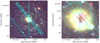 |
Fig. 1. Left: colour composite image of Malin 1 from the CFHT-Megacam NGVS (Ferrarese et al. 2012) u, g, and i band images. The slit positions of our observations are shown as blue rectangles. Right: positions of the 16 apertures in which we could extract a spectrum. The 2016 and 2019 observations are denoted as red and black regions, respectively, along with their designated region names (see Tables 2 and 3). The green circular region indicated in the centre is the location of a SDSS spectrum of Malin 1 with an aperture of 3″ diameter. |
Selected properties of Malin 1.
2. Data and reduction
The spectroscopic data of Malin 1 used in this work were obtained with the IMACS spectrograph at the 6.5 m Magellan Baade telescope in the Las Campanas Observatory, Chile. Two runs of observation took place in 2016 and 2019 with long slits of width 2.5″ and 1.2″, respectively.
In 2016, four slit positions were observed. We extracted a total of 12 spectra from different regions of size 1″ × 2.5″ each, for the three slit positions for which it was possible to obtain a clear signal. This includes a region at ∼26 kpc, which is relatively far from the centre of Malin 1 (see Fig. 1, region f). These observations cover a wavelength range of 4250−7380 Å with a dispersion of 0.378 Å pix−1 and a spectral resolution R ∼ 850. The large width of the slit was chosen to optimise the chance of detecting H II regions within the slit. The orientation of the slits was chosen on the basis of UV images from Boissier et al. (2008). Each of the slit positions had an exposure time of 3 × 1200 s, oriented at a position angle (PA) of 39.95° with respect to the major axis of the galaxy (see Fig. 1). The initial position passes through the galaxy centre. For subsequent positions, the slit positions were shifted from each other by a distance of 2.5″ towards the west (except for the fourth slit position, which was moved about 50″ towards east to pass through distant UV blobs, but we could not detect anything at this position. In order to obtain a precise position for each observations, we simulated the expected continuum flux along the slit, based on an image of Malin 1 acquired during the night of the observations (see Appendix A). A χ2 comparison with our spectral data allowed us to deduce the position of the slit. We estimated the position uncertainty following Avni (1976) and found it to be of the order of 0.1″ (99% confidence level). This process resulted in a small overlap for the slit positions 1 and 2, that is, however, negligible considering the size of the apertures in which we extracted our spectra and thereby each of our apertures are considered as independent regions.
The 2019 observation of Malin 1 was performed using a narrower slit width of 1.2″ oriented at a PA of 0°, along the major axis of the galaxy. The observations were done for a single position with an exposure time of 2 × 1200 s and a wavelength coverage of 3650−6770 Å to obtain a spectral resolution R ∼ 1000. We extracted four spectra from this run for which the [O II] doublet (λ3727,3729) is clearly detected (although the two lines overlap at our resolution), each with an aperture size of 1″ × 1.2″. The average atmospheric seeing measured at the location was ∼1″, with an airmass of 1.4 and a spatial sampling of 0.111″ pix−1 for all the Malin 1 observations.
For both runs, the data reduction and spectral extraction were carried out using standard IRAF1 tasks within the ccdred and onedspec packages. The wavelength calibration was done using a standard HeNeAr arc lamp for each aperture independently. Flux calibration of the extracted spectra from the 2016 observation was done using the reference star LTT 3218 (observed at an airmass of 1.011). We did not perform a flux calibration for the 2019 data, since we do not have a proper reference star for this observation. For illustration purposes, as shown in the fourth row of Fig. 2, we normalised the flux with the Next Generation Virgo cluster Survey (NGVS) u-band photometry in the same aperture as our slit. Since this is not a proper calibration, we do not provide line fluxes in this case. However, we checked that if we adjust the continuum level with this u-band photometry (or with the overlapping spectra from 2016 observations), the [O II]3727/Hα flux ratio obtained is within the values found by Mouhcine et al. (2005).
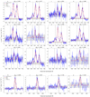 |
Fig. 2. Zoom on the wavelength range of interest for the 16 spectra extracted in this work (12 Hα spectra in the top three rows and 4 [O II] spectra in the fourth row). The solid red curve is the best fit along with its decomposition in single lines shown as thin red dotted lines. The gray dashed line and shaded region indicates the continuum level obtained from the fitting with the 1σ noise level. The black dashed, dotted, and dot-dashed vertical lines indicate the positions of the [N II]6548, Hα and [N II]6583 emission lines, respectively, for the three top rows. The dashed and dotted lines in the bottom row show the position of the two components of the [OII] doublet. The region name and the reduced χ2 are indicated on top of the each panel. |
We were able to extract a total of 16 spectra from different regions of Malin 1 (indicated in Fig. 1), where it was possible to obtain a clear signal for our target emission lines (Hα and [O II]). For each slit position, we started from the peak of emission and moved outwards until no signal was measured around the expected line position (the naming of each region shown in Fig. 1 is based on this). This allowed us to obtain 15 measurements in the central region. We kept any regions for which the peak of the emission line is visible above the noise level (above about 2σ). With this approach, we found we could fit a line (sometimes after spectral re-binning for few regions, as explained further). The inner part of the galaxy, as visible in the broad-band image (Fig. 1), is more extended than the regions for which we could secure a detection. This is because the central region is basically similar to an early-type disc (Barth 2007) with old stars but little gas, thus the emission signal drops quickly to very low level.
After extracting 15 spectra in the inner part of the galaxy, we inspected the rest of the galaxy where we had data and searched for emission, especially those regions close to spiral arms observed in optical wavelength or blobs in the GALEX UV images of Malin 1 (Boissier et al. 2016). For this, we used apertures of the same size as that applied in the inner galaxy, but also larger apertures to increase the signal-to-noise ratio in case of extended emission. However, we were able to recover only one additional spectrum ∼26 kpc away from the centre, close to a compact source visible in the broad-band images from NGVS (Ferrarese et al. 2012), as shown in Fig. 1. This also coincides with a UV blob from the GALEX images of Malin 1. We checked that some of the UV emission overlaps with our aperture, however, the GALEX resolution of about 5″ make this association uncertain. We thus turned to UVIT (Kumar et al. 2012) images of Malin 1, which recently became publicly available and we still found some UV emission at this position (at the UVIT resolution of 1.8″, close to the size of our aperture).
We focussed on the Hα and [O II] emission lines, which were the strongest among those in the observed wavelength range (Hα for the 2016 observation and [O II] for the 2019 observations). For simplicity, we refer to the 2016 and 2019 observations as to the Hα and [O II] observations respectively.
We performed a fit of the emission lines using Python routines implementing a Markov chain Monte Carlo (MCMC) method on a Gaussian line profile to obtain the peak wavelength, flux, and the associated error bars of each emission line (see Appendix A). We fitted the overlapping lines (Hα and [N II]; and the [O II] doublet) simultaneously. Various constraints were applied on the emission lines during the fitting procedure, including a fixed line ratio for the [N II] and [O II] doublets ([N II]6583/[N II]6548 = 2.96 adopted from Ludwig et al. 2012; [O II]3729/[O II]3727 = 0.58 from Pradhan et al. 2006; Comparat et al. 2016). The line ratio of the [O II] doublet depends on the electron density. We performed tests with values covering the range 0.35−1.5 and finally adopted the typical ratio of 0.58, since we do not know for sure the physical conditions in galaxies of very LSB and the choice was not affecting our conclusions. We also fixed the line separations using the laboratory air wavelengths of the emission lines and taking into account the redshift (given in Table 1), where Δλobs = Δλlab(1 + z). The uncertainty in the redshift is negligible (within 1σ error of the wavelength and flux values) and does not affect our results. We also performed a spectral re-binning by a factor 3 for a few of our observations affected by a considerably weaker signal that are at the limit of our detection (regions f, l and p from Fig. 2) to increase the signal-to-noise ratio; this allows us to secure a measurement in these apertures at the price of a lower spectral resolution. The detailed results of our fitting procedure are shown in Fig. 2, Tables 2 and 3.
Extracted data for Malin 1 from the 2016 observation.
Extracted data for Malin 1 from the 2019 observation (2019 data are not flux calibrated).
The robustness of the spectral extraction was checked by the comparison of our central region spectrum (region a) with that of an SDSS spectrum (DR12) of Malin 1 (see Fig. 4). The entire range of both spectra are consistent in terms of the line positions and features. The continuum flux levels in both spectra are also consistent with the expected photometric flux levels measured within their corresponding apertures (shown in Fig. 1) using NGVS g- and i- band images of Malin 1. For this central region, we also performed an underlying stellar continuum fit using the pPXF (penalized pixel-fitting) method by Cappellari (2017), and we also tried to include a broad component to take into account the nucleus activity. However, the stellar continuum subtraction together with the additional active nucleus Hα broad-line component modified our emission line measurement results by less than 1.5σ. Since the continuum is too noisy in many of the apertures, it would not be possible to fit it with pPXF in each apertures. Since the effects in the centre, which should be the largest, do not affect our conclusion, we chose to adopt the same procedure in each aperture (i.e. not fitting the underlying stellar continuum subtraction and broad-line component in the results presented in the paper (Table 2)).
3. Results
3.1. Rotation curve
Rotation curves in LSB galaxies have long been debated (see e.g. de Blok & McGaugh 1997; Pickering et al. 1997; Lelli et al. 2010). The analysis of RCs is of utmost importance in understanding the dynamics and underlying mass distribution and may help to understand the origin of giant LSBs (Saburova et al. 2019). One of the main results of this work is the extraction of a RC for Malin 1 using the observed wavelength of Hα and [O II]3727 emission lines at different positions within the galaxy.
The global systemic velocity (Vsys) of Malin 1 was adopted from Lelli et al. (2010) using H I measurements (see Table 1), which is consistent with the velocity we measure in our Malin 1 centre observation. The observed velocity shift at different regions of the galaxy from Vsys is used for the calculation of the rotational velocities on the galaxy plane as a function of radius. We apply a correction for the galaxy inclination angle and PA (see Table 1), assuming an axi-symmetric geometry and a thin disc. However, a region that is too close to the minor axis of the galaxy (region k) is eliminated from the RC since it has a huge azimuthal correction (cos θ = 0.05 ± 0.02) when re-projecting the observed velocity to the plane of the galaxy (see Table 2). An additional correction for the heliocentric velocity due to the Earth’s motion at the time and location of the observations is also added to the observed velocities (Vhelio = −9.1 km s−1 and −16.3 km s−1 for the 2016 and 2019 data, respectively).
The uncertainties on the velocities are computed by propagating the line-of-sight velocity measurements using the projection parameters of Malin 1 (line of sight and azimuthal deprojections). We quadratically add to this uncertainty that related to the slit positioning described in Sect. 2. The impact of these uncertainties on the de-projected rotation velocities is computed using 10 000 Monte Carlo realisations. The inclination and PA that we adopted are also uncertain. However, we do not take into account these uncertainties, since changing the inclination does not affect the relative position of the points in the RC much. For example, a change of i equal to 3° varies the rotation velocity by ∼15 km s−1. A possible effect of uncertainty in inclination is discussed in Lelli et al. (2010) as well. In addition, in this work we combine the optical RC with the H I RC from Lelli et al. (2010), so it is reasonable to use the same inclination and PA as in that work.
Figure 3 shows the extracted RC of Malin 1. We observe a steep rise in the rotational velocity for the inner regions (inside ∼10 kpc) up to ∼350 km s−1 (with, however, some spread between 200 and 400 km s−1 around a radius of 5 kpc), and a subsequent decline to reach the plateau observed on large scales with H I. Such very high velocities (up to 570 km s−1) are observed in massive spirals (Ogle et al. 2019). Both the Hα and [O II] velocities in our data appear to follow a similar trend and are consistent with each other. A steep inner rise of RC is typical for a high surface brightness (HSB) system. For Malin 1, it is the first time that we observe this behaviour, unlike the slowly rising RC predicted by Pickering et al. (1997) or the poorly resolved inner RC from Lelli et al. (2010) using H I data. The implications of this result and a comparison to existing models and data are discussed in Sect. 4 and motivate the computation of new mass models (Sect. 5).
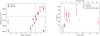 |
Fig. 3. Left: line-of-sight velocity measured from the observed shift in wavelengths for the Hα and [O II] lines (see Tables 2 and 3). The x-axis corresponds to the projected radius on the major axis of the galaxy in the plane of sky. The thick horizontal and vertical dashed lines denote the Vsys and major axis of the galaxy, respectively. Right: rotation curve of Malin 1, projected on the plane of the galaxy. The red and black points indicate the Hα data and [O II] data, respectively. The green open circle shows the Lelli et al. (2010) H I data point in the same radial range. The region name of each point is inidcated with blue letters. |
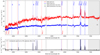 |
Fig. 4. Top: central region spectra of Malin 1. The blue curve is the spectrum extracted in our central 1″ × 2.5″ aperture (region a in Fig. 1). The red curve is the SDSS spectrum of the centre of the galaxy, extracted within its circular optical fibre of diameter 3″ (shown in Fig. 1). The green open circles and black open squares indicate the photometric flux levels obtained within the SDSS and our aperture, respectively, using the NGVS g and i band photometric images of Malin 1. The gray shaded area represent the regions in which we do not have data. Bottom: for comparison, we show the median composite spectrum of all star-forming galaxies (at 0 < z ≲ 1.5) from the SDSS eBOSS observations (Zhu et al. 2015), shifted to the redshift of Malin 1. The blue and red vertical shaded regions indicate the main identified emission and absorption lines. |
3.2. Hα surface brightness and star formation rate
We extract the Hα flux for the 12 regions of Malin 1 discussed in Sect. 2. The observed flux is corrected for inclination and also for the Milky Way foreground Galactic extinction (Schlegel et al. 1998) using the standard Cardelli et al. (1989) dust extinction law. We expect a low dust attenuation within Malin 1 itself, since LSB galaxies in general host very small amounts of dust (Hinz et al. 2007; Rahman et al. 2007). With our data, we can probe the effect of dust attenuation on the Balmer ratio, compared to its theoretical value in the absence of dust. Indeed, we measure both the Hα and Hβ fluxes in eight apertures. The Balmer ratio is however also affected by the underlying stellar absorption. Since our data lack spectral resolution to measure this ratio or signal in the continuum to fit the stellar populations in all of our regions, we applied standard equivalent width (EW) corrections. A large diversity of stellar underlying absorption EW for Hα and Hβ is found in the literature (Moustakas & Kennicutt 2006; Moustakas et al. 2010; Boselli et al. 2013). We first chose to apply the EW corrections that were measured by Gavazzi et al. (2011) for 5000 galaxies (EW Hαabs = 1.3 Å) and by Moustakas et al. (2010) for the representative SINGS sample (EW Hβabs = 2.5 Å). The Balmer ratio of our eight regions was then found within 3σ of the theoretical value of 2.86 for Case B recombination (Osterbrock 1974). The ratio is especially sensitive to the correction to the weaker Hβ line. In order to check the effect of our choice, if we adopt instead another value among the literature, that is EW Hβabs = 5.21 Å (Boselli et al. 2013), the Balmer ratio in the eight regions is now systematically below the theoretical value of 2.86. The Hαabs and Hβabs EW values adopted above from the literature are also consistent with the EW values we obtained from our stellar continuum pPXF fitting of the region a discussed in Sect. 2. Although our EW correction procedure is uncertain, both choices of correction for the underlying stellar absorption lead to a Balmer ratio that is consistent with the absence of dust attenuation. Moreover, Malin 1 is also undetected in the far-infrared with Spitzer and Herschel, which also indicates low attenuation (Boissier et al. 2016). Therefore we can reasonably assume that the Hα flux we measured in this work is only weakly affected from dust attenuation within Malin 1.
Figure 5 shows the extracted Hα surface brightness for the 12 detected regions of Malin 1 plotted as a function of the radius. There is a steep decrease in the surface brightness for the inner regions of Malin 1, similar to a trend that was observed in the Malin 1 I-band surface brightness profile by Barth (2007). This could imply that in the inner regions of Malin 1, the gas profile follows the stellar profile as in normal galaxies (Combes 1999).
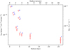 |
Fig. 5. Hα surface brightness measured for different regions of Malin 1. The axis in the right shows the star formation surface density (ΣSFR), corresponding to the observed Hα flux, using the calibration from Boissier (2013). The region name of each point is indicated with blue letters. |
The presence of Hα emission in a galaxy is also a direct indicator of star formation activity at recent times (within ∼10 Myr; e.g. Boissier 2013) provided there is no other source of ionisation like an AGN. However, the effect of a nucleus as a source of ionisation is confined to the single central point of our measurements and cannot have much effect on our kpc scales (see Appendix B on the nuclear activity of Malin 1). Therefore, except for the central region, we can convert with confidence the measured Hα flux to the SFR using standard approximations. We estimate the surface density of SFR (ΣSFR) for the 12 regions of Malin 1 following Boissier (2013) who gives for a Kroupa (2001) initial mass function,
 (1)
(1)
Our apertures cover several kpc. In the central regions of the galaxy with relatively elevated SFR, we expect to find several H II regions per aperture, so that the assumption of quasi-constant star formation history on 10 Myr timescale for Eq. (1) is valid. In the outer aperture, however, star formation is less elevated and may be stochastic so the derived SFR is less robust.
4. Discussions
4.1. Surface density of the SFR
Figure 6 shows a comparison of our Malin 1 estimates of the density of SFR at various radii from Sect. 3.2 compared to the SFR radial profile for samples of disc galaxies from the CALIFA survey that have different morphologies (González Delgado et al. 2016). These profiles are normalised to the half light radius (HLR). We estimate the HLR of Malin 1 to be equal to 2.6″, calculated within 20″ of the centre of the galaxy using the I-band surface brightness profile discussed later and shown in Fig. 7. We adopt this limit such that the comparison is based on the inner galaxy at the centre of Malin 1 as described by Barth (2007) rather than the extended disc because we believe the CALIFA survey (with data from SDSS) corresponds to this inner galaxy better. If we were computing the HLR over the full observed profiles, its value would increase to 18.28″ and the Malin 1 points in Fig. 6 would be much more concentrated.
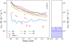 |
Fig. 6. Radial profiles, in units of HLR, of the surface density of the SFR (ΣSFR). The curves correspond to the averages obtained for six morphologies of spiral galaxies from González Delgado et al. (2016). The red points shows our extracted Hα data for Malin 1. The blue dashed line indicates the mean level of ΣSFR in the extended disc of spiral galaxies from Bigiel et al. (2010) with a 1σ level of dispersion (blue shaded region). The error bar in black indicates the typical dispersion among galaxies provided by González Delgado et al. (2016) around each solid curve. |
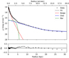 |
Fig. 7. Malin 1 I-band surface brightness decomposition. Bottom panel: difference between the observed surface brightness distribution and the model fit shown in the top panel. |
Our measurements within ∼1.5 HLR behave like an intermediate S0/Sa early-type spiral galaxy (Fig. 6), consistent with the observation from Barth (2007). We also verified that a comparison with the specific SFR radial profile (using the stellar profile in Boissier et al. 2016) leads to the same conclusion. A similar work on two GLSB galaxies Malin 2 and UGC 6614 from Yoachim et al. (in prep.) also shows that GLSB galaxies in general behave like large early-type galaxies at their centre. Our region at 26 kpc from the centre is likely to be part of the extended disc (Barth 2007). Since we detect Hα at only one region really in the extended disc, it is impossible to draw conclusions using this value concerning the overall surface brightness and SFR at that radius. However this surface density of SFR is consistent with the expectations based on the UV blobs luminosity measured in the UV images. It also falls within the 1σ dispersion around the average SFR surface density seen in extended discs of spiral galaxies by Bigiel et al. (2010), as shown in Fig. 6. Finally, a model from Boissier et al. (2016) for Malin 1 also predicts the SFR surface density around this radius to be 0.08 M⊙ Gyr−1 pc−2, which is consistent with our measurement. However it should be kept in mind that the model predicts the azimuthal average SFR, while our measured value value corresponds to a single detected region. Moreover, the detection at 26 kpc is very uncertain owing to the sky level. Deeper observations would help to confirm this and possibly detect other faint H II regions in the extended disc.
4.2. Comparison of our rotation curve with other data
Lelli et al. (2010) provided a RC for Malin 1 using H I data (Fig. 8). However the poor spatial resolution of their data makes it hard to study the dynamics in the inner regions of the galaxy (r < 10 kpc) and especially to measure the mass content of the DM in LSB galaxies.
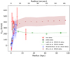 |
Fig. 8. Existing models and data for Malin 1. In addition to the data presented in Fig. 3, the green dotted curve is a model from Lelli et al. (2010), assuming a constant stellar mass-to-light ratio (M⋆/L = 3.4). The brown open circles with the shaded region correspond to an IllustrisTNG100 simulated data from Zhu et al. (2018) for a galaxy similar to Malin 1. The blue open circles indicate the data from Reshetnikov et al. (2010) using stellar absorption lines with the error bars denoted as the blue shaded region. |
Yet another work on spectral analysis of the inner regions of Malin 1 was performed by Reshetnikov et al. (2010) using stellar absorption lines (shown in Fig. 8). However, these authors only provide the radial velocity data corresponding to a single slit position (PA = 55°), which we converted to the rotational velocities in the plane of the galaxy taking into account the same geometrical assumptions we adopt in this work (Sect. 3.1). The rotational velocities from Reshetnikov et al. (2010) within ∼10 kpc are in broad agreement with our data considering their large error bars. This suggests that the gas and stars rotate together in a coherent way in the central regions of Malin 1. Some stellar absorption lines were also detected in very few regions of our data, and these were consistent with our observed RC. However, we prefer not to use these stellar absorption lines considering the poor signal-to-noise ratio and the small number of detected regions. An accurate comparison of the stellar and gaseous dynamics would require, for exmaple IFU data.
In other GLSBs, other behaviours have sometimes been observed, such as counter-rotation in UGC 1922 (Saburova et al. 2018). Yoachim et al. (in prep.) observes a slowly rising RC for the GLSB galaxies Malin 2 and UGC 6614 using stellar absorption lines, unlike the trend we observe for Malin 1 in this work.
4.3. Comparison of our rotation curve with existing models
A mass model for Malin 1 from Lelli et al. (2010) using H I data (shown in Fig. 8), does not capture the highest rotational velocities we observe for the inner regions and do not show the rise of the RC. This could be due to the low resolution of the H I data used as the basis of their modelling. Our new observations with high spatial resolution in the centre of Malin 1 call for a new mass modelling attempt that is consistent with our observed rotational curve, taking into account all the stellar, DM, and gas contributions for the rotational velocity within the galaxy, which is discussed in the Sect. 5.
A recent publication by Zhu et al. (2018) based on the IllustrisTNG simulations also puts forward some interesting results. These authors were able to find a Malin 1 analog with similar features to Malin 1 observations and its vast extended LSB disc in the volume of a 100 Mpc box size simulation. They discuss the formation of a “Malin 1 analog” from the cooling of hot halo gas, triggered by the merger of a pair of intruding galaxies. Their results also include a prediction for the RC of the simulated galaxy with a maximum rotational velocity of 430 km s−1 (shown in Fig. 8), close to the maximal value observed for Malin 1 in our analysis. However, the sudden rise of the inner RC for Malin 1 followed by a decline to ∼200 km s−1 seen in our analysis is not observed in their RC. This comparison demonstrates that our observational results offer a new constraint for this type of simulations in the future or any other model of Malin 1 or Malin 1 analogs. Indeed, LSBs and GLSBs can now be studied in the context of cosmological simulations (Kulier et al. 2019; Martin et al. 2019).
5. New mass modelling
We use our Hα and [O II] RCs in combination with H I measurements from Lelli et al. (2010) and the HST I-band photometry (Barth 2007) to construct a new mass model for Malin 1.
We have the total circular velocity components within a disc galaxy given by
 (2)
(2)
where Vcir is the circular velocity of the galaxy as a function of radius. Vdisc, Vbulge, Vgas, and Vhalo are the stellar disc, stellar bulge, gas, and DM halo velocity components, respectively.
We use the H I gas distribution from Lelli et al. (2010), corrected for the distance adopted, to derive the gas velocity component. However, to constrain the stellar bulge and disc velocity components, we need to make a light profile decomposition of Malin 1, discussed in Sect. 5.1.
5.1. Light profile decomposition
We adopt the I-band light profile provided by Lelli et al. (2010) who combined the HST I-band surface brightness profile of Malin 1 from Barth (2007) for r ≲ 10 kpc (high spatial resolution) and the R-band profile from Moore & Parker (2006) for r ≳ 10 kpc (large spatial extent). This high spatial resolution in the centre is of primordial importance for the RC study, making the use of HST data necessary for the inner part. At larger radii, we check that this profile is consistent with the recent NGVS (Ferrarese et al. 2012) data of Malin 1 (Boissier et al. 2016).
We perform a decomposition of the I-band surface brightness profile following procedures from Barbosa et al. (2015), into a Sérsic bulge, bar and a broken exponential disc component (Erwin et al. 2008) described as
![Mathematical equation: $$ \begin{aligned} I_{\rm d}(r) = S I_0 e^{-\frac{r}{h_{\rm i}}}\left[ 1 + e^{\alpha (r-r_{\mathrm{b} })} \right]^{\frac{1}{\alpha }\left(\frac{1}{h_{\rm i}}-\frac{1}{h_{\rm o}}\right)}. \end{aligned} $$](/articles/aa/full_html/2020/05/aa37330-19/aa37330-19-eq3.gif) (3)
(3)
The broken exponential function consists of a disc with an inner and outer scale length, hi and ho, respectively. The parameters rb is the break radius of the disc and α gives the sharpness of the disc transition. Table 4 and Fig. 7 shows the results of our surface brightness decomposition. These values are in good agreement with the decomposition from Barth (2007), although we obtain a relatively stronger bulge and a weaker bar than in their decomposition. This is a minor difference with negligible effects on our further results. It is well known that bars can cause non-circular motions (Athanassoula & Bureau 1999; Koda & Wada 2002; Chemin et al. 2015). However, the orientation of the bar in Malin 1 (approximately 45° with respect to the PA) could not create major non-circular velocity contributions. As a consequence of the scarcity of measurements, we do not include a bar contribution in our mass modelling. Therefore, to make the mass models, we finally consider two components: the Sérsic bulge obtained as the fit described previously and the “disc”, which is the observed profile minus the bulge (in order to account for all the light, but distinguish the spherical geometry of the bulge). These profiles are further corrected for the inclination to be used in the mass models.
Decomposition parameters obtained for Malin 1 from the fitting results.
5.2. Mass-to-light ratio
During the construction of mass models (Sect. 5.4), the surface brightness values are converted into stellar mass profiles, in some cases by fitting the RC, keeping the stellar mass-to-light ratio as a free parameter. However, it is also possible to fix this ratio on the basis of the colour index profile. Taylor et al. (2011) gives the following empirical relation for the conversion g-i colour to stellar mass-to-light ratio:
 (4)
(4)
where M⋆/Li is the i-band stellar mass-to-light ratio in solar units. The values g and i are the g-band and i-band magnitudes, respectively. We use the above relation to obtain M⋆/Li to a 1σ accuracy of ≈0.1 dex.
We measure a radial profile of the g-i colour from the NGVS images of Malin 1 using the ellipse task in IRAF. Our measured values, computed at the NGVS resolution of ∼1″, are in good agreement with the g-i colour of Malin 1 from Boissier et al. (2016) computed at the GALEX resolution of 5″. Therefore, we use our measured g-i colour profile to obtain a M⋆/Li profile of Malin 1 using the empirical relation given in Eq. (4). Figure 9 shows our extracted colour and M⋆/Li as a function of radius. We carry out a polynomial fit of the order of 3 on the extracted M⋆/Li profile as follows:
 (5)
(5)
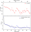 |
Fig. 9. Top: g-i colour profile of Malin 1 measured from the NGVS g-band and i-band images. Bottom: stellar mass-to-light ratio of Malin 1 in i-band measured using the empirical relation from Taylor et al. (2011). The black dashed line indicates the best fit for the measured M⋆/Li. |
This Eq. (5) is only valid for a radius 1″ < r < 40″. For radius r < 1″, we adopt a peak value of M⋆/Li = 3.765 from the colour profile. For r > 40″, we adopt a value of M⋆/Li = 0.379 in order to make a flat profile for the extended disc.
In Sect. 5.4, three assumptions are adopted concerning the M⋆/Li: keeping this ratio as a free parameter, fixing it on the basis of Eq. (5) for the disc, or maintaining the constant M⋆/Li value of 3.765 for the bulge.
5.3. Beam smearing correction
The decomposition of the light profile (Fig. 7) is used to compute the circular velocities of the bulge and disc stellar components. We assume a thin disc and spherical bulge to compute those velocities. These velocities indicate that the rotation is expected to rise more steeply than what is actually observed. One possible reason for this is that the long-slit data is severely affected by resolution owing to the seeing, the size of the slit, and the apertures used to generate the RC in conjunction with the large distance of Malin 1 and the shape of its inner stellar distribution. The impact of this effect can be computed on models, using an observed or modelled light distribution. Epinat et al. (2010) detailed how to perform such computations on velocity fields. In our case, we use the expected geometry of Malin 1 (inclination and position of the major axis) together with the light distribution measured in Hα fit by a third order polynomial supposed to be axisymmetric. High-resolution velocity fields (oversampling by a factor 8 with respect to the actual pixel size) are drawn from idealised RCs derived from stellar mass profiles and we then model the impact of seeing using the recipes presented in Epinat et al. (2010): a convolution of the velocity field weighted by the line flux map normalised by the convolved line flux map. An observational velocity is then derived as the weighted mean of the velocity field on each aperture and the resulting deprojected velocity is computed using the azimuth of the aperture centre and the galaxy inclination. For each stellar component (bulge and disc), the high-resolution mass profiles, obtained both with and without an optimised and varying with radius M/L ratio (see Sect. 5.2), are used to infer the beam smearing curve. The impact of beam smearing is shown in Fig. 10, which clearly illustrates that beam smearing decreases the amplitude of the velocity and offsets the peak of velocity to larger radii. These modifications depend on both the seeing and the slit width. It also clearly shows that depending on the azimuth, the corrections differ and that it is therefore mandatory to compute the beam smearing for each aperture. In the case of the Hα data, the slit is not aligned with the major axis. Apertures that are centred on the major axis therefore have a different value than the ideal case with the slit aligned with the major axis.
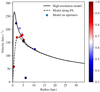 |
Fig. 10. Effect of beam smearing on the RC. The dashed line indicates the high-resolution model, where all the light is supposed to come from the disc, with the M/L that varies as described in Sect. 5.2. The solid line indicates the model after accounting for the effect of the beam smearing: the velocity is computed for apertures of 2.5″, with a slit aligned with the major axis. The dots correspond to the model on the actual apertures of the Hα dataset and their colour indicates their cosine of the azimuth in the galaxy plane. |
The beam smearing and aperture correction are therefore computed for each individual aperture. These curves are then used in the mass model fitting to describe the stellar components. We did not apply such corrections to other components since they are not expected to strongly dominate in the inner regions where the beam smearing is the most severe.
5.4. Dark matter halo
To quantify the distribution of the DM in Malin 1 we use the observation-motivated ISO sphere with a constant central density cored profile (Kent 1986). The core central density profile of the halo is a single power law and the velocity distribution depends on two free parameters: the halo core radius Rc and velocity dispersion σ, providing the asymptotical circular velocity as  , that is,
 (6)
(6)
The mass model is adjusted by changing the parameters.
5.5. Weighting of the rotation curve
The analysis of the mass models depends on the weighting of the RCs, especially when we combine different datasets to construct hybrid RCs as is the case in this study (Hα, [O II] and H I). The use of a chi-square test (χ2) for goodness of fit depends on the variance of the independent variables. The latter variables are the rotation velocities and the variance is the uncertainty associated with the rotation velocity estimation. The method for calculating uncertainties may differ, depending on the nature of the data and on the authors. In addition, the density of uncorrelated Hα rotation velocities is in general larger than for H I RCs and the uncertainties are intrinsically larger. We normalise the uncertainties in attributing the same total weight to the Hα and to the H I datasets to have a similar contribution to the fit from inner and outer regions. Because the weight of uncertainties in a fit is not an absolute but relative quantity, we do not modify the Hα uncertainties but we redistribute the new weights on the H I data only, using the relation given in Korsaga et al. (2019). The weight given to a velocity point is the inverse of its uncertainty. The impact of using different weighing methods is discussed in Sect. 5.6.
5.6. Results of the mass modelling
We present in Fig. 11 the mass model for two cases. On the top panel (model a) the disc and the bulge stellar mass-to-light ratio (M/LBulge) are computed using the colour indices, as discussed in Sect. 5.2, and the disc one (M/LDisc) varies with the radius as shown in Fig. 9. The core radius Rc and the velocity dispersion σ of the DM halo are adjusted using a best-fit model (BFM). In the bottom panel (model b), the four parameters of the model are let free to vary; these are minimised by a BFM and M/LBulge is also forced to be larger than M/LDisc. The parameters of those two models are given in Table 5. Those two models lead to similar halo parameters even though the disc component is about twice as large in model (b) as in model (a) because the larger disc is almost compensated by a weaker bulge in model (b). The DM halo dominates the baryonic components from ∼10 kpc to the end of the RC at ∼100 kpc and the bulge is requested to fit the RC within the first five kpc because the DM halo is not cuspy enough. The main issue of both models is, however, that neither is able to fit the centre of the RC and rotation velocities larger than ∼250 km s−1 correctly.
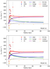 |
Fig. 11. Hybrid RC is plotted using different symbol to represent Hα, [O II] and H I data. The resulting model, plotted using a red line, is the quadratic sum of the gas, disc, bulge, and dark halo components. The lines correspond to the BFM and the bottom and top of the filled area around these lines represent the first and the third percentile around the median (the second percentile) the χ2 distribution ranging from |

Results of the mass models.
We tested the ability of other models to fit these inner points of the RC and report the results for some of those in Table 5. Model (c) is a MDM in which we force the halo to vanish and the disc to be maximal to better fit the inner velocity points of the RC. The χ2 ∼ 8.2 is smaller than for models (a) and (b) meaning that the fit is better on average. This set of parameters is fully compatible with no bulge and no halo but the price to pay for that is an unrealistically large M/LDisc ∼ 20.2 M⊙/L⊙, compared to M/LDisc ∼ 1 ± 0.5 M⊙/L⊙ provided by colour indexes. Because this model has no halo, it only implies two free parameters (the baryonic components). However, if we divide the non-reduced χ2 by the number of data points (19) minus four free-parameters instead of two, we get a reduced χ2 ∼ 9.3 as reported in Table 5, Cols. (3) and (5). Model (d), which is a BFM with four free parameters allowing M/LDisc to be larger than M/LBulge, provides similar results as model (c) with the same absence of bulge, a strong disc, and a weak halo even though it shows that the disc alone cannot adjust the RC. Models (c) and (d) hardly fit some inner velocity points around 300 km s−1, they cannot fit the highest velocity points either; in addition, rotation velocities between 10 kpc and 30 kpc are largely overestimated. We conclude that the “natural” solution when M/LDisc can (non-physically) overpass M/LBulge, is a model without DM halo and without bulge (or very marginal haloes and/or bulges). It is interesting to compare the mass models when the mass-to-light ratio changes or does not change with the radius. Indeed, in the former case, the ratio varies from ∼2 M⊙/L⊙ in the centre of the galaxy, to ∼0.38 M⊙/L⊙ at a radius ∼70 kpc, with a median value of ∼1 within the first 25 kpc, where most of the velocity measurements are and where the disc contribution is the highest (see Fig. 9 and Sect. 5.2).
Best-fit models (d) and (f) use a M/LDisc that does not vary with the radius while this parameter does vary in models (a) and (e). By definition, the best χ2 parameter is obtained when all the parameters are fully free to optimise the fit without any constraints. This is the case for models (d) and (e) for which the physical constraint M/LBulge > M/LDisc is not imposed to the fit; thus we get the smallest χ2 ∼ 7.7, almost 1.7 smaller than for models (a) and (b), which provide χ2 ∼ 13. Comparing models (d) and (e) shows that the average M/LDisc of model (d) is ∼1.5× larger than that of model (e). The consequence is a stronger halo in model (e) to compensate for its weaker M/LDisc at large radius. Model (f) is a variation of model (a) for which the M/LDisc does not change with the radius. The results for models (a) and (f) are very similar. The impact on the halo seen in model (e) with respect to model (d) is no longer observed because the bulge contribution is similar to that of the disc. In order to check if the inner part could be better fitted, we release the constraint on the M/LDisc fixed by colour indexes in model (g), but we keep that on the bulge. As expected, M/LDisc tends to increase almost to the value of M/LBulge, and as a consequence the growing of the disc marginally weakens the DM halo, but does not provide a better fit to the inner velocity rotations; both models (f) and (g) provide almost the same χ2 at ∼13.0 and ∼12.8, respectively.
To take this a step further, because the bulge shape is sharper in the inner region than that of the disc, we maximise M/LBulge to 6 M⊙/L⊙ in model (h) to try to fit the very inner points. This large, but still reasonable M/LBulge value (less than twice as high as that determined using colour indexes) allows the model to pass through the large bulk of dispersed rotation velocities within the 5 inner kpc, but therefore does not allow the model to reach the highest rotation velocities around 400 km s−1. In addition to the fact that this model does not reach velocities above 300 km s−1, it poorly fits the velocities within 0 and 5−10 kpc. We note that M/LDisc and DM parameters are highly degenerated in model (h) since a high M/LDisc and a weak DM halo provide almost the same χ2-value as no disc and a stronger DM halo. However, the principal issue of this model is the slope of the bulge, which is far too sharp to fit the rotation velocities around 200 km s−1 but astonishingly has the right shape to fit a velocity of around 400 km s−1 even though this slope cannot reach these velocities. We clearly see two regimes of velocities at the same radius within the first 5 kpc. The poor fit within the first 5 kpc of model (h) provides a high χ2 ∼ 20 even though it fits the velocities at larger radius, between 10 and 100 kpc, fairly well. In the last four models, from (i) to (l), we study the impact of the stellar distribution geometry on the fits, since this modifies the shape of the model RC. We observe a bright and peaked surface brightness distribution in the centre which could be either a spherical bulge or eventually a bright nucleus. In models (i) and (k) we therefore distribute all the stars in a spherical bulge component, while in models (j) and (l) we set all the stars in a flat disc component. For models (i) and (j) we maximise the stellar components using for both the same fixed mass-to-light ratio, while in models (k) and (l) we test a BFM to let the halo take place. None of those four models allow us to describe the mass distribution of Malin 1 better than any of the others in the sense that BFM models provide almost the same χ2-values but do not help to fit the highest rotation velocities, and if the maximum disc or bulge models permit us to better reach them, they increase the velocity dispersion of residuals velocities, which is also indicated by their high χ2-values.
Models (m) and (n) correspond to the IllustrisTNG100 RC shown in Fig. 8 and discussed in Sect. 4.2. We consider the same BFM as for models (a) and (b), respectively, except that the observed RC is replaced by the IllustrisTNG100 RC, in which we add arbitrary rotation velocities in the first 5 kpc of the galaxy. Indeed, the IllustrisTNG100 RC starts only at a radius of ∼5 kpc while the observed light surface brightness provides constraints within this radius, which are used in the present analysis. We define two different inner slopes for the RC within the first point of the IllustrisTNG100 RC (at a radius of ∼5 kpc). In Table 5, (ls) refers to a “low slope”, which more precisely is an almost solid body shape from 0 to 5 kpc with a velocity gradient of ∼65 km s−1 kpc−1; the label (hs) indicates a “high slope”, which is more precisely a solid body shape RC with two slopes that has a velocity gradient of ∼130 km s−1 kpc−1 from 0 to 2.5 kpc and a lower slope from 2.5 to 5 kpc to smoothly join the IllustrisTNG100 RC. As a consequence of the fact that the IllustrisTNG100 RC amplitude at large radius is twice as large as the observed RC, for both models (m) and (n), the asymptotical velocity dispersion σ is also about twice as large as for previous models, where the actual RC is used. The σ value is almost the same (∼300 km s−1) for models (m) and (n); this value does not depend on the inner slope of the RC or whether the disc and bulge components are used or not. In contrast, in model (b), where all parameters are free, the inner slope has a direct impact on the bulge and disc mass-to-light ratios: a low inner velocity gradient provides a mass model in which no baryonic component is requested, while a high inner velocity gradient allows significant baryonic components. In model (m), for which bulge and disc components are fixed by colours, the core radius tends to match the inner slope of the RC: it is slightly larger/smaller in the case of a low/high inner slope. For model (n), in the case of a high inner RC slope, a high bulge mass-to-light ratio enables us to fit the inner velocities, thus the core radius is more than twice as large as in the case of a low slope where no bulge can fit. The halo mass estimated at the last H I radius (87.2 kpc), using relation (6), gives almost the same value of 3.46 ± 0.05 × 10¹² M⊙ for models (m) and (n) and for the two different inner slopes (ls and hs). This is because the total baryonic mass and baryonic matter distribution do not strongly affect the halo shape. In conclusion, the IllustrisTNG100 RC does not reproduce the different datasets, neither at large nor small radii and no constraint is given on the baryonic components when the RC does not provide any constraint in the inner regions.
In order to compare the various models described in this section and tabulated in Table 5, we plot the parameters of the different mass models in Fig. 12. The isocontours of all the panels involving σ show that this is the best-constrained parameter: all the DM haloes a similar asymptotical velocity around  km s−1. In addition, most of the DM haloes are relatively concentrated with a core radius Rc ∼ 2.5 kpc, this confirms that a massive DM halo is mandatory to adjust the observations. As shown by a different model and the isocontours of panel 5 (Rc versus M/LDisc), the natural trend of the disc is to be massive to extremely massive (for M/LDisc ∼ 6 − 26 M⊙/L⊙), but this is an artefact linked to the lack of velocity resolution in the inner part. The M/LBulge tends to be compatible with that determined by the colour index method if the M/LBulge value is not allowed to overpass M/LBulge value.
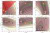 |
Fig. 12. Reduced χ2 contours for models using mass-to-light ratios determined from the photometry projected on the six planes corresponding to the four-dimensional space M/LDisc, M/LBulge, Rc and σ. Each plane is chosen to match the parameters derived for model (b). The forbidden area delimited by the condition M/LBulge ≤ M/LDisc is represented as a red triangle in the top left panel. The contours correspond to the following percentile levels [0, 1, 2, 3, 5, 10, 20, 30, 40, 50, 60, 75, 90] of the distribution; these are labelled by reduced χ2 values. The different symbols, except the large magenta cross, plotted on the six sub-panels, correspond to 10 of the 12 models presented in Table 5 because models (c) and (d) do not fit within the plot limits. Symbols and their colour are described for each model in Table 5. The size of the symbols is random in order to distinguish the different models when they are superimposed. The large white plus symbols used for model (b), do not match with the isocontour centre because of the forbidden volume. The large magenta cross symbols correspond to the median of the 5 percentile of the χ2 distribution. |
As introduced in the Sect. 5.5, the weighting of the rotation velocity coming from H I and optical datasets can differ significantly. In the present study, among the 19 independent velocities measurements, only four come from H I data. In addition, the mean uncertainties are ten times larger in the optical dataset than in the H I dataset (∼53 and ∼5 km s−1 respectively). Because of the importance of the weighting definition, we test the impact of the uncertainties on the model by testing additional methods to weight the data.
We presented the first method in Sect. 5.5. A second method simply consists of using the original error bars, that is those computed independently for the optical and radio datasets. In that case, the output parameters are only marginally modified; this is mainly because each H I error bar is typically ten times smaller than an optical uncertainty, thus providing on average a weight ten times larger than the optical uncertainty, compensating for the fact that only ∼1/5 velocity measurements come from H I data.
In a third method, we give the same weight to all the velocities, independently of their wavelength or their radial and azimuthal locations in the galaxy. This weight is taken as the median of the uncertainties of all the velocities. In that case, the weight of the outer H I data is on average five times smaller than that of the optical data and the mass models tend to be poorly constrained in the outer region, i.e. for radius larger than 30−40 kpc, which is not really acceptable with respect to the large size of Malin 1. Thus rather than going forward with this third method in which the outer H I velocity points have a weak weight, we prefer to discuss the case study for which no H I velocity point is used, but where the H I surface density contribution is kept.
In this fourth configuration for the uncertainties, we only fit the ∼30 inner percents of the RC. When the H I velocities are not used, the disc mass-to-light ratio decreases on average by ∼38% when it is a free parameter (models b, c, d, e, g, h, l; see Table 5), and the bulge mass-to-light ratio decreases from an average value ∼1.2 to 0 M⊙/L⊙ when it is a free parameter (models b, c, d, e, k). Except for case (c), the halo parameters are allowed to freely vary. Using the RCs without the H I components, the halo disappears for cases (i) and (j). To compare the behaviour of the core radius Rc, which becomes infinite when no halo component is involved, cases (c), (i), and (j) are discarded. The mean Rc increases by ∼68% from 3.2 kpc to 5.4 kpc, and the mean velocity dispersion σ grows from ∼129 km s−1 to ∼260 km s−1 (i.e. increases by ∼124%2). Those trends mean that baryonic components are largely when no H I velocities are taken into account while the dark haloes are less concentrated but reach larger velocity dispersions. In terms of mass, using relation (6), when the whole RC is used, the mean halo mass measured at the last H I radius (87.2 kpc) is 5.7 ± 2.3 × 10¹¹ M⊙ while it inconsiderately jumps to 3.3 ± 1.9 × 10¹² M⊙ without H I velocities (i.e. an increase by a factor ∼5.7).
On the other hand, the average halo mass computed without the H I velocity for models (a) and (b) is ∼4.3 × 10¹² M⊙, which is only ∼1.25 times larger that the halo mass estimated using the IllustrisTNG100 RC for the same models (∼3.5 × 10¹² M⊙). This means that if we only had the Hα RC, we would have thought that the IllustrisTNG100 RC gave a compatible model at large radius.
To conclude this discussion, we carried out a final test. Indeed, looking to the observed RC, we note that the Hα rotation velocities strongly decrease between the two largest radii from VMax∼489 km s−1 (at a galacto-centric radius of ∼10.5 kpc) to ∼189 km s−1 (at ∼26.0 kpc), that is to a rotation velocity lower than the average H I velocities of ∼216 km s−1. In order to check that this outermost Hα velocity does not bias the results when we only use the optical data, we rerun the previously labelled “fourth configuration” without considering it. This still increases the disc mass-to-light ratio by ∼31% (instead of ∼38%) and decreases the ratio between the mean halo mass with and without H I from 5.7 to 5.2. Without this outermost Hα velocity, the constraints are still released, however, the disc mass-to-light ratio and the halo parameters do not change much because this outermost Hα data point is weighted by the other 18 optical measurements.
In summary, the new high-resolution and extended RC of Malin 1 does not seem to require a strong DM halo component in the inner part, where the observed stellar mass distribution can explain the dynamics. But a massive DM halo remains necessary to fit the outer regions, whatever the mass model performed. The fit in the inner parts is poor and this may be related to the spatial resolution of the observations, that is at the very limit not to be impacted by beam smearing but also to the assumptions made concerning the geometry of the inner gaseous disc. Ideally, high spectral (R > 2000) and spatial (PSF FWHM < 1″) resolution integral field spectroscopy data could solve these discrepancies by providing at the same time the actual ionised gas line flux spatial distribution and the geometry of the gas in these inner regions, thanks to their 2D kinematics, with much smaller uncertainties. A discussion on the shape of the DM halo (cusp versus core) is therefore out of the scope of this paper.
6. Conclusions
We present a spectroscopic study of the GLSB galaxy Malin 1 using long-slit data from the IMACS spectrograph. In this work we focussed on the Hα and [O II] emission lines detected in 16 different regions of Malin (12 Hα and 4 [O II] detections). The primary results of this work are as follows:
-
We extracted a new RC for Malin 1 using Hα and [O II] emission lines, up to a radial extend of ∼26 kpc.
-
For the first time we observe a steep rise in the inner RC of Malin 1 (within r < 10 kpc), which is not typical for a GLSB or LSB galaxy in general, with points reaching up to at least 350 km s−1 (with a large dispersion) at a few kpc before going back to 200 km s−1, the value found in H I at low resolution.
-
We made an estimate of the Hα surface brightness and SFR surface density of Malin 1 as a function of radius, using the observed Hα emission line flux. The ΣSFR within the inner regions of Malin 1 is consistent with an S0/Sa early type spiral. The region detected at ∼26 kpc from the centre of Malin 1 has a ΣSFR close to the level found in the extended disc of spiral galaxies.
-
An analysis of the observed Balmer line ratio indicates a very low amount of dust attenuation within Malin 1 (consistent with previous works in the infrared).
-
Line ratios, however, point to a relatively high metallicity for the inner regions. The line ratios in the centre are consistent with the previous classification of Malin 1 as a LINER/Seyfert (see Appendix B).
-
The new high-resolution and extended RC of Malin 1 does not seem to require a strong DM halo component in the inner part. In these regions, the observed stellar mass distribution can explain the observed dynamics. However, a massive DM halo is required in the outer regions.
-
The fit of the RC in the inner parts is poor. This may be due to the coarse spatial resolution of the observations, but also to the assumed geometry of the inner gaseous disc (e.g. non-circular velocity contributions due to the bar).
This work allows us to provide new constraints on Malin 1. It will be important in the future, however, to obtain better quality and complementary data for Malin 1, as well as for other giant LSBs, for example with optical IFU such as MUSE or with ALMA, to provide more constraints on the origin of these galaxies. In the recent years, it has become possible to obtain deeper observations with new telescopes such as Dragonfly (Abraham & van Dokkum 2014) or new instrumentation (e.g. MegaCam at CFHT, Hyper Suprime-Cam at Subaru, Dark Energy Survey Camera at the 4 m Blanco telescope). This allows astronomers to revisit the LSB universe, including GLSB galaxies (e.g. Galaz et al. 2015; Boissier et al. 2016; Hagen et al. 2016), extended UV galaxies discovered with GALEX (Gil de Paz et al. 2005; Thilker et al. 2005), and even to define and study the new class of ultra-diffuse galaxies (UDGs) (e.g. van Dokkum et al. 2015; Koda et al. 2015). Galaxies like Malin 1 will be detectable, if they exist, up to redshift 1 with upcoming projects such as SKA (Acero et al. 2017). The recent studies of Malin 1 and other LSBs or UDGs shows that the LSB universe has a “bright” future.
IRAF is distributed by the National Optical Astronomy Observatory, which is operated by the Association of Universities for Research in Astronomy (AURA) under a cooperative agreement with the National Science Foundation.
We do not allow the halo asymptotical velocity  to reach a value higher than the maximum observed rotation velocity VMax = 498 km s−1. We therefore impose an upper limit σMax = 346 km s−1 to the velocity dispersion. Except in cases (c), (i) and (j), where σ = 0 km s−1, σ = σMax, which leads to the average value σ = 260 km s−1.
Acknowledgments
We acknowledge the support by the Programme National Cosmology et Galaxies (PNCG) of CNRS/INSU with INP and IN2P3, co-funded by CEA and CNES. We thank M. Fossati for providing some plotting codes for the line diagnostic diagram and S. Arnouts for his help on the environment of Malin 1. This work also utilised some data from the SDSS DR12 Science Archive Server (SAS) for comparison purposes. Funding for SDSS-III has been provided by the Alfred P. Sloan Foundation, the Participating Institutions, the National Science Foundation, and the US Department of Energy Office of Science. The SDSS-III web site is http://www.sdss3.org/.
References
- Abraham, R. G., & van Dokkum, P. G. 2014, PASP, 126, 55 [NASA ADS] [CrossRef] [Google Scholar]
- Acero, F., Acquaviva, J. T., Adam, R., et al. 2017, ArXiv e-prints [arXiv:1712.06950] [Google Scholar]
- Amorisco, N. C., & Loeb, A. 2016, MNRAS, 459, L51 [NASA ADS] [CrossRef] [Google Scholar]
- Athanassoula, E., & Bureau, M. 1999, ApJ, 522, 699 [NASA ADS] [CrossRef] [Google Scholar]
- Avni, Y. 1976, ApJ, 210, 642 [NASA ADS] [CrossRef] [Google Scholar]
- Baldwin, J. A., Phillips, M. M., & Terlevich, R. 1981, PASP, 93, 5 [NASA ADS] [CrossRef] [EDP Sciences] [Google Scholar]
- Barbosa, C. E., Mendes de Oliveira, C., Amram, P., et al. 2015, MNRAS, 453, 2965 [Google Scholar]
- Barth, A. J. 2007, AJ, 133, 1085 [NASA ADS] [CrossRef] [Google Scholar]
- Bian, F., Kewley, L. J., Dopita, M. A., & Blanc, G. A. 2017, ApJ, 834, 51 [Google Scholar]
- Bigiel, F., Leroy, A., Walter, F., et al. 2010, AJ, 140, 1194 [NASA ADS] [CrossRef] [Google Scholar]
- Blanton, M. R., Lupton, R. H., Schlegel, D. J., et al. 2005, ApJ, 631, 208 [NASA ADS] [CrossRef] [Google Scholar]
- Boissier, S. 2013, in Star Formation in Galaxies, eds. T. D. Oswalt, & W. C. Keel, 6, 141 [Google Scholar]
- Boissier, S., Monnier Ragaigne, D., Prantzos, N., et al. 2003, MNRAS, 343, 653 [NASA ADS] [CrossRef] [Google Scholar]
- Boissier, S., Gil de Paz, A., Boselli, A., et al. 2008, ApJ, 681, 244 [NASA ADS] [CrossRef] [Google Scholar]
- Boissier, S., Boselli, A., Ferrarese, L., et al. 2016, A&A, 593, A126 [NASA ADS] [CrossRef] [EDP Sciences] [Google Scholar]
- Boselli, A., Hughes, T. M., Cortese, L., Gavazzi, G., & Buat, V. 2013, A&A, 550, A114 [NASA ADS] [CrossRef] [EDP Sciences] [Google Scholar]
- Boselli, A., Fossati, M., Consolandi, G., et al. 2018, A&A, 620, A164 [Google Scholar]
- Bothun, G. D., Impey, C. D., Malin, D. F., & Mould, J. R. 1987, AJ, 94, 23 [NASA ADS] [CrossRef] [Google Scholar]
- Braine, J., Herpin, F., & Radford, S. J. E. 2000, A&A, 358, 494 [NASA ADS] [Google Scholar]
- Cappellari, M. 2017, MNRAS, 466, 798 [NASA ADS] [CrossRef] [Google Scholar]
- Cardelli, J. A., Clayton, G. C., & Mathis, J. S. 1989, ApJ, 345, 245 [NASA ADS] [CrossRef] [Google Scholar]
- Chemin, L., Renaud, F., & Soubiran, C. 2015, A&A, 578, A14 [NASA ADS] [CrossRef] [EDP Sciences] [Google Scholar]
- Combes, F. 1999, in H2 in Space, eds. F. Combes, & G. Pineau des Forêts, E.46 [Google Scholar]
- Comparat, J., Zhu, G., Gonzalez-Perez, V., et al. 2016, MNRAS, 461, 1076 [NASA ADS] [CrossRef] [Google Scholar]
- de Blok, W. J. G., & McGaugh, S. S. 1997, MNRAS, 290, 533 [Google Scholar]
- Epinat, B., Amram, P., Balkowski, C., & Marcelin, M. 2010, MNRAS, 401, 2113 [NASA ADS] [CrossRef] [Google Scholar]
- Erwin, P., Pohlen, M., & Beckman, J. E. 2008, AJ, 135, 20 [NASA ADS] [CrossRef] [Google Scholar]
- Ferrarese, L., Côté, P., Cuillandre, J.-C., et al. 2012, ApJS, 200, 4 [NASA ADS] [CrossRef] [Google Scholar]
- Freeman, K. C. 1970, ApJ, 160, 811 [NASA ADS] [CrossRef] [Google Scholar]
- Galaz, G., Milovic, C., Suc, V., et al. 2015, ApJ, 815, L29 [Google Scholar]
- Gavazzi, G., Savorgnan, G., & Fumagalli, M. 2011, A&A, 534, A31 [NASA ADS] [CrossRef] [EDP Sciences] [Google Scholar]
- Gil de Paz, A., Madore, B. F., Boissier, S., et al. 2005, ApJ, 627, L29 [NASA ADS] [CrossRef] [Google Scholar]
- González Delgado, R. M., Cid Fernandes, R., Pérez, E., et al. 2016, A&A, 590, A44 [NASA ADS] [CrossRef] [EDP Sciences] [Google Scholar]
- Hagen, L. M. Z., Seibert, M., Hagen, A., et al. 2016, ApJ, 826, 210 [NASA ADS] [CrossRef] [Google Scholar]
- Hinshaw, G., Larson, D., Komatsu, E., et al. 2013, ApJS, 208, 19 [NASA ADS] [CrossRef] [Google Scholar]
- Hinz, J. L., Rieke, M. J., Rieke, G. H., et al. 2007, ApJ, 663, 895 [NASA ADS] [CrossRef] [Google Scholar]
- Impey, C., & Bothun, G. 1997, ARA&A, 35, 267 [NASA ADS] [CrossRef] [Google Scholar]
- Kent, S. M. 1986, AJ, 91, 1301 [NASA ADS] [CrossRef] [EDP Sciences] [Google Scholar]
- Kewley, L. J., Dopita, M. A., Sutherland, R. S., Heisler, C. A., & Trevena, J. 2001, ApJ, 556, 121 [Google Scholar]
- Kewley, L. J., Groves, B., Kauffmann, G., & Heckman, T. 2006, MNRAS, 372, 961 [NASA ADS] [CrossRef] [Google Scholar]
- Koda, J., & Wada, K. 2002, A&A, 396, 867 [Google Scholar]
- Koda, J., Yagi, M., Yamanoi, H., & Komiyama, Y. 2015, ApJ, 807, L2 [NASA ADS] [CrossRef] [Google Scholar]
- Korsaga, M., Epinat, B., Amram, P., et al. 2019, MNRAS, 490, 2977 [NASA ADS] [CrossRef] [Google Scholar]
- Kroupa, P. 2001, MNRAS, 322, 231 [NASA ADS] [CrossRef] [Google Scholar]
- Kulier, A., Galaz, G., Padilla, N. D., & Trayford, J. W. 2019, MNRAS, submitted [arXiv:1910.05345] [Google Scholar]
- Kumar, A., Ghosh, S. K., Hutchings, J., et al. 2012, in Ultra Violet Imaging Telescope (UVIT) on ASTROSAT, SPIE Conf. Ser., 8443, 84431N [Google Scholar]
- Lelli, F., Fraternali, F., & Sancisi, R. 2010, A&A, 516, A11 [NASA ADS] [CrossRef] [EDP Sciences] [Google Scholar]
- Ludwig, R. R., Greene, J. E., Barth, A. J., & Ho, L. C. 2012, ApJ, 756, 51 [Google Scholar]
- Mapelli, M., & Moore, B. 2008, Astron. Nachr., 329, 948 [NASA ADS] [CrossRef] [Google Scholar]
- Marino, R. A., Rosales-Ortega, F. F., Sánchez, S. F., et al. 2013, A&A, 559, A114 [NASA ADS] [CrossRef] [EDP Sciences] [Google Scholar]
- Martin, G., Kaviraj, S., Laigle, C., et al. 2019, MNRAS, 485, 796 [NASA ADS] [CrossRef] [Google Scholar]
- Matthews, L. D., van Driel, W., & Monnier-Ragaigne, D. 2001, A&A, 365, 1 [NASA ADS] [CrossRef] [EDP Sciences] [Google Scholar]
- Moore, L., & Parker, Q. A. 2006, PASA, 23, 165 [Google Scholar]
- Mouhcine, M., Lewis, I., Jones, B., et al. 2005, MNRAS, 362, 1143 [NASA ADS] [CrossRef] [Google Scholar]
- Moustakas, J., & Kennicutt, R. C., Jr. 2006, ApJS, 164, 81 [NASA ADS] [CrossRef] [Google Scholar]
- Moustakas, J., Kennicutt, R. C., Jr., Tremonti, C. A., et al. 2010, ApJS, 190, 233 [NASA ADS] [CrossRef] [Google Scholar]
- Ogle, P. M., Jarrett, T., Lanz, L., et al. 2019, ApJ, 884, L11 [Google Scholar]
- Osterbrock, D. E. 1974, Astrophysics of Gaseous Nebulae (San Franciso: Freeman) [Google Scholar]
- Pettini, M., & Pagel, B. E. J. 2004, MNRAS, 348, L59 [NASA ADS] [CrossRef] [Google Scholar]
- Pickering, T. E., Impey, C. D., van Gorkom, J. H., & Bothun, G. D. 1997, AJ, 114, 1858 [Google Scholar]
- Pradhan, A. K., Montenegro, M., Nahar, S. N., & Eissner, W. 2006, MNRAS, 366, L6 [NASA ADS] [CrossRef] [Google Scholar]
- Rahman, N., Howell, J. H., Helou, G., Mazzarella, J. M., & Buckalew, B. 2007, ApJ, 663, 908 [Google Scholar]
- Reshetnikov, V. P., Moiseev, A. V., & Sotnikova, N. Y. 2010, MNRAS, 406, L90 [NASA ADS] [CrossRef] [Google Scholar]
- Saburova, A. S., Chilingarian, I. V., Katkov, I. Y., et al. 2018, MNRAS, 481, 3534 [Google Scholar]
- Saburova, A. S., Chilingarian, I. V., Kasparova, A. V., et al. 2019, MNRAS, 489, 4669 [NASA ADS] [CrossRef] [Google Scholar]
- Schawinski, K., Thomas, D., Sarzi, M., et al. 2007, MNRAS, 382, 1415 [NASA ADS] [CrossRef] [Google Scholar]
- Schlegel, D. J., Finkbeiner, D. P., & Davis, M. 1998, ApJ, 500, 525 [NASA ADS] [CrossRef] [Google Scholar]
- Sousbie, T. 2011, MNRAS, 414, 350 [NASA ADS] [CrossRef] [Google Scholar]
- Sprayberry, D., Impey, C. D., Bothun, G. D., & Irwin, M. J. 1995, AJ, 109, 558 [Google Scholar]
- Subramanian, S., Ramya, S., Das, M., et al. 2016, MNRAS, 455, 3148 [NASA ADS] [CrossRef] [Google Scholar]
- Taylor, E. N., Hopkins, A. M., Baldry, I. K., et al. 2011, MNRAS, 418, 1587 [NASA ADS] [CrossRef] [Google Scholar]
- Thilker, D. A., Bianchi, L., Boissier, S., et al. 2005, ApJ, 619, L79 [NASA ADS] [CrossRef] [Google Scholar]
- Thilker, D. A., Bianchi, L., Meurer, G., et al. 2007, ApJS, 173, 538 [NASA ADS] [CrossRef] [Google Scholar]
- van Dokkum, P. G., Romanowsky, A. J., Abraham, R., et al. 2015, ApJ, 804, L26 [NASA ADS] [CrossRef] [Google Scholar]
- Zhang, J., Abraham, R., van Dokkum, P., Merritt, A., & Janssens, S. 2018, ApJ, 855, 78 [Google Scholar]
- Zhu, G. B., Comparat, J., Kneib, J.-P., et al. 2015, ApJ, 815, 48 [NASA ADS] [CrossRef] [Google Scholar]
- Zhu, Q., Xu, D., Gaspari, M., et al. 2018, MNRAS, 480, L18 [NASA ADS] [CrossRef] [Google Scholar]
Appendix A: Estimation of errors
There are mainly two sources of errors in the data provided in this work (see Table 2): the emission line-fitting error and the slit-positioning error. We calculated these errors separately as detailed below. They are combined and propagated to obtain the final errors in each of our quantities of interest.
A.1. Emission line-fitting error
The emission line fitting of the spectra (both Hα and [O II] data) was carried out using an initial formal fitting followed by a MCMC method to obtain the final fitting results. The formal fitting of the spectrum was done using the scipy.optimize.leastsq Python package (see Fig. 2 for fits of continuum + Gaussian emission lines, from which line positions, intensities, line width are derived). From this fit, a model spectra is obtained from the sum of the different component (continuum and lines): Fmodel(λ).
The noise standard deviation σnoise was estimated by subtracting Fmodel from the observed spectrum (Fobs) to obtain the residual spectrum. In order to remove any wavelength dependence, this spectrum was fitted with a polynomial of order 3 that was subtracted to it. We then measured the statistics of this flattened residual spectrum to obtain σnoise.
We then performed an MCMC fitting procedure using an iterative chain of N = 10 000 iterations. In the beginning of each iteration, a synthetic spectrum Fsyn was created using the Fmodel with the addition of a random noise with standard deviation σnoise. At each iteration, we performed again a formal fitting of Fsyn, providing in each case a mock determination of the amplitudes, peak wavelengths, widths, and continuum levels of all the emission line components in the fit. Then histograms of these determinations for each parameters (we focussed on the emission line peak wavelength and flux) were created, inspected, and fitted with a normal distribution. The mean value and standard deviation of each histogram distribution gives our best-fit value and fitting error of a parameter, respectively (see Fig. A.1 for an example).
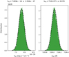 |
Fig. A.1. Example of the MCMC fitting results for the Hα line in the region a (see Table 2). Left and right panels: flux distribution (fHα) and peak wavelength positions (λHα) from the MCMC iterations, respectively. The mean value of this quantities along with their 1σ error bars are labelled on top of each panel. |
A.2. Slit-positioning error
An additional source of error in our measurements comes from the uncertainty in the precise positioning of the slit on the sky during each observation. As discussed in Sect. 2, we had extracted spectra from three different slit positions for the Hα data and a single slit position for the [O II] data. In order to obtain a precise slit position for each observations and the associated uncertainties, we simulated the expected luminosity along the slit on the basis of an image of the galaxy acquired during the 2016 observation, just before the spectroscopic observations (see Fig. A.2). The 2D spectrum at each slit position was collapsed along its spectral axis to obtain the full luminosity distribution passing through the slit (Lslit(pixel)). A mock slit luminosity distribution Lmock(pixel,x, y) is computed from the image for any slit position (x, y), using the same slit width and angle as used in the observations. We started from the position of the slit expected at the telescope during our observations and explored shifts in (x, y) around this position to find the best pixel position for the slit as follows:
![Mathematical equation: $$ \begin{aligned} \chi ^{2}(x,{ y})=\sum _{\rm slit \, pixels} \frac{\Bigg \{L_{\mathrm{slit} }(\mathrm{pixel}) - \left[C \times L_{\mathrm{mock} }(\mathrm{pixel},x,{ y})\right]\Bigg \}^2}{\sigma ^{2}_{\mathrm{pixel} }}, \end{aligned} $$](/articles/aa/full_html/2020/05/aa37330-19/aa37330-19-eq46.gif) (A.1)
(A.1)
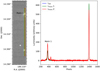 |
Fig. A.2. Left: two mock slits for the slit 1 of our 2016 observations (see Fig. 1), placed on the image of the galaxy acquired during the night of the observation. The two mock slits (green and red) are shifted apart by 1″, with the green slit marking the best slit position obtained in our simulation. Right: luminosity profile along the two mock slits are shown in the left panel (from top to bottom). The blue curve is the luminosity distribution passing through the slit obtained from the 2D spectrum (Lslit(pixel)) of the slit 1 observation (integrated over wavelength to be consistent with the image). |
where  is the total sky level noise and pixel scale Poisson noise measured from Lslit(pixel). The coefficient C is the matching coefficient, computed from the Lslit and Lmock by the following relation:
![Mathematical equation: $$ \begin{aligned} C = \Bigg | \frac{\sum _{\rm slit \, pixels} \left[L_{\mathrm{slit} }(\mathrm{pixel}) \times L_{\mathrm{mock} }(\mathrm{pixel},x,{ y})\right]}{\sum _{\rm slit \, pixels} L^{2}_{\mathrm{mock} }(\mathrm{pixel},x,{ y})} \Bigg |\cdot \end{aligned} $$](/articles/aa/full_html/2020/05/aa37330-19/aa37330-19-eq48.gif) (A.2)
(A.2)
Upon minimizing Eq. (A.1), we obtained a pixel position (x, y) for each of the slit positions with a minimum value of  . The upper and lower confidence levels in the pixel positions were obtained by incrementing the
  value with a Δχ2 value of 6.63 to get a 99% confidence level (see Table 1 of Avni 1976).
For slit positions 1, 2, and 3 of the 2016 observations, the slit-positioning uncertainties were found to be three pixels, one pixel, and one pixel, respectively. For the slit position of the 2019 observation, since we do not have an image on the same night to perfrom the same calculation, we used the maximum uncertainty of three pixels from the 2016 observations to account for this uncertainty. Considering the observational set-up is the same, we think this will cover the positioning error of the telescope and spectrograph.
De-projecting the above-mentioned pixel uncertainties on the sky provides a maximum error of ∼0.3″, and typically of order 0.1″. This uncertainty in the sky coordinates of our regions were propagated while measuring the radius, azimuth angle (cos θ) and Vrot on the galaxy plane (radius and cos θ were computed from the sky coordinates using astropy.coordinates.SkyCoord Python package).
A.3. Combining the error
Since Vrot on the galaxy plane depends on both the observed wavelength λobs and the de-projection angle cos θ, it is affected by both the wavelength fitting error and the error in cos θ due to the slit-positioning uncertainty. We made a quadratic sum of both of theses error contributions to obtain our final error in Vrot shown in this work. In most cases, the error is dominated by the positioning error. Obviously, the wavelength and flux uncertainties are only affected by the fitting error, whereas the radius values are only affected by the slit-positioning error (see Table 2).
Appendix B: Malin 1 nuclear activity and metallicity indication
Barth (2007) classified Malin 1 as a LINER nucleus galaxy with an [N II]6583/Hα flux ratio of 0.85. This is close to our measured flux ratio of [N II]6583/Hα = 0.91 ± 0.06 in the central region of Malin 1. Subramanian et al. (2016) gives a similar classification for Malin 1, placing it in the category of a LINER and composite nuclei with weak ionisation contributions from both AGN and starbursts on the basis of several diagnostics. Our measured central [N II]6583/Hα and [O III]5007/Hβ flux ratios would place Malin 1 on the borderline of LINER-Seyfert classification in a BPT diagram (Baldwin et al. 1981; Kewley et al. 2006) as shown in Fig. B.1. Other LSBs from Subramanian et al. (2016) are located in a similar place as Malin 1 in this diagram. The flux ratios from the other detected regions (six regions in addition to the nucleus) lie in the starburst region but close to the starburst-AGN demarcation line.
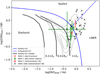 |
Fig. B.1. Line diagnostic BPT diagram with log([N II]6583/Hα) vs. log([O III]5007/Hβ). The red circle and the green triangles indicate the data points of Malin 1 for the nucleus and other detected regions in this work, respectively. The red plus and black crosses are the LSB sample from Subramanian et al. (2016), including Malin 1. The blue solid and dashed lines are defined by Kewley et al. (2001) and Schawinski et al. (2007), respectively, for the separation of AGN from star-forming regions. The gray contours show the distribution of a random sample of nuclear spectra of SDSS galaxies in the redshift range 0.01−1 and stellar mass 109 − 1011 (Boselli et al. 2018). The black solid thick lines show the expected behaviour of star-forming regions as derived from the photo-ionisation models of Kewley et al. (2001) for three different metallicities (0.2, 0.4, 1 Z⊙). |
We also show in Fig. B.1 photo-ionisation models of Kewley et al. (2001), showing that the inner regions of Malin 1 may have a large metallicity. Using the calibration of Pettini & Pagel (2004), the corresponding [N II]6583/Hα ratio indeed points to metallicities about 0.15 dex above solar (or almost solar if we use the improved calibration of Marino et al. 2013). Such metallicities are close to the values expected from the stellar-mass metallicity relationship derived by Bian et al. (2017) for the SDSS galaxies using the same metallicity indicator (and adopting log(M*/M⊙) = 10.87 for Malin 1 after integrating the profile presented in Sect. 5). On the other hand, the high metallicity is at odds with the large amount of gas, but low attenuation (discussed in Sect. 3.2), and absence of detection in CO (Braine et al. 2000).
All Tables
Extracted data for Malin 1 from the 2019 observation (2019 data are not flux calibrated).
All Figures
|
Fig. 1. Left: colour composite image of Malin 1 from the CFHT-Megacam NGVS (Ferrarese et al. 2012) u, g, and i band images. The slit positions of our observations are shown as blue rectangles. Right: positions of the 16 apertures in which we could extract a spectrum. The 2016 and 2019 observations are denoted as red and black regions, respectively, along with their designated region names (see Tables 2 and 3). The green circular region indicated in the centre is the location of a SDSS spectrum of Malin 1 with an aperture of 3″ diameter. |
| In the text | |
|
Fig. 2. Zoom on the wavelength range of interest for the 16 spectra extracted in this work (12 Hα spectra in the top three rows and 4 [O II] spectra in the fourth row). The solid red curve is the best fit along with its decomposition in single lines shown as thin red dotted lines. The gray dashed line and shaded region indicates the continuum level obtained from the fitting with the 1σ noise level. The black dashed, dotted, and dot-dashed vertical lines indicate the positions of the [N II]6548, Hα and [N II]6583 emission lines, respectively, for the three top rows. The dashed and dotted lines in the bottom row show the position of the two components of the [OII] doublet. The region name and the reduced χ2 are indicated on top of the each panel. |
| In the text | |
|
Fig. 3. Left: line-of-sight velocity measured from the observed shift in wavelengths for the Hα and [O II] lines (see Tables 2 and 3). The x-axis corresponds to the projected radius on the major axis of the galaxy in the plane of sky. The thick horizontal and vertical dashed lines denote the Vsys and major axis of the galaxy, respectively. Right: rotation curve of Malin 1, projected on the plane of the galaxy. The red and black points indicate the Hα data and [O II] data, respectively. The green open circle shows the Lelli et al. (2010) H I data point in the same radial range. The region name of each point is inidcated with blue letters. |
| In the text | |
|
Fig. 4. Top: central region spectra of Malin 1. The blue curve is the spectrum extracted in our central 1″ × 2.5″ aperture (region a in Fig. 1). The red curve is the SDSS spectrum of the centre of the galaxy, extracted within its circular optical fibre of diameter 3″ (shown in Fig. 1). The green open circles and black open squares indicate the photometric flux levels obtained within the SDSS and our aperture, respectively, using the NGVS g and i band photometric images of Malin 1. The gray shaded area represent the regions in which we do not have data. Bottom: for comparison, we show the median composite spectrum of all star-forming galaxies (at 0 < z ≲ 1.5) from the SDSS eBOSS observations (Zhu et al. 2015), shifted to the redshift of Malin 1. The blue and red vertical shaded regions indicate the main identified emission and absorption lines. |
| In the text | |
|
Fig. 5. Hα surface brightness measured for different regions of Malin 1. The axis in the right shows the star formation surface density (ΣSFR), corresponding to the observed Hα flux, using the calibration from Boissier (2013). The region name of each point is indicated with blue letters. |
| In the text | |
|
Fig. 6. Radial profiles, in units of HLR, of the surface density of the SFR (ΣSFR). The curves correspond to the averages obtained for six morphologies of spiral galaxies from González Delgado et al. (2016). The red points shows our extracted Hα data for Malin 1. The blue dashed line indicates the mean level of ΣSFR in the extended disc of spiral galaxies from Bigiel et al. (2010) with a 1σ level of dispersion (blue shaded region). The error bar in black indicates the typical dispersion among galaxies provided by González Delgado et al. (2016) around each solid curve. |
| In the text | |
|
Fig. 7. Malin 1 I-band surface brightness decomposition. Bottom panel: difference between the observed surface brightness distribution and the model fit shown in the top panel. |
| In the text | |
|
Fig. 8. Existing models and data for Malin 1. In addition to the data presented in Fig. 3, the green dotted curve is a model from Lelli et al. (2010), assuming a constant stellar mass-to-light ratio (M⋆/L = 3.4). The brown open circles with the shaded region correspond to an IllustrisTNG100 simulated data from Zhu et al. (2018) for a galaxy similar to Malin 1. The blue open circles indicate the data from Reshetnikov et al. (2010) using stellar absorption lines with the error bars denoted as the blue shaded region. |
| In the text | |
|
Fig. 9. Top: g-i colour profile of Malin 1 measured from the NGVS g-band and i-band images. Bottom: stellar mass-to-light ratio of Malin 1 in i-band measured using the empirical relation from Taylor et al. (2011). The black dashed line indicates the best fit for the measured M⋆/Li. |
| In the text | |
|
Fig. 10. Effect of beam smearing on the RC. The dashed line indicates the high-resolution model, where all the light is supposed to come from the disc, with the M/L that varies as described in Sect. 5.2. The solid line indicates the model after accounting for the effect of the beam smearing: the velocity is computed for apertures of 2.5″, with a slit aligned with the major axis. The dots correspond to the model on the actual apertures of the Hα dataset and their colour indicates their cosine of the azimuth in the galaxy plane. |
| In the text | |
|
Fig. 11. Hybrid RC is plotted using different symbol to represent Hα, [O II] and H I data. The resulting model, plotted using a red line, is the quadratic sum of the gas, disc, bulge, and dark halo components. The lines correspond to the BFM and the bottom and top of the filled area around these lines represent the first and the third percentile around the median (the second percentile) the χ2 distribution ranging from |
| In the text | |
|
Fig. 12. Reduced χ2 contours for models using mass-to-light ratios determined from the photometry projected on the six planes corresponding to the four-dimensional space M/LDisc, M/LBulge, Rc and σ. Each plane is chosen to match the parameters derived for model (b). The forbidden area delimited by the condition M/LBulge ≤ M/LDisc is represented as a red triangle in the top left panel. The contours correspond to the following percentile levels [0, 1, 2, 3, 5, 10, 20, 30, 40, 50, 60, 75, 90] of the distribution; these are labelled by reduced χ2 values. The different symbols, except the large magenta cross, plotted on the six sub-panels, correspond to 10 of the 12 models presented in Table 5 because models (c) and (d) do not fit within the plot limits. Symbols and their colour are described for each model in Table 5. The size of the symbols is random in order to distinguish the different models when they are superimposed. The large white plus symbols used for model (b), do not match with the isocontour centre because of the forbidden volume. The large magenta cross symbols correspond to the median of the 5 percentile of the χ2 distribution. |
| In the text | |
|
Fig. A.1. Example of the MCMC fitting results for the Hα line in the region a (see Table 2). Left and right panels: flux distribution (fHα) and peak wavelength positions (λHα) from the MCMC iterations, respectively. The mean value of this quantities along with their 1σ error bars are labelled on top of each panel. |
| In the text | |
|
Fig. A.2. Left: two mock slits for the slit 1 of our 2016 observations (see Fig. 1), placed on the image of the galaxy acquired during the night of the observation. The two mock slits (green and red) are shifted apart by 1″, with the green slit marking the best slit position obtained in our simulation. Right: luminosity profile along the two mock slits are shown in the left panel (from top to bottom). The blue curve is the luminosity distribution passing through the slit obtained from the 2D spectrum (Lslit(pixel)) of the slit 1 observation (integrated over wavelength to be consistent with the image). |
| In the text | |
|
Fig. B.1. Line diagnostic BPT diagram with log([N II]6583/Hα) vs. log([O III]5007/Hβ). The red circle and the green triangles indicate the data points of Malin 1 for the nucleus and other detected regions in this work, respectively. The red plus and black crosses are the LSB sample from Subramanian et al. (2016), including Malin 1. The blue solid and dashed lines are defined by Kewley et al. (2001) and Schawinski et al. (2007), respectively, for the separation of AGN from star-forming regions. The gray contours show the distribution of a random sample of nuclear spectra of SDSS galaxies in the redshift range 0.01−1 and stellar mass 109 − 1011 (Boselli et al. 2018). The black solid thick lines show the expected behaviour of star-forming regions as derived from the photo-ionisation models of Kewley et al. (2001) for three different metallicities (0.2, 0.4, 1 Z⊙). |
| In the text | |
Current usage metrics show cumulative count of Article Views (full-text article views including HTML views, PDF and ePub downloads, according to the available data) and Abstracts Views on Vision4Press platform.
Data correspond to usage on the plateform after 2015. The current usage metrics is available 48-96 hours after online publication and is updated daily on week days.
Initial download of the metrics may take a while.