| Issue |
A&A
Volume 686, June 2024
|
|
|---|---|---|
| Article Number | A266 | |
| Number of page(s) | 18 | |
| Section | Stellar structure and evolution | |
| DOI | https://doi.org/10.1051/0004-6361/202348093 | |
| Published online | 21 June 2024 | |
Extremely metal-poor stars in the Fornax and Carina dwarf spheroidal galaxies⋆
1
Dipartimento di Fisica e Astronomia, Universitá degli Studi di Firenze, Via G. Sansone 1, 50019 Sesto Fiorentino, Italy
e-mail: This email address is being protected from spambots. You need JavaScript enabled to view it.
2
Physics Institute, Laboratoire d’astrophysique, École Polytechnique Fédérale de Lausanne (EPFL), Observatoire, 1290 Versoix, Switzerland
3
European Southern Observatory, Karl-Schwarzschild-str. 2, 85748 Garching bei München, Germany
4
GEPI, Observatoire de Paris, Université PSL, CNRS, 5 Place Jules Janssen, 92190 Meudon, France
5
INAF/Osservatorio Astrofisico di Arcetri, Largo E. Fermi 5, 50125 Firenze, Italy
6
Dipartimento di Fisica e Astronomia, Università degli Studi di Bologna, Via Gobetti 93/2, 40129 Bologna, Italy
7
Institute of Astronomy of the Russian Academy of Sciences, Pyatnitskaya st. 48, 119017 Moscow, Russia
8
Department of Physics and Astronomy, University of Victoria, PO Box 3055 STN CSC, Victoria BC V8W 3P6, Canada
9
Université Côte d’Azur, Observatoire de la Côte d’Azur, CNRS, Laboratoire Lagrange, Nice, France
10
Departamento de Ciencias Físicas, Facultad de Ciencias Exactas, Universidad Andrés Bello, Fernández Concha 700, Las Condes, Santiago, Chile
11
Vatican Observatory, V00120 Vatican City State, Italy
12
Departamento de Fisica, Universidade Federal de Santa Catarina, Trinidade, 88040-900 Florianopolis, Brazil
Received:
27
September
2023
Accepted:
5
January
2024
Abstract
We present our analysis of VLT/UVES and X-shooter observations of six very metal-poor stars, including four stars at [Fe/H] ≈ −3 in the Fornax and Carina dwarf spheroidal (dSph) galaxies. To date, this metallicity range in these two galaxies has not yet been investigated fully, or at all in some cases. The chemical abundances of 25 elements are presented, based on 1D and local thermodynamic equilibrium (LTE) model atmospheres. We discuss the different elemental groups, and find that α- and iron-peak elements in these two systems are generally in good agreement with the Milky Way halo at the same metallicity. Our analysis reveals that none of the six stars we studied exhibits carbon enhancement, which is noteworthy given the prevalence of carbon-enhanced metal-poor stars without s-process enhancement (CEMP-no) in the Galaxy at similarly low metallicities. Our compilation of literature data shows that the fraction of CEMP-no stars in dSph galaxies is significantly lower than in the Milky Way, and than in ultra-faint dwarf galaxies. Furthermore, we report the discovery of the lowest metallicity, [Fe/H] = −2.92, r-process rich (r-I) star in a dSph galaxy. This star, fnx_06_019, has [Eu/Fe] = +0.8, and also shows enhancement of La, Nd, and Dy, [X/Fe] > +0.5. Our new data in Carina and Fornax help populate the extremely low metallicity range in dSph galaxies, and add to the evidence of a low fraction of CEMP-no stars in these systems.
Key words: stars: abundances / galaxies: dwarf / galaxies: evolution / Local Group
Based on UVES and X-shooter observations collected at the ESO, program ID 0100.D–0820 and 094.D–0853.
© The Authors 2024
 Open Access article, published by EDP Sciences, under the terms of the Creative Commons Attribution License (https://creativecommons.org/licenses/by/4.0), which permits unrestricted use, distribution, and reproduction in any medium, provided the original work is properly cited.
This article is published in open access under the Subscribe to Open model. This email address is being protected from spambots. You need JavaScript enabled to view it. to support open access publication.
1. Introduction
Our aim is to understand the characteristics of the first stars formed in the universe from their imprints on low-mass stars in dwarf spheroidal (dSph) galaxies. The stellar abundance trends and dispersion of the most metal-poor stars reveal the nature of the now disappeared first stellar generation (e.g., mass, numbers), and the level of homogeneity of the primitive interstellar medium (ISM; e.g., size and/or mass of star-forming regions), as well as the nature and energy of the first supernovae (e.g., Koutsouridou et al. 2023). The proximity of the Local Group dSph galaxies allows the chemical abundances to be derived in individual stars at comparable quality to the Milky Way (MW). The confrontation of galaxies with very different evolutionary paths brings crucial information on the universality of the star formation processes and chemical enrichment.
Carina, Sextans, Sculptor, and Fornax are four Local Group dSph galaxies that have triggered strong observational efforts from the galactic archaeology community. They provide the first evidence for star formation histories and chemical evolution distinct from those of the Milky Way at [Fe/H] > –2 (e.g., Tolstoy et al. 2009). These four dwarf galaxies form a sequence of mass from the lowest to the highest mass limits of the classical dSph galaxies. They followed very different evolutions: while the majority of stars in Sextans and Sculptor formed during the first 4 Gyr (de Boer et al. 2012, 2014; Bettinelli et al. 2018, 2019), Carina is famous for its distinct star-forming episodes, which are separated by long periods of quiescence (de Boer et al. 2014). With a significantly higher stellar mass, Fornax has an extended star formation history and a population dominated by intermediate-age stars (de Boer et al. 2012). Furthermore, in Fornax there are also six known globular clusters (GCs; Hodge 1961; Pace et al. 2021). The diversity of these four dSph galaxies allows us to probe the relation between the very early stages of star formation and the subsequent evolutionary paths.
While we now broadly understand their later stages of evolution, their earliest times are still poorly understood. Sculptor and Sextans are the classical dSph galaxies with the largest number of metal-poor stars observed at sufficient spectral quality to derive accurate chemical abundances. To date the most studied dwarf galaxy at low [Fe/H] is Sculptor, with 13 chemically analyzed metal-poor stars at [Fe/H] ≤ −2.5. (Tafelmeyer et al. 2010; Frebel et al. 2010; Starkenburg et al. 2013; Jablonka et al. 2015; Simon et al. 2015; Skúladóttir et al. 2021, 2024). Only 4 extremely metal-poor (EMP) stars out of 14 known with [Fe/H] < –2.5 have been studied in Sextans (Shetrone et al. 2001; Aoki et al. 2009; Starkenburg et al. 2013; Lucchesi et al. 2020; Theler et al. 2020). Fornax has only one known EMP star that has been chemically characterized, with total of two stars at [Fe/H] < –2.5 (Tafelmeyer et al. 2010; Lemasle et al. 2014). Carina has nine stars with [Fe/H] < –2.5 that have been chemically analyzed (Koch et al. 2008; Venn et al. 2012; Susmitha et al. 2017; Norris et al. 2017; Hansen et al. 2023).
In recent years it has become apparent that different dwarf galaxies show different abundance trends at low [Fe/H] < –2.5. Around [Fe/H] ≈ –3, most dSph galaxies (e.g., Fornax, Sextans, and Sculptor; Tafelmeyer et al. 2010; Theler et al. 2020; Lucchesi et al. 2020; Skúladóttir et al. 2024) present a plateau of enhanced [α/Fe] ∼ +0.4 with a low scatter, similar to the Milky Way and the small ultra-faint dwarf galaxies (UFDs). However, there are some deviations from this, for example in Sculptor, where individual unusual low-α stars have been detected at [Fe/H] ≈ –2.4 (e.g., Jablonka et al. 2015), and the [α/Fe] plateau seems to break down toward the lowest [Fe/H] ≈–4 (e.g., Skúladóttir et al. 2024). In addition, dSph and UFD galaxies show significant differences in their Sr and Ba abundances. Typically, the values of [Sr/Fe] and [Ba/Fe] in dSph galaxies increase toward higher [Fe/H], for example in Sextans where [Sr/Fe] ≈ 0 at [Fe/H] ≳ –3, and [Ba/Fe] ≈ 0 at [Fe/H] ≳ –2.6 (Lucchesi et al. 2020). On the contrary, [Sr/Fe] and [Ba/Fe] typically remian subsolar at all [Fe/H] in UFDs (Ji et al. 2019). The dSph galaxies show an increasing trend in [Sr/Ba] toward the lowest [Fe/H] ≈ –4. This is not seen in UFDs, and the Sextans and Ursa Minor dSph galaxies seem to be at the lower mass limit of where this trend is visible (Mashonkina et al. 2017a; Reichert et al. 2020; Lucchesi et al. 2020). It is likely that this relates to the earliest production sites of Sr and Ba; however, this is still under debated.
The nucleosynthetic sites of the neutron-capture elements are still largely debated in the literature, in particular with regard to the rapid r-process, which occurs under high neutron flux (e.g., Schatz et al. 2022). Investigating stars in galaxies covering a wide mass range provides very crucial constraints, and supports a double origin of r-process elements (Skúladóttir & Salvadori 2020) by a rare type of massive stars (e.g., Winteler et al. 2012), as well as neutron star mergers (e.g., Wanajo et al. 2014). In the Milky Way and and in dwarf galaxies individual stars have been found to exhibit enhancement of r-process products. These stars are defined as r-I stars when +0.3 ≤ [Eu/Fe] < +1.0, [Ba/Eu] < 0 and as r-II stars when [Eu/Fe] > +1, [Ba/Eu] < 0 (Beers & Christlieb 2005). From the survey carried out by Barklem et al. (2005), the expected frequency of r-II and r-I stars in the Milky Way halo is ∼3% and ∼15%, respectively. In Fornax, three r-II stars have been identified at high [Fe/H] > –1.3 (Reichert et al. 2021), and several r-I stars have been reported at [Fe/H] > –1.5 (Letarte et al. 2010). In the Ursa Minor dSph galaxy, r-II stars have also been identified at [Fe/H] > –2.5 (Shetrone et al. 2001; Aoki et al. 2007a). In addition, some UFDs have been found to host very r-rich stars (Ji et al. 2016; Hansen et al. 2017). These metal-poor r-rich stars are extremely important since they likely show the imprints of a singular r-event. Understanding the distribution of such stars in different systems therefore allows us to trace back the origin of the r-process enrichment.
This work contributes to the study of the chemical patterns of the most metal-deficient stars in dwarf galaxies, this time focusing on Fornax and Carina.
2. Observations and data reduction
2.1. Target selection, observations, and data reduction
The EMP candidates in this work are red giant branch (RGB) stars in the Fornax and Carina dSph galaxies (Figs. 1 and 2). They were selected based on an estimation of their metallicity via the calcium II triplet (CaT), [Fe/H]CaT < −2.5. Starkenburg et al. (2010) delivered a CaT calibration down to [Fe/H] = –4, which was applied to the Battaglia et al. (2006) sample for Fornax and the Koch et al. (2006) sample for Carina. The observational journal of the program stars is in Table 1.
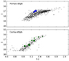 |
Fig. 1. Color–magnitude diagram (I, V − I) of the RGB of Fornax (top) and Carina (bottom). The V, I magnitudes are from ESO 2.2 m WFI (Battaglia et al. 2006; Starkenburg et al. 2010). The gray dots are probable Fornax and Carina members based on their radial velocities (Starkenburg et al. 2010). The colored points are stars with [Fe/H] ≤ –2.5 and more than five chemical abundances measured. The large blue and green circles show respectively the Fornax and Carina stars analyzed here. Data shown from other works are Tafelmeyer et al. (2010) (small blue square); Venn et al. (2012) (small green squares); and Susmitha et al. (2017) (small green star). |
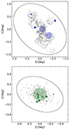 |
Fig. 2. Spatial distribution of stars. Top panel: Fornax stars, the large shaded blue circles correspond to the VLT/FLAMES observations of Letarte et al. (2010) (upper) and of Lemasle et al. (2014) (lower). Bottom panel: Carina stars. The large shaded green circle corresponds to the VLT/FLAMES observations of Lemasle et al. (2012), the green triangles are from Koch et al. (2008); the other symbols are same as in Fig. 1. The ellipses indicate the tidal radius of Fornax and Carina, respectively. |
Observation journal.
The two EMP candidates in Fornax, fnx_06_019 and fnx0579x−1, were sufficiently bright to enable follow-up at high resolution with the UVES spectrograph (Dekker et al. 2000) mounted at the ESO VLT (program ID 0100.D-0820(A)). We used dichroic 1 with the CCD#2 centered at 3900 Å and the CCD#3 centered at 5800 Å. Setting the slit width at 1.2″ led to a nominal resolution of R ∼ 34 000. The full wavelength coverage is ∼3200–6800 Å (see Table 1 for details), and the effective usable spectral information starts from ∼3800 Å due to the lower signal-to-noise ratio (S/N) toward the blue part of the spectrum. Each star was observed for a total of five hours, split into six individual sub-exposures. The final S/N ranges from 12 (blue part) to 45 (red part).
The four EMP candidates in Carina (LG04c_0008, Car1_t200, Car1_t174, and Car1_t194) were observed (program ID 094.D–0853(B)) with X-shooter (Vernet et al. 2011). The UVB slit was open to 0.8 × 11 arcsec2, while the VIS slit was open to 0.9 × 11 arcsec2, which led to a nominal resolution of R ∼ 6200 and R ∼ 7400, respectively. The total exposure time, in STARE mode, was 2.5 h for LG04c_0008 and 3 h for the other stars divided in 3 and 4 OBs of ∼3000 s, respectively. The usable wavelength range spans 3040–6800 Å with S/N ranging from ∼24 to ∼40.
In all cases the reduced data, including bias subtraction, flat fielding, wavelength calibration, spectral extraction, and order merging, were taken from the ESO Science Archive Facility. Table 1 provides the coordinates of our targets, the signal-to-noise ratios, and the radial velocities as measured in each wavelength interval. Table 2 lists the optical and near-infrared magnitudes of our sample. Figure 1 shows the color–magnitude diagram (CMD) of the targets, and Fig. 2 indicates the spatial location of our targets relative to the position of other spectroscopic studies in Carina and Fornax.
Optical and near-IR photometry.
2.2. Radial velocity measurements and normalization
The stellar heliocentric radial velocities (RVs) were measured with the IRAF1 task rvidlines on each individual exposure. The final RV is the average of these individual values weighted by their uncertainties. This approach allows us to detect possible binary stars, at least those whose RV variations can be detected within about one year. We did not find any evidence for binarity. After they were corrected for RV shifts, the individual exposures were combined into a single spectrum using the IRAF task scombine with a 2–3σ clipping. As a final step, each spectrum was visually examined, and the few remaining cosmic rays were removed with the splot routine.
The mean RV of each Fornax star (Table 1) coincides with the RV of Fornax, 54.1 ± 0.5 km s−1, within the velocity dispersion σ = 13.7 ± 0.4 km s−1 measured by Battaglia et al. (2006), and 55.46 ± 0.63 km s−1, within the velocity dispersion σ = 11.62 ± 0.45 km s−1 measured by Hendricks et al. (2014a). Similarly, the RVs of the Carina stars fall within the mean of the galaxy, 224.4 ± 5.95 km s−1 measured by Lemasle et al. (2012), and 223.9 km s−1 with σ = 7.5 km s−1 measured by Koch et al. (2006). This confirms that our stars are galaxy members. The spectra were normalized using DAOSPEC (Stetson & Pancino 2008) for each of the wavelength ranges presented in Table 1. We used a 20–40° polynomial fit.
3. Stellar model determination and chemical analysis
3.1. Line list and model atmospheres
Our line list combines those of Jablonka et al. (2015), Tafelmeyer et al. (2010), and Van der Swaelmen et al. (2013). Information on the spectral lines was taken from the VALD database (Piskunov et al. 1995; Ryabchikova et al. 1997; Kupka et al. 1999, 2000). The corresponding central wavelengths and oscillator strengths are given in Table A.1.
We adopted the new MARCS 1D atmosphere models and selected the Standard composition class, that is, we included the classical α-enhancement of +0.4 dex at low metallicity. They were downloaded from the MARCS web site (Gustafsson et al. 2008), and interpolated using Thomas Masseron’s interpol_modeles code, which is available on the same web site2. Inside a cube of eight reference models, this code performs a linear interpolation on three given parameters: Teff, log g, and [Fe/H].
3.2. Photometric temperature and gravity
The atmospheric parameters were initially determined using photometric information, as reported in Table 2. The first approximated determination of the stellar effective temperature (Teff) was based on the V − I, V − J, V − H, and V − K color indices measured by Battaglia et al. (2006), and the J and Ks photometry was taken from the VISTA commissioning data, which were also calibrated onto the 2MASS photometric system. We assumed Av = 3.24 ⋅ EB − V (Cardelli et al. 1989) and EB − V = 0.03 for Fornax (Letarte et al. 2010), and EB − V = 0.061 for Carina (de Boer et al. 2014) for the reddening correction. The adopted photometric effective temperatures (Teff) are listed in Table 3. They correspond to the simple average of the four color temperatures derived from V − I, V − J, V − H, and V − K with the calibration of Ramírez & Meléndez (2005).
CaT metallicity estimates, and photometric and final spectroscopic parameters.
Because very few Fe II lines can be detected in our X-shooter spectra, the determination of surface gravities from the ionization balance of Fe I versus Fe II was not possible. Non-local thermodynamic equilibrium (NLTE) effects also play a role at extremely low metallicity, and impact the abundances of Fe I, with Δ(Fe II–Fe I) up to +0.20 dex at [Fe/H] = −3 (Mashonkina et al. 2017b), and thus surface gravities were determined from their relation with Teff,
 (1)
(1)
assuming log g⊙ = 4.44, Teff⊙ = 5790 K, and Mbol⊙ = 4.75 for the Sun. We adopted a stellar mass of 0.8 M⊙ and calculated the bolometric corrections using the Alonso et al. (1999) calibration, with a distance of d = 138 kpc (Battaglia et al. 2006) for Fornax and d = 106 kpc (de Boer et al. 2014) for Carina.
3.3. Final stellar parameters and abundance determinations
We determined the stellar chemical abundances via the measurement of the equivalent widths (EWs) or spectral synthesis of atomic transition lines when necessary (see below). Lines present in the spectra and in our line list were detected and their EWs measured with DAOSPEC (Stetson & Pancino 2008). This code performs a Gaussian fit of each individual line and measures its corresponding EW. Although DAOSPEC fits saturated Gaussians to strong lines, it cannot fit the wider Lorentz-like wings of the profile of very strong lines, in particular beyond 120 mÅ at very high resolution (Kirby & Cohen 2012). For some of the strongest lines in our spectra, we therefore derived the abundances by spectral synthesis. All other detected lines by DAOSPEC were also inspected visually and the measured EWs were rejected when too uncertain (for example in the case of upper limits the abundances were determined through spectral synthesis), or the lines were totally rejected when the continuum level was too uncertain.
The measured EWs are provided in Tables A.1 and A.3. The values in parentheses indicate that the corresponding abundances were derived by spectral synthesis. The abundance derivation from EWs and the spectral synthesis calculation were performed with the Turbospectrum code (Alvarez & Plez 1998; Plez 2012), which assumes local thermodynamic equilibrium (LTE), but treats continuum scattering in the source function. We used a plane-parallel transfer for the line computation; this is consistent with our previous work on EMP stars (Tafelmeyer et al. 2010; Jablonka et al. 2015; Lucchesi et al. 2020).
In order to derive the final Teff and the microturbulence velocities (vt), we checked or required no trend between the abundances derived from Fe I and excitation potential (χexc) or the predicted3 EWs. In order to minimize the NLTE effect on the measured abundances we excluded from the analysis Fe I lines with χexc < 1.4 eV. Furthermore, very strong lines (EW > 120 mÅ) with strong wings that cannot be well fit are also excluded.
Starting from the initial photometric parameters of Table 3, we adjusted Teff and vt by minimizing the slopes of the diagnostic plots, within its 2σ uncertainty. We did not force ionization equilibrium between Fe I and Fe II, taking into account that there will likely be NLTE effects at these low metallicities (Amarsi et al. 2016; Mashonkina et al. 2017b; Ezzeddine et al. 2017). For each iteration the corresponding values of log g were computed from its relation with Teff (Eq. (1)), assuming the updated values of Teff, and adjusting the model metallicity to the mean iron abundance derived in the previous iteration. The final values of Teff are less than 30 K away from the initial photometric estimates; the only exception is fnx0579x−1, which is 138 K cooler than the mean photometric temperature.
We derived the chemical abundances of blended lines, strong lines (EW > 100 mÅ), or upper limits (EW < 25 mÅ) by spectral synthesis. These abundances were obtained using our own code (as in Lucchesi et al. 2020, 2022), which performs a χ2-minimization between the observed spectral features and a grid of synthetic spectra calculated on the fly with Turbospectrum. A line of a chemical element X is synthesized in a wavelength range of ∼10 to ∼50 Å. It is optimized by varying its abundance in steps of 0.1 dex, from [X/Fe] = −2.0 dex to [X/Fe] = +2.0 dex. In the same way, the resolution of the synthetic spectra is optimized when needed. Starting from the nominal instrumental resolution, synthetic spectra can be convolved with a wide range of Gaussian widths for each abundance step. A second optimization, with abundance steps of 0.01 dex, is then performed in a smaller range around the minimum χ2 in order to refine the results. Similarly, the elements with a significant hyperfine structure (HFS; e.g., Sc, Mn, Co, and Ba) are determined by running Turbospectrum in its spectral synthesis mode in order to properly take into account blends and the HFS components in the abundance derivation, as in North et al. (2012) and Prochaska & McWilliam (2000) for Sc and Mn, and from the Kurucz web site4 for Co and Ba.
The final abundances are listed in Table A.4. The solar abundances are taken from Asplund et al. (2009).
3.4. Error budget
The uncertainties on the abundances were derived considering the uncertainties on the atmospheric parameters and on the EWs, in a procedure similar to that used in our other works (e.g., Tafelmeyer et al. 2010; Jablonka et al. 2015; Hill et al. 2019; Lucchesi et al. 2020).
Uncertainties due to the atmospheric parameters. To estimate the sensitivity of the derived abundances to the adopted atmospheric parameters, we repeated the abundance analysis and varied only one stellar atmospheric parameter at a time by its corresponding uncertainty, keeping the others fixed and repeating the analysis. The estimated internal errors are ±100 K in Teff, ±0.15 dex in log (g), and ±0.15 km s−1 in vt for the UVES sample, and ±150 K in Teff, ±0.15 dex in log (g) for the X-shooter sample. Because the S/N and atmospheric parameters of our sample stars are very close to each other, we estimated the typical errors considering a single reference star. Table 4 lists the effects of these changes on the derived abundances for fnx_06_019 in the UVES sample, and Table 5 lists the effects of these changes on the derived abundances for carLG04c_0008 in the X-shooter sample.
Changes in the mean abundances Δ[X/H] caused by a ±100 K change in Teff, a ±0.15 dex change in log (g), and a ±0.15 km s−1 change in vt for the UVES star fnx_06_019.
Changes in the mean abundances Δ[X/H] caused by a ±150 K change in Teff with consistent changes in photometric log (g) and vt, and by a change of ±0.15 dex in log (g) only, for the X-shooter star carLG04c_0008.
Uncertainties due to EWs or spectral fitting. The uncertainties on the individual EW measurements (δEWi) are provided by DAOSPEC (see Table A.1) and are computed according to the formula (Stetson & Pancino 2008)
 (2)
(2)
where Ip and δIp are respectively the intensity of the observed line profile at pixel p and its uncertainty, and ICp and δICp are the intensity and uncertainty of the corresponding continuum. The uncertainties on the intensities are estimated from the scatter of the residuals that remain after subtraction of the fitted line (or lines in the case of blends). The corresponding uncertainties σEWi on individual line abundances are propagated by Turbospectrum. This is a lower limit to the real EW error because systematic errors, such as the continuum placement, are not accounted for.
In order to account for additional sources of error, we quadratically added a 5% error to the EW uncertainty so that no EW has an error smaller than 5%. For the abundances derived by spectral synthesis (e.g., strong lines, hyperfine structure, or carbon from the G band), the uncertainties were visually estimated by gradually changing the parameters of the synthesis until the deviation from the observed line became noticeable. The abundance uncertainty for an element X due to the individual EW uncertainties (σEWi propagated from δEWi) are computed as
 (3)
(3)
where NX represents the number of lines measured for element X. The dispersion σX around the mean abundance of an element X measured from several lines is computed as
 (4)
(4)
where ϵ stands for the logarithmic abundance.
The final error on the elemental abundances is defined as σfin = max(σEW(X),  ,
,  ). As a consequence, no element X can have an estimated uncertainty σX < σFe; this is particularly important for species for which the abundances are derived on very few lines.
3.5. Specific comments on abundance determinations
3.5.1. Carbon
Carbon abundances were determined by spectral synthesis of the region of the CH molecular G-band. The carbon abundances of the UVES Fornax sample were determined in the deeper and unblended 4222–4225 Å region, while carbon was determined in a larger range of the CH molecular band, between 4270 Å and 4330 Å for the X-shooter sample in Carina. We assumed [O/Fe] = [Mg/Fe], but since the carbon abundance is low in our sample stars, the exact [O/Fe] assumed has very little effect on our results. The CH molecular band is shown in Fig. 3 for the X-shooter spectra of our four Carina stars.
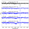 |
Fig. 3. X-shooter spectra of the four Carina stars (blue) in the region of the CH absorption, from the most metal poor at the top ([Fe/H] = −3.03) to the most metal rich at the bottom ([Fe/H] = −2.58). For comparison the spectrum of the Sculptor star Scl074_02 (black, at the top) is shown, with similar atmospheric parameters ([Fe/H] = −3.0) from Starkenburg et al. (2013). |
3.5.2. Lithium
Unfortunately, the Li resonance doublet at 6707 Å was not measurable in any of our stars at our available quality of the UVES or X-shooter spectra. This was expected, since Li on the surface of RGB stars is typically depleted due to dredge-up and mixing (e.g., Gratton et al. 2000; Lind et al. 2009). None of our target stars are therefore lithium-enhanced giants, which have been found in small fractions in most types of environments, including dwarf galaxies (e.g., Kirby et al. 2012; Hill et al. 2019).
3.5.3. Sodium and aluminium
The sodium was measured from the two 5889.951 Å and 5895.924 Å resonance lines through spectral synthesis. The X-shooter spectra of the four Carina target stars are presented in the region of the Na lines and the CH absorption in Figs. 4 and 3, respectively. They are compared to a star from Starkenburg et al. (2013) in the Sculptor dSph galaxy, Scl074_02, with very similar atmospheric parameters (Teff = 4595 K log g = 1.21 [Fe/H] = –3.0 vt = 2.1 km s−1), but significantly lower Na. The carbon abundance is very similar in all stars shown in Fig. 3, with low [C/Fe] ≤ –0.5. However, the difference can be clearly seen in the sodium region (Fig. 4), where the sodium lines appear stronger in Carina than in Sculptor. We note that interstellar Na lines are observed at different radial velocities and are unlikely to be contaminating the measured lines.
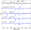 |
Fig. 4. X-shooter spectra of the four Carina stars (blue) in the region of the Na I doublet, from the most metal poor at the top ([Fe/H] = −3.03) to the most metal rich at the bottom ([Fe/H] = −2.58), and the spectrum of the Sculptor star Scl074_02 (black, at the top) with similar atmospheric parameters ([Fe/H] = −3.0) from Starkenburg et al. (2013). |
Two Al I lines are detected in the UVES spectra, but they are in a noisy part of the spectrum and fall very close to the strong Ca II H & K absorption doublet. Furthermore, the continuum level is hard to determine in this region, and the derived abundances strongly depend on it. Because of these difficulties, Al was only derived for one star, fnx_06_019, based on one line at 3961.52 Å.
3.5.4. α-elements
Magnesium. The UVES Mg abundances are based on three lines. Two of them are rather strong (5172.684 and 5183.604 Å), with EW > 100 mÅ and have non-Gaussian line profiles. The abundances of these lines are not consistent with the weaker 5528.405 Å line. For this reason, we derived the Mg abundance through spectral synthesis, after which all lines had consistent abundances. Three additional Mg I lines (4167.271, 4351.906, and 5711.088 Å) were detected in our spectra, but were discarded because too noisy, strongly blended, and too weak, respectively. The Mg abundances from the X-shooter sample were obtained through spectral synthesis in two 20 Å windows, one centered on the 5172.684 Å line, taking into account the blends at the X-shooter resolution, and one centered on the 5183.604 Å line.
Silicon. One Si I line was detected in our UVES spectra, at 4102.936 Å, but in a noisy part of the spectrum; it falls close to the strong Hδ absorption line. However, we were able to derive a Si abundance in both Fornax stars based on this one line.
Calcium. Three Ca I lines were used in the X-shooter spectra for the Carina stars. Calcium was not measurable in the star car1_t200. In the Fornax sample, in the red part of the UVES spectra (> 5500 Å ) 6 and 11 clean Ca I lines were used, for fnx0579x-1 and fnx_06_019, respectively. Examples of the Ca I lines for fnx_06_019 are shown in Fig. 5.
 |
Fig. 5. Examples of the Ca I lines used in the UVES spectrum (black) for the Fornax star fnx_06_019. In blue is the EW fitting from DAOSPEC. Atomic data for each line is listed in the panels, along with the derived abundances, which agree very well between different lines. |
Titanium. The Ti I abundances are based on 10−11 lines, all giving consistent abundance values from their EW. The Ti II abundances are based on 8–14 lines. They are slightly more scattered as many of them are rather strong. The mean abundances of Ti I and Ti II are different by Δ(Ti II−Ti I) = +0.50. This is explained by the fact that Ti II is less sensitive to NLTE effects than its neutral state. Thus, following Jablonka et al. (2015), for the purpose of our discussion we adopted the Ti II abundances as the most representative of the Titanium content in our stars.
3.5.5. Iron-peak elements
Chromium. Cr abundances were derived from 4 to 5 Cr I lines in the red part of the UVES spectra; all of them give consistent results from their EWs. Five extra lines were detected in our spectra (4254.352, 4274.812, 4289.73, 5206.023, and 5208.409 Å), but they were rejected for being too strong (> 110 mÅ) or too noisy. In the X-shooter spectra only the strongest λ5206.023 and 5208.409 Å lines were accessible. Cr abundances were obtained from a single spectral synthesis in a 20 Å wavelength range covering the two lines and taking into account the blends at this resolution.
Manganese. Mn abundances rely on the three Mn I 4030.75 Å, 4033.06 Å, and 4034.48 Å lines. These were synthesized taking into account their HFS components and give consistent abundance results. The Mn lines 4041.35 Å and 4823.52 Å are also present in our spectra, but they are weak (∼30 mÅ) and too affected by noise, and were thus discarded. In the case of X-shooter spectra, a single spectral synthesis was done in a 20 Å window centered on the Mn triplet.
3.5.6. Neutron-capture elements
Strontium. Three Sr II lines are present in our spectra (4077.709, 4161.792, and 4215.519 Å). While the 4215.519 Å line was the most reliable in the UVES spectra, the 4077.709 Å line was less affected by blends and better suited for the X-shooter spectra.
Barium. Ba abundances were measured from two to four lines (4554.029, 4934.076, 5853.668, 6141.713, and 6496.897 Å) in the UVES and X-shooter spectra by spectral synthesis taking into account blends and HFS.
Additional neutron-capture elements were measurable in the spectrum of the r-process rich star fnx_06_019 in Fornax. Figure 6 compares two UVES spectra in the region of the lanthanum and europium lines, showing a clear neutron-capture enhancement in fnx_06_019 (see also Fig. B.1).
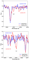 |
Fig. 6. Two UVES spectra in the region of the lanthanum (top) and europium (bottom) lines. In red is the r-process rich star fnx_06_019, and in blue the r-process normal star fnx0579x−1. |
Lanthanum. The La abundance was determined from the λ4920.98 Å line, which is the reddest available La II line and the least affected by noise.
The detection was checked by computing synthetic spectra for the 4077.34, 4086.71, and 4123.23 Å lines using the abundance derived from the 4920.98 Å line (Fig. B.1). All the lines were in good agreement with the adopted abundance.
Neodymium. The Nd abundance was determined from the two clean and unblended Nd II lines at 4825.48 and 5319.81 Å, and further confirmed to be consistent with the 4109.45 and 4061.08 Å lines.
Dysprosium. The abundance was measured from the Dy II 4103.31 Å line by spectral synthesis. The 3944.68 Å line is too affected by noise and continuum level uncertainty, while the 4449.7 Å line is too strongly blended to be reliable.
4. Results
The measured LTE chemical abundances for our four Carina, and two Fornax stars are listed in Table A.4 and shown in Figs. 7–13. The different element groups are discussed in the following sections.
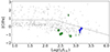 |
Fig. 7. [C/Fe] as a function of log (L/L⊙) for Fornax (blue) and Carina (green). The circles are data from this work. The green upper limits are from Venn et al. (2012), and the green star is a CEMP-no star from Susmitha et al. (2017). The blue square is the Fornax member from Tafelmeyer et al. (2010). The gray dots are MW halo stars (Placco et al. 2014). The dotted line traces the criterion of Aoki et al. (2007b) to define C-enhanced stars, which takes into account the depletion of carbon along the RGB. Only stars with [Fe/H] < –2.5 are included. |
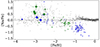 |
Fig. 8. LTE Sodium-to-iron ratios as a function of [Fe/H] are shown for stars in the Fornax and Carina dSph galaxies, and in the MW. Fornax members are in blue: large circles are from this work; small circles are from Lemasle et al. (2014); small triangles are from Letarte et al. (2010); small stars are members of Fornax globular clusters 1, 2, and 3 from Letarte et al. (2006). The square at [Fe/H] = –3.66 is an EMP star from Tafelmeyer et al. (2010). Carina members are in green: large circles are from this work; small triangles are from Koch et al. (2008); small circles are from Norris et al. (2017); small squares are from Venn et al. (2012); the star is a CEMP-no from Susmitha et al. (2017). The gray dots are MW stars (Bensby et al. 2014; Yong et al. 2013; Frebel et al. 2010). |
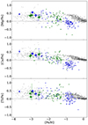 |
Fig. 9. Abundance ratios for the α-elements Mg, Ca, and Ti (from top to bottom) as a function of [Fe/H]. The symbols are the same as in Fig. 8. |
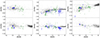 |
Fig. 10. Iron-peak elements as a function of [Fe/H]. From left to right, top to bottom: [Sc/Fe], [Cr/Fe], [Mn/Fe], [Co/Fe], [Ni/Fe], and [Zn/Fe] for metal-poor stars in Fornax, Carina, and MW. The symbols are the same as in Fig. 8. The stars studied in this paper are the large circles. The MW data are from Bensby et al. (2014), Yong et al. (2013), and Frebel et al. (2010). |
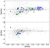 |
Fig. 11. Neutron-capture elements. Shown are the barium-to-iron ratio (top) and strontium-to-iron ratio (bottom) as a function of [Fe/H] in Fornax (blue) and Carina (green), compared to MW stars (gray) from Roederer (2013). The symbols are the same as in Fig. 8; the large circles represent the new sample analyzed here. |
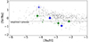 |
Fig. 12. Barium-to-strontium ratio as a function of [Ba/H]. The references are the same as in Fig. 11. The empirical r-process limit is shown as a dashed line (Mashonkina et al. 2017a). |
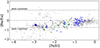 |
Fig. 13. Barium-to-europium ratio as a function of [Fe/H]. The symbols are the same as in Fig. 11. The MW stars are from Frebel et al. (2010), and Venn et al. (2004). The limits of pure s-process and r-process are shown as dashed lines (Mashonkina et al. 2017a). |
4.1. Literature comparison samples
In Figs. 7–13, the abundances from the Milky Way are shown as gray dots and are compiled from Placco et al. (2014) for carbon; from Bensby et al. (2014), and Yong et al. (2013) for Na, Mg, Ca, Ti; and from Frebel et al. (2010) for Na. The Milky Way iron-peak elements (Sc, Cr, Mn, Co, Ni, Zn) are from Bensby et al. (2014), Yong et al. (2013), and Frebel et al. (2010); while the abundances of the neutron-capture elements strontium and barium are from Roederer (2013). The Milky Way europium abundances are from Frebel et al. (2010), and Venn et al. (2004).
Abundances measured in Carina are from Koch et al. (2008), Venn et al. (2012), and Norris et al. (2017). Norris et al. (2017) compiled 63 RGB stars, of which 14 stars were totally new observations, while 18 stars were re-observations and 31 stars were re-analyses of stars initially studied by Lemasle et al. (2012), Shetrone et al. (2003), and Venn et al. (2012). For the purpose of homogeneity we show the Norris et al. (2017) results and refer to this paper for a detailed description of the individual samples. The only exception is made for the Venn et al. (2012) sample. Since their work includes more chemical elements than Norris et al. (2017), we kept the original results of the nine Carina members from Venn et al. (2012). The Fornax comparison samples are taken from Letarte et al. (2006, 2010), Lemasle et al. (2014), and Tafelmeyer et al. (2010).
4.2. Carbon
Figure 7 presents the carbon abundances measured in Fornax and Carina at [Fe/H] < −2.5, compared to the literature data. The four Carina stars analyzed in this paper all present very low carbon levels, similar to the upper limits derived in the Carina sample of Venn et al. (2012). The Carina [C/Fe] distribution is located at the lower edge of the Milky Way abundances, making Carina noticeably C-poor (see Fig. 3). However, we note that two CEMP-no stars have been identified in Carina, first in Susmitha et al. (2017) and more recently in Hansen et al. (2023).
In Fornax, our two stars and the one star previously studied by Tafelmeyer et al. (2010) have similar carbon-normal abundances. On average the Fornax stars are somewhat higher in C compared to Carina, especially when corrections for evolutionary status are taken into account.
We note that none of our six new stars is enhanced in carbon, while in the Milky Way the typical fraction of CEMP-no stars is ≈40% at [Fe/H] < –3 (Placco et al. 2014). This adds to previous results, showing that dSph galaxies are poor in CEMP-no stars relative to the Milky Way and the UFDs (Starkenburg et al. 2013; Skúladóttir et al. 2015, 2021, 2023; Jablonka et al. 2015; Simon et al. 2015; Kirby et al. 2015; Hansen et al. 2018; Lucchesi et al. 2020), for a more detailed discussion on this see Sect. 5.
4.3. Light element: Sodium
The LTE abundances of sodium are presented in Fig. 8. The Milky Way has a very large scatter in [Na/Fe] at low [Fe/H] < −2, and our new data points fall within this range. Fornax shows a near solar [Na/Fe] ≈ 0; instead, all four stars in Carina have high [Na/Fe] ≳ +0.5. Since direct comparison between the Carina (X-shooter) and Fornax (UVES) spectra is not meaningful, in Fig. 4 we plot the Na lines of the Carina stars together with an X-shooter spectrum of a Na-poor star in Sculptor. This comparison clearly shows the Carina stars to be Na rich.
Non-LTE effects can play an important role in the derived sodium abundances. The resonance lines, 5889.951 Å and 5895.924 Å, are especially sensitive. Very limited NLTE abundances are available in the literature. The apparent large dispersion at [Fe/H] < –2 could probably be significantly reduced if NLTE corrections were applied. We used the INSPECT database5 to compute corrections for our stars to investigate whether the [Na/Fe] difference between Fornax and Carina would remain (see Table A.2). The correction depends both on the measured LTE sodium abundances and on the metallicity and the stellar atmospheric parameters. The corrections for Carina were ⟨Δ[Na/Fe]NLTE⟩= − 0.33 and for Fornax ⟨Δ[Na/Fe]NLTE⟩= − 0.16. However, the Carina NLTE abundances are still higher, with ⟨[Na/Fe]NLTE⟩= + 0.37 ± 0.17; for Fornax ⟨[Na/Fe]NLTE⟩= − 0.06 ± 0.14.
The interpretation of this Na-enhancement is not straightforward. Norris et al. (2013) found that CEMP-no stars were likely to be enhanced in Na; however, the Carina stars are depleted in carbon (see the previous section, and Fig. 7). The origin of this Na enhancement, compared to other dSph galaxies, therefore remains unclear. We note however that there are two stars from Venn et al. (2012) with lower Na, so it seems that there is a significant scatter of Na in Carina, similar to the Milky Way.
4.4. αa-elements
The chemical abundances of the α-elements Mg and Ca, together with Ti, are shown in Fig. 9. All three elements show a very similar trend of enhanced [α/Fe] ≈ + 0.4 at [Fe/H] < –2.5 in all our literature samples, and in Hendricks et al. (2014b) who focuses on determining the position of the α-knee in Fornax. Our results are in perfect agreement with the Milky Way, and other dwarf galaxies, both the dSph galaxies (e.g., Tafelmeyer et al. 2010; Lucchesi et al. 2020; Theler et al. 2020) and the UFDs (e.g., Simon 2019).
The Carina dSph galaxy has a complex star formation history (e.g., Tolstoy et al. 2009; de Boer et al. 2014), and the scatter of [Mg/Fe] at intermediate metallicities, –2.5 < [Fe/H] < –1, is quite large, σ = 0.30 dex. However, the scatter seems to be reduced at [Fe/H] ≤ –2.5, where all stars are consistent with the same [Mg/Fe] value, σ = 0.08 dex. It is therefore possible that these low metallicities probe only the first star formation burst in Carina.
4.5. Iron-peak elements
Figure 10 presents Sc, Cr, Mn, Co, Ni, and Zn trends with Fe in Carina and Fornax, compared with the Milky Way halo and disk populations. The element Sc could be determined only in our Fornax sample, which had high-resolution UVES spectra. The production of Sc is dominated by core-collapse supernovae (ccSNe; Woosley et al. 2002; Battistini & Bensby 2015), and therefore, as expected, [Sc/Fe] is at the same level as the α-elements seen in Fig. 9.
For both Fornax and Carina, Cr and Mn closely follow the Milky Way trends at [Fe/H] < –2.5, as derived from 1D LTE methods. NLTE calculations for the neutral species of these elements show an overionization, leading to weakened lines and positive NLTE abundance corrections (Bergemann et al. 2019). Therefore, the increasing trends of [Cr/Fe] and [Mn/Fe] with [Fe/H] might be artificial. In the case of Co, our measurements are lower than the average trend in the Milky Way. Similarly, the Co abundances in the Sculptor dSph galaxy are low at [Fe/H] < –2.5 (Skúladóttir et al. 2024).
Nickel can be produced in ccSNe, and in thermonuclear Type Ia supernovae (SNIa; e.g., Jerkstrand 2018). Before SNIa start to dominate, [Fe/H] < –2, our sample definitely set the level at solar value, [Ni/Fe] ≈ 0, for both Carina and Fornax, implying that the global production of nickel follows that of iron in core-collapse supernovae. This is in excellent agreement with the Sculptor dSph galaxy and UFDs (Skúladóttir et al. 2024). However, subsolar [Ni/Fe] has been noted in the Fornax population at [Fe/H] > –1.2 (Letarte et al. 2010; Lemasle et al. 2014), and in Carina at [Fe/H] > –1.5 (Norris et al. 2017). This clearly corresponds to a stage of the galaxy chemical evolution when the ejecta of SNIa dominate the composition of the interstellar medium. Similar results are found in other dSph galaxies (Hill et al. 2019; Kirby et al. 2019; Theler et al. 2020), as well as accreted dwarf galaxies (e.g., Nissen & Schuster 2010).
There is a known increase in [Zn/Fe] toward low [Fe/H] (e.g., Cayrel et al. 2004) (see Fig. 10, bottom right). The NLTE corrections of Zn (Takeda et al. 2005) are small in the metal-poor regime and do not fully explain this trend, and it remains poorly understood. We were only able to measure Zn for the star fnx_06_019, which falls on the Milky Way halo trend at [Zn/Fe] = +0.29, comparable to the level of the [α/Fe] plateau. This was also observed in two Sextans EMP stars (Lucchesi et al. 2020), two stars in Ursa Minor (Cohen & Huang 2010), and in Sculptor (Skúladóttir et al. 2017, 2024), highlighting the role of ccSNe in the production of zinc in the early stage of galaxy evolution.
4.6. Neutron-capture elements
Figure 11 shows our measurements of [Sr/Fe] and [Ba/Fe] with [Fe/H]. The Ba and Sr abundances of our sample stars are consistent with the large spread in the Milky Way. The abundance ratio of [Sr/Ba] with [Ba/H] is presented in Fig. 12. The [Sr/Ba] ratios of the Fornax stars are compatible with those of the Milky Way. However, these ratios in the Carina dSph galaxy are somewhat lower. Mashonkina et al. (2017a) identified two populations in [Sr/Ba], one with a trend similar to that found in the Milky Way (and Fornax), increasing toward low [Ba/H], and the other of near constant [Sr/Ba], similar to the empirical r-process ratio. The Carina abundances seem to fall between these two populations.
Only in the r-I star, fnx_06_019, were we able to measure [Eu/Fe]. Its [Ba/Eu] = –0.5 value sits just above the pure r-process ratio, as is shown in Fig. 13. This star, therefore, likely also shows some minor s-process contribution, which is evident from its rather high [Sr/Ba] = +0.5 (see Fig. 12). Not only is this star rich in Eu, but it is also enhanced in La, Nd, and Dy, as is evident from the very strong lines shown in Fig. B.1 and listed Table A.4. However, we note that the light neutron-capture elements, Sr, Y, and Zr, are not enhanced: [Sr/Fe] = –0.62, [Y/Fe] = –0.15, [Zr/Fe] = +0.22. The elements Y, Sr, and Zr have a similar origin, and their ratios are observed to be approximately constant in the Milky Way halo (François et al. 2007).
This is the first r-I star identified in a dSph galaxy at such low [Fe/H]. The r-I and r-II stars discovered in dSph galaxies to date seem to cover the more metal-rich end of the metallicity distribution compared to halo r-I stars (e.g., Shetrone et al. 2001; Aoki et al. 2007b; Cohen & Huang 2009; Hansen et al. 2018; Reichert et al. 2020).
5. Discussion and conclusions
Here we follow-up some of the first EMP candidates in the Fornax and Carina dSph galaxies to populate the as-yet-uncovered metallicity range –3.1 ≤ [Fe/H] ≤ –2.5. It is now clear that regardless of the subsequent evolution of the local classical dwarf galaxies, which harbor very different star formation histories, the first generations of stars formed in very similar way in these systems. Almost all the chemical elements follow the same trend with (low) metallicity, and match the known relations for our Galaxy.
However, there are clear differences in the [C/Fe] abundances of dSph galaxies, compared to UFDs and the Milky Way. In Fig. 14 we compare the cumulative fraction of CEMP-no stars in dSph galaxies to that of the Milky Way, as Ji et al. (2020) did for UFDs. We used all the available literature data, corrected for carbon depletion due to stellar evolution (Placco et al. 2014)6, that had minimal or no selection effects in regards to C-abundance. In particular, we were unable to include Hansen et al. (2023), as they specifically targeted CEMP stars, thus not providing information about the CEMP-no fraction. No CEMP-s stars (i.e. CEMP stars presenting s-process enhancement, [Ba/Fe] > 0) were included; however, we did include the [Fe/H] = –3.38 star in Canes Venatici I, without a Ba measurement, which Yoon et al. (2020) claimed was a CEMP-no star, using the stars position in the [Fe/H]-A(C) diagram. We note that [C/Fe] in this star is ≳1 dex higher than all other dSph stars found in the literature. From Fig. 14 it is evident that the CEMP-no fraction in dSph galaxies is significantly lower than in the Milky Way, reaching fractions of ≈6% at [Fe/H] < –2, based on 15 CEMP-no stars, out of 251 in total. At the lowest metallicities, [Fe/H] ≤ –3.4, none of the seven known stars in dSph galaxies is C-enhanced, while the CEMP-no fraction in the Milky Way at these metallicities is > 50%. This also implies a discrepancy in the CEMP-no fraction of dSph galaxies and UFDs, since the latter are in agreement with the Milky Way fraction (e.g., Ji et al. 2020). Our findings therefore confirm what has previously been stated with more limited data (e.g., Starkenburg et al. 2013; Skúladóttir et al. 2015, 2024; Lucchesi et al. 2020).
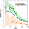 |
Fig. 14. Cumulative fraction of CEMP-no stars ([C/Fe] ≥ +0.7) observed in dSph galaxies (orange solid line) with the associated 1σ 84.13% confidence level (Gehrels 1986) (orange shaded area). Fraction in the MW halo (blue solid line) is from Placco et al. (2014), while the fraction computed by Ji et al. (2019) in UFDs is represented by the green solid line with its associated uncertainty (green shaded area). The carbon abundances in dSph galaxies are corrected for internal mixing (Placco et al. 2014) and are compiled from these works: Lucchesi et al. (2020), Jablonka et al. (2015), Tafelmeyer et al. (2010), Skúladóttir et al. (2015, 2024), Kirby et al. (2015), Venn et al. (2012), Starkenburg et al. (2013), Susmitha et al. (2017), Hansen et al. (2018), Yoon et al. (2020), Kirby & Cohen (2012). |
We see differences in the Na abundances of Fornax and Carina, where all four stars in the Carina dSph galaxy are high in [Na/Fe]LTE ≳ +0.5 (see Fig. 8). This is puzzling since high Na abundances are typically found in CEMP-no stars (e.g., Norris et al. 2013), and are predicted by their theoretical yields (e.g., Heger & Woosley 2002), but the Carina stars all have low [C/Fe] < 0. Furthermore, this is typically not seen in other very metal-poor stars in dSph galaxies (Tafelmeyer et al. 2010; Jablonka et al. 2015; Skúladóttir et al. 2024).
As we do in the Milky Way, at low [Fe/H] ≲ –2.5 we find a large scatter of the neutron-capture elements in both the Carina and the Fornax dSph galaxies. We report the discovery of a Eu-rich, r-I star in Fornax: [Eu/Fe] = +0.8 and [Eu/Ba] = +0.5. This star, fnx_06_019, also shows an outstanding enrichment in La, Nd, and Dy ([X/Fe] > +0.5). This is the first such case for a C-normal star at such low metallicity ([Fe/H] = –2.92) in a classical dSph galaxy. This points to a prolific r-process event early in the history of the Fornax dSph galaxy, where r-process enhancements were previously only seen at higher [Fe/H] > − 2 (Letarte et al. 2010; Lemasle et al. 2014; Reichert et al. 2020, 2021).
The present analysis contributes to the limited understanding of the earliest chemical enrichment in dSph galaxies. To further investigate the range of abundance patterns observed in different systems, it is clear that more observations are needed. Fortunately, the situation will improve drastically with upcoming spectroscopic surveys, such as WEAVE (Jin et al. 2024) and 4MOST (de Jong et al. 2019), in particular the dedicated dwarf galaxy survey 4DWARFS (Skúladóttir et al. 2023). With large and homogeneous data sets we will be able to identify rare EMP stars, and better constrain the CEMP-no fraction in different galaxies. Furthermore, we will obtain detailed spatial information that will allow us to trace the individual events causing r-process enrichment. Our work serves to highlight that it is fundamental to study metal-poor stars in galaxies of different sizes and star formation histories to get a complete picture of the galaxy formation and first chemical enrichment.
Image Reduction and Analysis Facility; Astronomical Source Code Library [record ascl:http://www.ascl.net/9911.002].
According to Magain (1984), the use of observed EWs produce an increase in vt of 0.1–0.2 km s−1, which would be reflected in a decrease in the measured [Fe/H] values of a few hundredths of a dex in a systematic way. A variation like this does not change the results significantly.
Acknowledgments
We thank E. Tolstoy for useful comments and suggestions on the manuscript. R.L. and Á.S. have received funding from the European Research Council (ERC) under the European Union’s Horizon 2020 research and innovation programme (grant agreement No. 804240). D.M. gratefully acknowledges support from the ANID BASAL projects ACE210002 and FB210003, from Fondecyt Project No. 1220724, and from CNPq Project 350104/2022-0.
References
- Alonso, A., Arribas, S., & Martínez-Roger, C. 1999, A&AS, 140, 261 [NASA ADS] [CrossRef] [EDP Sciences] [Google Scholar]
- Alvarez, R., & Plez, B. 1998, A&A, 330, 1109 [NASA ADS] [Google Scholar]
- Amarsi, A. M., Lind, K., Asplund, M., Barklem, P. S., & Collet, R. 2016, MNRAS, 463, 1518 [NASA ADS] [CrossRef] [Google Scholar]
- Aoki, W., Honda, S., Sadakane, K., & Arimoto, N. 2007a, PASJ, 59, L15 [NASA ADS] [Google Scholar]
- Aoki, W., Beers, T. C., Christlieb, N., et al. 2007b, ApJ, 655, 492 [NASA ADS] [CrossRef] [Google Scholar]
- Aoki, W., Arimoto, N., Sadakane, K., et al. 2009, A&A, 502, 569 [NASA ADS] [CrossRef] [EDP Sciences] [Google Scholar]
- Asplund, M., Grevesse, N., Sauval, A. J., & Scott, P. 2009, ARA&A, 47, 481 [NASA ADS] [CrossRef] [Google Scholar]
- Barklem, P. S., Christlieb, N., Beers, T. C., et al. 2005, A&A, 439, 129 [NASA ADS] [CrossRef] [EDP Sciences] [Google Scholar]
- Battaglia, G., Tolstoy, E., Helmi, A., et al. 2006, A&A, 459, 423 [NASA ADS] [CrossRef] [EDP Sciences] [Google Scholar]
- Battistini, C., & Bensby, T. 2015, A&A, 577, A9 [NASA ADS] [CrossRef] [EDP Sciences] [Google Scholar]
- Beers, T. C., & Christlieb, N. 2005, ARA&A, 43, 531 [NASA ADS] [CrossRef] [Google Scholar]
- Bensby, T., Feltzing, S., & Oey, M. S. 2014, A&A, 562, A71 [NASA ADS] [CrossRef] [EDP Sciences] [Google Scholar]
- Bergemann, M., Gallagher, A. J., Eitner, P., et al. 2019, A&A, 631, A80 [NASA ADS] [CrossRef] [EDP Sciences] [Google Scholar]
- Bettinelli, M., Hidalgo, S. L., Cassisi, S., Aparicio, A., & Piotto, G. 2018, MNRAS, 476, 71 [NASA ADS] [CrossRef] [Google Scholar]
- Bettinelli, M., Hidalgo, S. L., Cassisi, S., et al. 2019, MNRAS, 487, 5862 [NASA ADS] [CrossRef] [Google Scholar]
- Cardelli, J. A., Clayton, G. C., & Mathis, J. S. 1989, ApJ, 345, 245 [Google Scholar]
- Cayrel, R., Depagne, E., Spite, M., et al. 2004, A&A, 416, 1117 [NASA ADS] [CrossRef] [EDP Sciences] [Google Scholar]
- Cohen, J. G., & Huang, W. 2009, ApJ, 701, 1053 [NASA ADS] [CrossRef] [Google Scholar]
- Cohen, J. G., & Huang, W. 2010, ApJ, 719, 931 [NASA ADS] [CrossRef] [Google Scholar]
- de Boer, T. J. L., Tolstoy, E., Hill, V., et al. 2012, A&A, 544, A73 [NASA ADS] [CrossRef] [EDP Sciences] [Google Scholar]
- de Boer, T. J. L., Tolstoy, E., Lemasle, B., et al. 2014, A&A, 572, A10 [NASA ADS] [CrossRef] [EDP Sciences] [Google Scholar]
- de Jong, R. S., Agertz, O., Berbel, A. A., et al. 2019, Messenger, 175, 3 [Google Scholar]
- Dekker, H., D’Odorico, S., Kaufer, A., Delabre, B., & Kotzlowski, H. 2000, in Proc. SPIE, eds. M. Iye, & A. F. Moorwood, SPIE Conf. Ser., 4008, 534 [NASA ADS] [CrossRef] [Google Scholar]
- Ezzeddine, R., Frebel, A., & Plez, B. 2017, ApJ, 847, 142 [Google Scholar]
- François, P., Depagne, E., Hill, V., et al. 2007, A&A, 476, 935 [Google Scholar]
- Frebel, A., Kirby, E. N., & Simon, J. D. 2010, Nature, 464, 72 [NASA ADS] [CrossRef] [Google Scholar]
- Gehrels, N. 1986, ApJ, 303, 336 [Google Scholar]
- Gratton, R. G., Sneden, C., Carretta, E., & Bragaglia, A. 2000, A&A, 354, 169 [NASA ADS] [Google Scholar]
- Gustafsson, B., Edvardsson, B., Eriksson, K., et al. 2008, A&A, 486, 951 [NASA ADS] [CrossRef] [EDP Sciences] [Google Scholar]
- Hansen, T. T., Simon, J. D., Marshall, J. L., et al. 2017, ApJ, 838, 44 [NASA ADS] [CrossRef] [Google Scholar]
- Hansen, C. J., El-Souri, M., Monaco, L., et al. 2018, ApJ, 855, 83 [NASA ADS] [CrossRef] [Google Scholar]
- Hansen, T. T., Simon, J. D., Li, T. S., et al. 2023, A&A, 674, A180 [NASA ADS] [CrossRef] [EDP Sciences] [Google Scholar]
- Heger, A., & Woosley, S. E. 2002, ApJ, 567, 532 [Google Scholar]
- Hendricks, B., Koch, A., Walker, M., et al. 2014a, A&A, 572, A82 [NASA ADS] [CrossRef] [EDP Sciences] [Google Scholar]
- Hendricks, B., Koch, A., Lanfranchi, G. A., et al. 2014b, ApJ, 785, 102 [NASA ADS] [CrossRef] [Google Scholar]
- Hill, V., Skúladóttir, Á., Tolstoy, E., et al. 2019, A&A, 626, A15 [NASA ADS] [CrossRef] [EDP Sciences] [Google Scholar]
- Hodge, P. W. 1961, AJ, 66, 83 [NASA ADS] [CrossRef] [Google Scholar]
- Jablonka, P., North, P., Mashonkina, L., et al. 2015, A&A, 583, A67 [NASA ADS] [CrossRef] [EDP Sciences] [Google Scholar]
- Jerkstrand, A. 2018, in 14th International Symposium on Origin of Matter and Evolution of Galaxies (OMEG 2017), AIP Conf. Ser., 1947, 020013 [Google Scholar]
- Ji, A. P., Frebel, A., Simon, J. D., & Chiti, A. 2016, ApJ, 830, 93 [NASA ADS] [CrossRef] [Google Scholar]
- Ji, A. P., Simon, J. D., Frebel, A., Venn, K. A., & Hansen, T. T. 2019, ApJ, 870, 83 [NASA ADS] [CrossRef] [Google Scholar]
- Ji, A. P., Li, T. S., Simon, J. D., et al. 2020, ApJ, 889, 27 [NASA ADS] [CrossRef] [Google Scholar]
- Jin, S., Trager, S. C., Dalton, G. B., et al. 2024, MNRAS, 530, 2688 [NASA ADS] [CrossRef] [Google Scholar]
- Kirby, E. N., & Cohen, J. G. 2012, AJ, 144, 168 [NASA ADS] [CrossRef] [Google Scholar]
- Kirby, E. N., Fu, X., Guhathakurta, P., & Deng, L. 2012, ApJ, 752, L16 [NASA ADS] [CrossRef] [Google Scholar]
- Kirby, E. N., Guo, M., Zhang, A. J., et al. 2015, ApJ, 801, 125 [NASA ADS] [CrossRef] [Google Scholar]
- Kirby, E. N., Xie, J. L., Guo, R., et al. 2019, ApJ, 881, 45 [NASA ADS] [CrossRef] [Google Scholar]
- Koch, A., Grebel, E. K., Wyse, R. F. G., et al. 2006, AJ, 131, 895 [Google Scholar]
- Koch, A., Grebel, E. K., Gilmore, G. F., et al. 2008, AJ, 135, 1580 [NASA ADS] [CrossRef] [Google Scholar]
- Koutsouridou, I., Salvadori, S., Skúladóttir, Á., et al. 2023, MNRAS, 525, 190 [NASA ADS] [CrossRef] [Google Scholar]
- Kupka, F., Piskunov, N., Ryabchikova, T. A., Stempels, H. C., & Weiss, W. W. 1999, A&AS, 138, 119 [NASA ADS] [CrossRef] [EDP Sciences] [Google Scholar]
- Kupka, F. G., Ryabchikova, T. A., Piskunov, N. E., Stempels, H. C., & Weiss, W. W. 2000, Balt. Astron., 9, 590 [Google Scholar]
- Lemasle, B., Hill, V., Tolstoy, E., et al. 2012, A&A, 538, A100 [NASA ADS] [CrossRef] [EDP Sciences] [Google Scholar]
- Lemasle, B., de Boer, T. J. L., Hill, V., et al. 2014, A&A, 572, A88 [NASA ADS] [CrossRef] [EDP Sciences] [Google Scholar]
- Letarte, B., Hill, V., Jablonka, P., et al. 2006, A&A, 453, 547 [NASA ADS] [CrossRef] [EDP Sciences] [Google Scholar]
- Letarte, B., Hill, V., Tolstoy, E., et al. 2010, A&A, 523, A17 [NASA ADS] [CrossRef] [EDP Sciences] [Google Scholar]
- Lind, K., Primas, F., Charbonnel, C., Grundahl, F., & Asplund, M. 2009, A&A, 503, 545 [NASA ADS] [CrossRef] [EDP Sciences] [Google Scholar]
- Lucchesi, R., Lardo, C., Primas, F., et al. 2020, A&A, 644, A75 [NASA ADS] [CrossRef] [EDP Sciences] [Google Scholar]
- Lucchesi, R., Lardo, C., Jablonka, P., et al. 2022, MNRAS, 511, 1004 [NASA ADS] [CrossRef] [Google Scholar]
- Magain, P. 1984, A&A, 134, 189 [NASA ADS] [Google Scholar]
- Mashonkina, L., Jablonka, P., Sitnova, T., Pakhomov, Y., & North, P. 2017a, A&A, 608, A89 [NASA ADS] [CrossRef] [EDP Sciences] [Google Scholar]
- Mashonkina, L., Jablonka, P., Pakhomov, Y., Sitnova, T., & North, P. 2017b, A&A, 604, A129 [NASA ADS] [CrossRef] [EDP Sciences] [Google Scholar]
- Nissen, P. E., & Schuster, W. J. 2010, A&A, 511, L10 [NASA ADS] [CrossRef] [EDP Sciences] [Google Scholar]
- Norris, J. E., Yong, D., Bessell, M. S., et al. 2013, ApJ, 762, 28 [NASA ADS] [CrossRef] [Google Scholar]
- Norris, J. E., Yong, D., Venn, K. A., et al. 2017, ApJS, 230, 28 [CrossRef] [Google Scholar]
- North, P., Cescutti, G., Jablonka, P., et al. 2012, A&A, 541, A45 [NASA ADS] [CrossRef] [EDP Sciences] [Google Scholar]
- Pace, A. B., Walker, M. G., Koposov, S. E., et al. 2021, ApJ, 923, 77 [NASA ADS] [CrossRef] [Google Scholar]
- Piskunov, N. E., Kupka, F., Ryabchikova, T. A., Weiss, W. W., & Jeffery, C. S. 1995, A&AS, 112, 525 [Google Scholar]
- Placco, V. M., Frebel, A., Beers, T. C., & Stancliffe, R. J. 2014, ApJ, 797, 21 [Google Scholar]
- Plez, B. 2012, Astrophysics Source Code Library [record ascl:1205.004] [Google Scholar]
- Prochaska, J. X., & McWilliam, A. 2000, ApJ, 537, L57 [Google Scholar]
- Ramírez, I., & Meléndez, J. 2005, ApJ, 626, 465 [Google Scholar]
- Reichert, M., Hansen, C. J., Hanke, M., et al. 2020, A&A, 641, A127 [NASA ADS] [CrossRef] [EDP Sciences] [Google Scholar]
- Reichert, M., Hansen, C. J., & Arcones, A. 2021, ApJ, 912, 157 [NASA ADS] [CrossRef] [Google Scholar]
- Roederer, I. U. 2013, AJ, 145, 26 [CrossRef] [Google Scholar]
- Ryabchikova, T. A., Piskunov, N. E., Kupka, F., & Weiss, W. W. 1997, Balt. Astron., 6, 244 [NASA ADS] [Google Scholar]
- Schatz, H., Becerril Reyes, A. D., Best, A., et al. 2022, J. Phys. G Nucl. Phys., 49, 110502 [NASA ADS] [CrossRef] [Google Scholar]
- Shetrone, M. D., Côté, P., & Sargent, W. L. W. 2001, ApJ, 548, 592 [NASA ADS] [CrossRef] [Google Scholar]
- Shetrone, M., Venn, K. A., Tolstoy, E., et al. 2003, AJ, 125, 684 [Google Scholar]
- Simon, J. D. 2019, ARA&A, 57, 375 [NASA ADS] [CrossRef] [Google Scholar]
- Simon, J. D., Jacobson, H. R., Frebel, A., et al. 2015, ApJ, 802, 93 [Google Scholar]
- Skúladóttir, Á., & Salvadori, S. 2020, A&A, 634, L2 [NASA ADS] [CrossRef] [EDP Sciences] [Google Scholar]
- Skúladóttir, Á., Tolstoy, E., Salvadori, S., et al. 2015, A&A, 574, A129 [NASA ADS] [CrossRef] [EDP Sciences] [Google Scholar]
- Skúladóttir, Á., Tolstoy, E., Salvadori, S., Hill, V., & Pettini, M. 2017, A&A, 606, A71 [NASA ADS] [CrossRef] [EDP Sciences] [Google Scholar]
- Skúladóttir, Á., Salvadori, S., Amarsi, A. M., et al. 2021, ApJ, 915, L30 [CrossRef] [Google Scholar]
- Skúladóttir, Á., Puls, A. A., Amarsi, A. M., et al. 2023, Messenger, 190, 19 [Google Scholar]
- Skúladóttir, Á., Vanni, I., Salvadori, S., & Lucchesi, R. 2024, A&A, 681, A44 [NASA ADS] [CrossRef] [EDP Sciences] [Google Scholar]
- Starkenburg, E., Hill, V., Tolstoy, E., et al. 2010, A&A, 513, A34 [CrossRef] [EDP Sciences] [Google Scholar]
- Starkenburg, E., Hill, V., Tolstoy, E., et al. 2013, A&A, 549, A88 [NASA ADS] [CrossRef] [EDP Sciences] [Google Scholar]
- Stetson, P. B., & Pancino, E. 2008, PASP, 120, 1332 [Google Scholar]
- Susmitha, A., Koch, A., & Sivarani, T. 2017, A&A, 606, A112 [NASA ADS] [CrossRef] [EDP Sciences] [Google Scholar]
- Tafelmeyer, M., Jablonka, P., Hill, V., et al. 2010, A&A, 524, A58 [CrossRef] [EDP Sciences] [Google Scholar]
- Takeda, Y., Hashimoto, O., Taguchi, H., et al. 2005, PASJ, 57, 751 [NASA ADS] [Google Scholar]
- Theler, R., Jablonka, P., Lucchesi, R., et al. 2020, A&A, 642, A176 [NASA ADS] [CrossRef] [EDP Sciences] [Google Scholar]
- Tolstoy, E., Hill, V., & Tosi, M. 2009, ARA&A, 47, 371 [Google Scholar]
- Van der Swaelmen, M., Hill, V., Primas, F., & Cole, A. A. 2013, A&A, 560, A44 [NASA ADS] [CrossRef] [EDP Sciences] [Google Scholar]
- Venn, K. A., Irwin, M., Shetrone, M. D., et al. 2004, AJ, 128, 1177 [NASA ADS] [CrossRef] [Google Scholar]
- Venn, K. A., Shetrone, M. D., Irwin, M. J., et al. 2012, ApJ, 751, 102 [Google Scholar]
- Vernet, J., Dekker, H., D’Odorico, S., et al. 2011, A&A, 536, A105 [NASA ADS] [CrossRef] [EDP Sciences] [Google Scholar]
- Wanajo, S., Sekiguchi, Y., Nishimura, N., et al. 2014, ApJ, 789, L39 [Google Scholar]
- Winteler, C., Käppeli, R., Perego, A., et al. 2012, ApJ, 750, L22 [Google Scholar]
- Woosley, S. E., Heger, A., & Weaver, T. A. 2002, Rev. Mod. Phys., 74, 1015 [NASA ADS] [CrossRef] [Google Scholar]
- Yong, D., Norris, J. E., Bessell, M. S., et al. 2013, ApJ, 762, 26 [Google Scholar]
- Yoon, J., Whitten, D. D., Beers, T. C., et al. 2020, ApJ, 894, 7 [Google Scholar]
Appendix A: Additional tables
Lines measured in the Fornax UVES spectra. Line parameters, observed EWs, and elemental abundances are provided. The EWs in brackets are given only as an estimation of the strength of the line. They should not be used to derive chemical abundances since most of them are blended, have large uncertainties, or derive from a Gaussian profile; the quoted abundances are derived through spectral synthesis for these lines.
Computed NLTE corrections for Na.
Lines measured in the Carina XSHOOTER spectra. Line parameters, observed EWs, and elemental abundances are provided. The EWs in brackets are given only as an indication; the quoted abundances are derived through spectral synthesis for these lines.
Derived LTE abundances for the Fornax stars observed with UVES and the Carina stars observed with X-SHOOTER, along with their associated errors (see § 3).
Appendix B: Measured lines of r-process elements
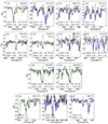 |
Fig. B.1. Individual lines of heavy (Z> 56) neutron-capture elements measured in the r-process rich star, fnx_06_019. From top to bottom: La II, Nd II, Eu II, and Dy II. The best fit synthetic spectra used for abundance determination are shown in green, while the synthetic spectra computed only to check agreement with other detected lines of lesser quality are in blue. The synthetic spectra computed without the element of interest, allowing the identification of blends, are in orange. |
All Tables
Changes in the mean abundances Δ[X/H] caused by a ±100 K change in Teff, a ±0.15 dex change in log (g), and a ±0.15 km s−1 change in vt for the UVES star fnx_06_019.
Changes in the mean abundances Δ[X/H] caused by a ±150 K change in Teff with consistent changes in photometric log (g) and vt, and by a change of ±0.15 dex in log (g) only, for the X-shooter star carLG04c_0008.
Lines measured in the Fornax UVES spectra. Line parameters, observed EWs, and elemental abundances are provided. The EWs in brackets are given only as an estimation of the strength of the line. They should not be used to derive chemical abundances since most of them are blended, have large uncertainties, or derive from a Gaussian profile; the quoted abundances are derived through spectral synthesis for these lines.
Lines measured in the Carina XSHOOTER spectra. Line parameters, observed EWs, and elemental abundances are provided. The EWs in brackets are given only as an indication; the quoted abundances are derived through spectral synthesis for these lines.
Derived LTE abundances for the Fornax stars observed with UVES and the Carina stars observed with X-SHOOTER, along with their associated errors (see § 3).
All Figures
|
Fig. 1. Color–magnitude diagram (I, V − I) of the RGB of Fornax (top) and Carina (bottom). The V, I magnitudes are from ESO 2.2 m WFI (Battaglia et al. 2006; Starkenburg et al. 2010). The gray dots are probable Fornax and Carina members based on their radial velocities (Starkenburg et al. 2010). The colored points are stars with [Fe/H] ≤ –2.5 and more than five chemical abundances measured. The large blue and green circles show respectively the Fornax and Carina stars analyzed here. Data shown from other works are Tafelmeyer et al. (2010) (small blue square); Venn et al. (2012) (small green squares); and Susmitha et al. (2017) (small green star). |
| In the text | |
|
Fig. 2. Spatial distribution of stars. Top panel: Fornax stars, the large shaded blue circles correspond to the VLT/FLAMES observations of Letarte et al. (2010) (upper) and of Lemasle et al. (2014) (lower). Bottom panel: Carina stars. The large shaded green circle corresponds to the VLT/FLAMES observations of Lemasle et al. (2012), the green triangles are from Koch et al. (2008); the other symbols are same as in Fig. 1. The ellipses indicate the tidal radius of Fornax and Carina, respectively. |
| In the text | |
|
Fig. 3. X-shooter spectra of the four Carina stars (blue) in the region of the CH absorption, from the most metal poor at the top ([Fe/H] = −3.03) to the most metal rich at the bottom ([Fe/H] = −2.58). For comparison the spectrum of the Sculptor star Scl074_02 (black, at the top) is shown, with similar atmospheric parameters ([Fe/H] = −3.0) from Starkenburg et al. (2013). |
| In the text | |
|
Fig. 4. X-shooter spectra of the four Carina stars (blue) in the region of the Na I doublet, from the most metal poor at the top ([Fe/H] = −3.03) to the most metal rich at the bottom ([Fe/H] = −2.58), and the spectrum of the Sculptor star Scl074_02 (black, at the top) with similar atmospheric parameters ([Fe/H] = −3.0) from Starkenburg et al. (2013). |
| In the text | |
|
Fig. 5. Examples of the Ca I lines used in the UVES spectrum (black) for the Fornax star fnx_06_019. In blue is the EW fitting from DAOSPEC. Atomic data for each line is listed in the panels, along with the derived abundances, which agree very well between different lines. |
| In the text | |
|
Fig. 6. Two UVES spectra in the region of the lanthanum (top) and europium (bottom) lines. In red is the r-process rich star fnx_06_019, and in blue the r-process normal star fnx0579x−1. |
| In the text | |
|
Fig. 7. [C/Fe] as a function of log (L/L⊙) for Fornax (blue) and Carina (green). The circles are data from this work. The green upper limits are from Venn et al. (2012), and the green star is a CEMP-no star from Susmitha et al. (2017). The blue square is the Fornax member from Tafelmeyer et al. (2010). The gray dots are MW halo stars (Placco et al. 2014). The dotted line traces the criterion of Aoki et al. (2007b) to define C-enhanced stars, which takes into account the depletion of carbon along the RGB. Only stars with [Fe/H] < –2.5 are included. |
| In the text | |
|
Fig. 8. LTE Sodium-to-iron ratios as a function of [Fe/H] are shown for stars in the Fornax and Carina dSph galaxies, and in the MW. Fornax members are in blue: large circles are from this work; small circles are from Lemasle et al. (2014); small triangles are from Letarte et al. (2010); small stars are members of Fornax globular clusters 1, 2, and 3 from Letarte et al. (2006). The square at [Fe/H] = –3.66 is an EMP star from Tafelmeyer et al. (2010). Carina members are in green: large circles are from this work; small triangles are from Koch et al. (2008); small circles are from Norris et al. (2017); small squares are from Venn et al. (2012); the star is a CEMP-no from Susmitha et al. (2017). The gray dots are MW stars (Bensby et al. 2014; Yong et al. 2013; Frebel et al. 2010). |
| In the text | |
|
Fig. 9. Abundance ratios for the α-elements Mg, Ca, and Ti (from top to bottom) as a function of [Fe/H]. The symbols are the same as in Fig. 8. |
| In the text | |
|
Fig. 10. Iron-peak elements as a function of [Fe/H]. From left to right, top to bottom: [Sc/Fe], [Cr/Fe], [Mn/Fe], [Co/Fe], [Ni/Fe], and [Zn/Fe] for metal-poor stars in Fornax, Carina, and MW. The symbols are the same as in Fig. 8. The stars studied in this paper are the large circles. The MW data are from Bensby et al. (2014), Yong et al. (2013), and Frebel et al. (2010). |
| In the text | |
|
Fig. 11. Neutron-capture elements. Shown are the barium-to-iron ratio (top) and strontium-to-iron ratio (bottom) as a function of [Fe/H] in Fornax (blue) and Carina (green), compared to MW stars (gray) from Roederer (2013). The symbols are the same as in Fig. 8; the large circles represent the new sample analyzed here. |
| In the text | |
|
Fig. 12. Barium-to-strontium ratio as a function of [Ba/H]. The references are the same as in Fig. 11. The empirical r-process limit is shown as a dashed line (Mashonkina et al. 2017a). |
| In the text | |
|
Fig. 13. Barium-to-europium ratio as a function of [Fe/H]. The symbols are the same as in Fig. 11. The MW stars are from Frebel et al. (2010), and Venn et al. (2004). The limits of pure s-process and r-process are shown as dashed lines (Mashonkina et al. 2017a). |
| In the text | |
|
Fig. 14. Cumulative fraction of CEMP-no stars ([C/Fe] ≥ +0.7) observed in dSph galaxies (orange solid line) with the associated 1σ 84.13% confidence level (Gehrels 1986) (orange shaded area). Fraction in the MW halo (blue solid line) is from Placco et al. (2014), while the fraction computed by Ji et al. (2019) in UFDs is represented by the green solid line with its associated uncertainty (green shaded area). The carbon abundances in dSph galaxies are corrected for internal mixing (Placco et al. 2014) and are compiled from these works: Lucchesi et al. (2020), Jablonka et al. (2015), Tafelmeyer et al. (2010), Skúladóttir et al. (2015, 2024), Kirby et al. (2015), Venn et al. (2012), Starkenburg et al. (2013), Susmitha et al. (2017), Hansen et al. (2018), Yoon et al. (2020), Kirby & Cohen (2012). |
| In the text | |
|
Fig. B.1. Individual lines of heavy (Z> 56) neutron-capture elements measured in the r-process rich star, fnx_06_019. From top to bottom: La II, Nd II, Eu II, and Dy II. The best fit synthetic spectra used for abundance determination are shown in green, while the synthetic spectra computed only to check agreement with other detected lines of lesser quality are in blue. The synthetic spectra computed without the element of interest, allowing the identification of blends, are in orange. |
| In the text | |
Current usage metrics show cumulative count of Article Views (full-text article views including HTML views, PDF and ePub downloads, according to the available data) and Abstracts Views on Vision4Press platform.
Data correspond to usage on the plateform after 2015. The current usage metrics is available 48-96 hours after online publication and is updated daily on week days.
Initial download of the metrics may take a while.