| Issue |
A&A
Volume 685, May 2024
|
|
|---|---|---|
| Article Number | A47 | |
| Number of page(s) | 19 | |
| Section | Extragalactic astronomy | |
| DOI | https://doi.org/10.1051/0004-6361/202347976 | |
| Published online | 07 May 2024 | |
Non-thermal emission in M31 and M33
1
INAF-Padova Astronomical Observatory, Vicolo dell’Osservatorio 5, 35122 Padova, Italy
e-mail: massimo.persic@inaf.it
2
INFN-Trieste, Via A. Valerio 2, 34127 Trieste, Italy
3
School of Physics & Astronomy, Tel Aviv University, Tel Aviv 69978, Israel
e-mail: yoelr@wise.tau.ac.il
4
Center for Astrophysics and Space Sciences, University of California at San Diego, La Jolla, CA 92093, USA
5
Department of Physics & Astronomy, University of Padova, Via Marzolo 8, 35131 Padova, Italy
e-mail: riccardo.rando@unipd.it
6
Center of Studies and Activities for Space, University of Padova, Via Venezia 15, 35131 Padova, Italy
7
INFN-Padova, Via Marzolo 8, 35131 Padova, Italy
Received:
15
September
2023
Accepted:
25
January
2024
Context. Spiral galaxies M31 and M33 are among the γ-ray sources detected by the Fermi Large Area Telescope (LAT).
Aims. We aim to model the broadband non-thermal emission of the central region of M31 (a LAT point source) and of the disk of M33 (a LAT extended source), as part of our continued survey of non-thermal properties of local galaxies that includes the Magellanic Clouds.
Methods. We analysed the observed emission from the central region of M31 (R < 5.5 kpc) and the disk-sized emission from M33 (R ∼ 9 kpc). For each galaxy, we self-consistently modelled the broadband spectral energy distribution of the diffuse non-thermal emission based on published radio and γ-ray data. All relevant radiative processes involving relativistic and thermal electrons (synchrotron, Compton scattering, bremsstrahlung, and free–free emission and absorption), along with relativistic protons (π0 decay following interaction with thermal protons), were considered, using exact emissivity formulae. We also used the Fermi-LAT-validated γ-ray emissivities for pulsars.
Results. Joint spectral analyses of the emission from the central region of M31 and the extended disk of M33 indicate that the radio emission is composed of both primary and secondary electron synchrotron and thermal bremsstrahlung, whereas the γ-ray emission may be explained as a combination of diffuse pionic, pulsar, and nuclear-BH-related emissions in M31 and plain diffuse pionic emission (with an average proton energy density of 0.5 eV cm−3) in M33.
Conclusions. The observed γ-ray emission from M33 appears to be mainly hadronic. This situation is similar to other local galaxies, namely, the Magellanic Clouds. In contrast, we have found suggestions of a more complex situation in the central region of M31, whose emission could be an admixture of pulsar emission and hadronic emission, with the latter possibly originating from both the disk and the vicinity of the nuclear black hole. The alternative modelling of the spectra of M31 and M33 is motivated by the different hydrogen distribution in the two galaxies: The hydrogen deficiency in the central region of M31 partially unveils emissions from the nuclear BH and the pulsar population in the bulge and inner disk. If this were to be the case in M33 as well, these emissions would be outshined by diffuse pionic emission originating within the flat central-peak gas distribution in M33.
Key words: galaxies: cosmic rays / galaxies: individual: M31 / galaxies: individual: M33 / gamma rays: galaxies / radiation mechanisms: non-thermal
© The Authors 2024
 Open Access article, published by EDP Sciences, under the terms of the Creative Commons Attribution License (https://creativecommons.org/licenses/by/4.0), which permits unrestricted use, distribution, and reproduction in any medium, provided the original work is properly cited.
This article is published in open access under the Subscribe to Open model. Subscribe to A&A to support open access publication.
1. Introduction
Non-thermal phenomena are mainly probed by the radiative yields of relativistic electrons and protons (hereafter simply referred to as electrons and protons, unless noted otherwise). Measurements of the emission spectral energy distribution (SED) provide direct insight on the particle energy spectra and on magnetic and radiation fields in star-forming environments.
In a previous paper (Persic & Rephaeli 2022, hereafter Paper I), we examined non-thermal emission in the Magellanic Clouds, satellite galaxies of the Milky Way. Adopting a one-zone model for the extended disk emission, we self-consistently modelled disk non-thermal emission at radio and γ-ray frequencies, interpreting radio data as synchrotron plus thermal bremsstrahlung, and γ-ray data as neutral-pion decay (following energetic proton interactions in the ambient gas) plus leptonic emission.
In this follow-up paper on the non-thermal properties of star-forming galaxies, we consider the two Local Group member galaxies M31 and M33 – at distances of 0.78 and 0.85 Mpc, respectively1 As it was for the Magellanic Clouds in Paper I, our main objective in this study is to determine relativistic electron and proton spectra in the disks of M31 and M33 by spectral modelling of their non-thermal emission in all the relevant energy ranges accessible to observations. In this paper, too, we focus on the extended disk emission of each galaxy because this emission traces the mean galactic properties of non-thermal particles and magnetic fields. Their integrated radio spectra have been measured long ago (Beck 2000 and references therein; Dennison et al. 1975), whereas it is only recently that γ-ray data have become available (Abdo et al. 2010; Xi et al. 2020) – but there are no published measurements of extended non-thermal X-ray emission. Adopting a one-zone model for the extended disk emission we calculate the radiative yields of electrons and protons and contrast these with available radio and γ-ray data. The latter are fully specified in Table 1 (M31) and Table 2 (M33).
M31 radio and γ-ray data.
M33 radio and γ-ray data.
In Sect. 2, we review published observations of broadband non-thermal interstellar emission from M31 and M33. In Sect. 3, we review the radiation fields permeating the two galaxies. In Sect. 4, we describe the SED modelling procedure. In Sects. 5 and 6, we present and compare our SED models to the data for M31 and M33, respectively. We summarise our results in Sect. 7.
2. Observations of extended emission
M31 and M33 have been extensively observed over a wide range of radio–microwave, (soft) X-ray, and γ-ray bands; point-source, extended small- and large-scale emission has been detected over a wide spectral range. Their detected disk X-ray diffuse emission is thermal from hot (Te ∼ 106 K) ionised plasma. It is relevant to our SED analysis as it contributes to the ambient proton density that enters the calculation of the pionic γ-ray spectrum. Both galaxies were searched for γ-ray emission early on in the Fermi-LAT mission (Abdo et al. 2010): M31 first, and later M33, were detected as marginally extended sources (Abdo et al. 2010; Xi et al. 2020).
Emission from both galaxies is consistent with an empirical, quasi-linear L> 0.1 GeV versus L8 − 1000 μm correlation established for nearby star-forming galaxies (Ackermann et al. 2012), suggesting a SF-related origin of their γ-ray emission. In this section, we review the observations most relevant to non-thermal emission, referring for details to the cited papers.
2.1. M31
Radio. Battistelli et al. (2019) deduced an overall sky-integrated2 density spectrum of M31 from the radio to the infrared (IR), based on a compilation of Sardinia Radio Telescope (SRT) 6.7 GHz measurements, newly analysed Wilkinson Microwave Anisotropy Probe (WMAP) and Planck data, as well as other ancillary data – after subtracting point sources at ≤3σ above noise estimation. Decomposing the radio-IR SED into synchrotron, thermal free–free, thermal dust, and the ‘anomalous’ microwave emission (AME) arising from electric dipole radiation from spinning dust grains in ordinary interstellar conditions (Draine & Lazarian 1998a,b; see Dickinson et al. 2018 for a review), Battistelli et al. (2019) found that at ν < 10 GHz the SED is dominated by synchrotron emission with a spectral index  (in agreement with Berkhuijsen et al. 2003) combined with a subdominant ∝ν−0.1 free–free emission at the highest frequencies. At ν ∼ 10 GHz AME becomes comparable to synchrotron and free–free emissions, at 20 GHz < ν < 50 GHz it dominates the emission, and at ν > 100 GHz, thermal dust emission is virtually the only emission component. Thus our analysis of non-thermal emission will use the Battistelli et al. (2019) data compilation at low frequencies only (ν < 10 GHz; Table 1), where AME and thermal dust emission are negligible.
A peculiar feature characterises the (atomic and molecular) hydrogen distribution in M31. The central galactic region is poor in hydrogen, to the extent that gas is nearly absent in the nuclear region.
X-ray. Presence of diffuse emission in the bulge was suggested by Primini et al. (1993) and Supper et al. (1997), based on Röntgen Satellit (ROSAT) soft X-ray data after point-source subtraction3, with a luminosity L0.1 − 2.4 keV < 3 × 1038 erg s−1. Unresolved emission from the disk was clearly seen in residual maps after subtraction of point sources, instrumental, and extragalactic backgrounds (West et al. 1997, based on ROSAT PSPC and HRI data). Two components were distinguished, a spherical core plus an exponential disk with a radial profile similar to that of the optical light (i.e., the surface brightness is described as I(R)∝e−(R/Rd) where Rd = 5 kpc is the radial scalelength). The disk diffuse emission makes up ∼45% of the total diffuse emission and corresponds to a hot plasma mass of MX < 7 × 10⁶ M⊙. Takahashi et al. (2001: Advanced Satellite for Cosmology and Astrophysics [ASCA] data) interpreted spatially averaged (out to galactocentric radii 12′) spectra as integrated emission (L0.5 − 10 keV = 2.6 × 1039 erg s−1) from a population of low-mass X-ray binaries4 plus two diffuse thermal plasma models characterised by kBT = 0.3 and 0.9 keV both exhibiting L0.5 − 10 keV = 2 × 1038 erg s−1.
Bogdan & Gilfanov (2008; Chandra and XMM-Newton data) detected soft emission from ionised gas with a temperature of kBT ∼ 0.3 keV and MX ∼ 2 × 10⁶ M⊙, significantly distributed along the minor axis of the galaxy, possibly indicating outward flowing gas perpendicular to the disk. The vertical extent of the gas is ≳2.5 kpc, as suggested by the shadow (suppressed emission) seen on the 10 kpc radius star-forming ring at ∼10′ from the centre.
This review of the X-ray literature on M31 has revealed no non-thermal X-ray flux that, interpreted as Comptonised cosmic microwave background (CMB) radiation, could have been used to calibrate the relativistic electron spectrum (e.g., Persic & Rephaeli 2019a). The detected X-ray emission is thermal from hot (Te ∼ 106 K) ionised plasma, whose density contributes to the ambient density in the p–p interactions that lead to the production of neutral pions (π0, which quickly decay into γ rays) and charged pions (π±, which ultimately produce secondary electrons and positrons) as well as non-thermal bremsstrahlung.
γ ray. M31 was detected at 5σ significance with ≲2 yr of Fermi-LAT data as a marginally extended source in the 0.2−20 GeV band (Abdo et al. 2010), and then again (at ≲10σ) with > 7 yr of LAT Pass 8 data as an extended source in the energy range 0.1−100 GeV (Ackermann et al. 2017)5. The γ-ray brightness distribution was found to be consistent with a  -radius uniform-brightness disk and no offset from the galaxy centre, with a spectrum compatible with either a power-law (PL) profile (index 2.4 ± 0.1) or a hump – more likely to originate from π0 decay than from Compton scattering of starlight. The emission appeared to originate from the inner regions of the galaxy, and seemed not to be correlated with regions rich in gas or ongoing star-formation activity, suggesting (according to Ackermann et al. 2017) a non-interstellar origin unless the energetic protons originated in previous episodes of star formation. On the other hand McDaniel et al. (2019), using multi-frequency data, suggested that the emission most likely has a lepto-hadronic (LH) origin, namely, a combination of pionic and Compton scattering of primary and secondary electrons off ambient radiation fields, with deduced parameter values consistent with previous studies of M31 and cosmic-ray physics. We note also that Di Mauro et al. (2019) argued against dark-matter decay as a source for the measured emission.
In a spectro-morphological analysis employing templates for the distribution of the stellar mass of the galaxy and updated astrophysical foreground models for its sky region, Zimmer et al. (2022) constructed maps of the old stellar population in the bulge that mimicked the distribution of a population of millisecond pulsars (msPSR). Analysing LAT data using such templates they obtained a 5.4σ detection, which is comparable with the detection by Ackermann et al. (2017) using a disk template. Zimmer et al. (2022) argued that ∼106 unresolved msPSR could account for the measured γ-ray luminosity and spectrum; the latter then interpreted as arising from Compton upscattering of ambient photons by electrons in the bulge that were accelerated by msPSRs in the disk. Eckner et al. (2018) compared the extended emission detected by Ackermann et al. (2017) with that of a msPSR population in M31 obtained from the one detected in the local Milky Way disk via rescaling by the respective stellar masses of the systems: with no free parameters, they estimated a contribution of ∼1/4 of the M31 emission, as well as the energetics and morphology of the Galactic Center ‘GeV excess’. Fragione et al. (2019) estimated that msPSR in old globular clusters (that were likely dragged to the centre by dynamical friction) may contribute ∼1/8 of the emission deduced by Ackermann et al. (2017).
Using 7.6 yr of LAT data, Karwin et al. (2019) carried out a detailed study of the 1−100 GeV emission toward M31’s outer halo with a total field radius of 60° centred on M31. Accounting for foreground γ-ray emission from the Milky Way, they suggested the existence of an extended excess unrelated to the Milky Way and having a total radial extent of ≲200 kpc from the centre of M31. While not ruling out an extended cosmic-ray halo underlying such purported emission, citing GALPROP predictions Karwin et al. (2019) argued against it based on the radial extent, spectral shape, and intensity of the large-scale emission. However, Do et al. (2021) and Recchia et al. (2021) pointed out that the emission radial extent and intensity strongly depend on assumptions on cosmic-ray diffusion outside the plane and in the halo of M31 and that the spectral shape is affected by foreground Milky Way emission and by the intrinsic weakness and limited statistics of the signal, so the emission out to ≲200 kpc may indeed originate from an extended cosmic-ray leptonic and/or hadronic halo if cosmic-ray propagation is more effective than assumed by Karwin et al. (2019). Based on a model-dependent approach, Zhang et al. (2021) used the purported halo emission to estimate the total baryon mass contained in the circumgalactic medium within M31’s the ∼250 kpc virial radius of M31 and suggested it could account for < 30% of the missing (with respect to the cosmic abundance) baryons.
Most recently Xing et al. (2023) carried out an analysis of the expanded ∼14 yr LAT database, finding that the extended source claimed by Ackermann et al. (2017) actually consists of two separate regions: a central emission region, with a log-parabola spectrum, coincident with the optical centre of the galaxy, and a second region, with a PL spectrum,  southeast of the centre (note: it is unclear whether the latter is a background extragalactic source or a local source associated with M31). Xing et al. (2023) argued that the newly revealed point-like nature of the central source necessitates a revised interpretation since the Ackermann et al. (2017) conclusion was based on the assumption that the central emission has an extended distribution (cosmic rays, pulsars).
This review of the γ-ray literature on M31 has shown that previous γ-ray observations were affected by source confusion. This motivates our new interpretation of the M31 central emission in Sect. 5.
2.2. M33
Radio. A study of the large-scale radio emission over the wide frequency range 21–10 700 MHz was carried out by Israel et al. (1992), conflating original data (21–610 MHz) and published data (178–10 700 MHz). In light of the 18′−1′ beamsize range and point-source subtraction procedure, this database (Table 2) is still the most suitable for our analysis of the galaxy-wide integrated radio properties of M336 For example, the main focus of the recent deep 1.5 and 5 GHz Jansky Very Large Array (JVLA) survey of this galaxy (White et al. 2019) is a detailed mapping of point sources.
Israel et al. (1992) used the method from Baars et al. (1977) to convert instrumental intensities to flux densities. The < 100 MHz flux densities were obtained with the University of Maryland’s (defunct) Clark Lake Radio Observatory: their uncertainties mostly stem from the low surface brightness of the radio disk and the relatively high confusion level for a large beam at low frequencies. The 151.5 MHz flux density was obtained from several observations carried out with Cambridge University’s Mullard Radio Astronomy Observatory, and the 327 and 610 MHz flux densities were obtained from maps made with the Westerbork Synthesis Radio Telescope.
Virtually all the M33 emission analysed by Israel et al. (1992) is contained in a box of the following size: 45′×85′. These authors noted a spectral turnover at ∼750 MHz, and proposed a double-PL (2PL) spectral model with low/high index of 0.18/0.86 (compatible with previous works in the literature, based on much sparser data). To explain this spectral shape they suggested free–free absorption of the synchrotron emission by a cool (≤1000 K) ionised plasma to be a very likely possibility.
The circularly integrated HI surface distribution shows a broad (R ≲ 6 kpc) flat central peak. At larger radii the distribution declines steeply and cuts off at ∼10 kpc (Wright et al. 1972).
X-ray. Diffuse emission in M33 was first suggested based on Einstein Imaging Proportional Counter (IPC) and HRI data. In addition to a dominant nuclear source and 17 point-like sources located mostly in the spiral arms (Long et al. 1981; Markert & Rallis 1983), Trinchieri et al. (1988) identified a diffuse low-surface-brightness emission from the galactic plane to which source confusion and hot (kT < 1 keV) gas could contribute. Using deeper ROSAT HRI data, (Schulman & Bregman 1995) detected more point sources above their data sensitivity threshold and noted that the (residual) extended X-ray disk emission (with a luminosity of L0.1 − 2.4 keV ∼ 1039 erg s−1) is not due to (additional) point sources.
Finally, Long et al. (1996) used deep (50.4 ks) ROSAT PSPC data to expand the list of individual sources to 577 and confirmed the diffuse disk emission (possibly tracing the spiral arms) to be of thermal (kT ∼ 0.4 keV) origin. Using XMM-Newton data ≳10 times deeper than earlier ROSAT observations, Pietsch et al. (2004) and Misanovic et al. (2006) detected 350 sources in the galaxy sky area (of which ∼200 are in M33) and again found evidence of a diffuse emission. A subsequent very deep (1.4 Ms) Chandra Advanced CCD Imaging Spectrometer (ACIS) survey of M33 (Plucinsky et al. 2008) revealed soft diffuse emission from the large-scale hot ionised plasma and specific extended regions (e.g., the star-forming HII regions NGC 604, with kT ∼ 0.2 keV; or IC 131 of enigmatic spectral interpretation: Tüllmann et al. 2009).
As in the case of M31, the conclusion of this survey of the X-ray literature on M33 is that only thermal X-ray emission from hot plasma has been detected thus far. The plasma density is (obviously) used in the calculation of the outcome of p–p interaction and non-thermal bremsstrahlung.
γ ray. M33 was not detected in the ≲2 yr of Fermi-LAT data (Abdo et al. 2010), nor in the > 7 yr of data (Ackermann et al. 2017). Karwin et al. (2019) saw positive residual emission in the direction to M33 while examining the γ-ray emission from the outer halo of M31. Di Mauro et al. (2019) claimed a point-like source detection of M33; however, this was challenged by Xi et al. (2020) on grounds that the Di Mauro et al. background model had missed three background sources positionally close to M33; if unaccounted for, these would be attributed to M33. Finally, using a state-of-the-art background emission model and 11.4 yr of LAT data, Xi et al. (2020) claimed a detection of M33: the LAT image shows an extended signal peaking on the northeast region of the galaxy, where its most massive HII region, NGC 604, is located. We use the Xi et al. (2020) data (Table 2).
3. Radiation fields
A reasonably precise determination of the ambient radiation field is needed to predict the level of γ-ray emission from Compton scattering of target photons by the radio-emitting electrons (and positrons). The total radiation field includes cosmic (background) and local (foreground) components.
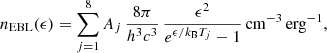
Relevant cosmic radiation fields include the CMB, a pure Planckian with a local temperature of TCMB = 2.735 K and energy density of uCMB = 0.25 eV cm−3, and the extragalactic background light (EBL). The latter originates from direct and dust-reprocessed starlight integrated over the star formation history the Universe, with two respective peaks that are referred to as the cosmic optical background (at ∼1 μm), and cosmic infrared background (at ∼100 μm). The two peaks are described as diluted Planckians, characterised by a temperature, T, and a dilution factor, Cdil. The latter is the ratio of the actual energy density, u, to the energy density of an undiluted blackbody at the same temperature, T (i.e., 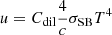 , where σSB is the Stefan–Boltzmann constant). The widely used EBL model, based on galaxy counts in several spectral bands (Franceschini & Rodighiero 2017), can be numerically approximated as a combination of diluted Planckians,
where Aj and Tj are suitable dilution factors and temperatures8.
Local radiation fields in the two galaxies (galactic foregound light, GFL) arise from their stellar populations. Similar to the EBL by shape and origin, the GFL is dominated by two thermal humps, IR and optical. Full-band luminosities of these thermal components are needed to determine n(ϵ), the spectral distributions of the photons to be Compton scattered (shown in Eq. (A.8)). We compute the total IR (8 − 1000 μm) luminosities using InfraRed Astronomical Satellite (IRAS) flux densities at 12 μm, 25 μm, 60 μm, and 100 μm (sampling the IR hump), from the relation fIR = 1.8 × 10⁻¹¹(13.48 f12 μm + 5.16 f25 μm + 2.58 f60 μm + f100 μm) erg cm−2 s−1 (Sanders & Mirabel 1996). The total optical luminosities are computed from narrow-band luminosities (H band for M31, B band for M33) by applying suitable bolometric corrections that restore the full-band luminosities. The corresponding energy densities, uk = Lk/[2πcRs(Rs+hs)], with k denoting either IR or optical, are:
(a) M31: The bolometric IR luminosity, LIR = 1.2 × 1043 erg s−1, is computed from the IRAS flux densities reported in Table 3. The bolometric optical luminosity, Lopt = 1.2 × 1045 erg s−1, is computed from the narrow-band 3.6 μm IRAC luminosity, LIRAC = 1.17 × 10¹¹ L⊙ (Courteau et al. 2011), multiplied by the bolometric correction, fbol = 2.7 (Rosenfield et al. 2012). Our region of interest is within R⋆ = 1.09 Rd, within which only 30% of the galaxy-wide emission is produced and is relevant to our GFL computation9. Given the relative thinness of the radio disk, only a negligible fraction of the radiation emitted at R > R⋆ enters the inner region. We obtain uIR = 0.04 eV cm−3 and uopt = 4 eV cm−3. The IR and optical hump temperatures reported in Table 3 imply dilution factors for the M31-sourced photon fields of cIR = 10−4.925, and Copt = 10−10.917;
M31 and M33: stellar-population emission parameters.
(b) M33: The bolometric IR luminosity, LIR = 4.8 × 1042 erg s−1, is computed from the data reported in Table 3. The total (bolometric) optical luminosity, Lopt = 3.1 × 1043 erg s−1, is computed from the de-reddened blue magnitude and color index,  and (B − V)0 ∼ 0.47 (Rice et al. 1988), by applying Buzzoni et al. (2006) bolometric correction as described in Persic & Rephaeli (2019a). Thus, uIR = 0.022 eV cm−3 and uopt = 0.14 eV cm−3. The IR and optical hump temperatures (Table 3) imply cIR = 10−5.267, and Copt = 10−12.436.
4. SED models
As mentioned, the main objective of this study is to determine the spectra of interstellar relativistic electrons and protons in the disks of M31 and M33 by a spectral modelling of the non-thermal emission in all the relevant energy ranges accessible to observations. In general, the particle, gas density, magnetic, and radiation field distributions vary significantly across galaxy disk, obviating the need for a spectro-spatial treatment: indeed, a detailed modelling approach based on a solution to the diffusion-advection equation has been applied in the study of the Galaxy and nearby galaxies where the spatial profiles of key quantities, such as the particle acceleration sources, gas density, magnetic field, and generally also the particle diffusion coefficient may be specified (e.g., Strong et al. 2007, 2010; Jones 1978; Taillet & Maurin 2003; Heesen 2021). However, if the aim is gaining insight on spatially-averaged non-thermal properties in the disk, then a parameter-intensive spectro-spatial modelling approach is not warranted. While ‘top-down’ diffusion-based modelling of the non-thermal emission in the disks and halos of galaxies is possible (Syrovatskii 1959; Wallace 1980; Rephaeli & Sadeh 2019), here we adopted a ‘bottom-up’ approach. Thus, we started from the non-thermal yields of relativistic particles and we deduced their steady-state spectra, making it is possible (in principle) to deduce the injection spectrum.
Radio emission in disks of spiral galaxies is mostly (electron) synchrotron in a disordered magnetic field whose mean total value, B, is taken to be spatially uniform in the regions of interest10 plus thermal free–free from a warm (∼104 K) ionised plasma (Spitzer 1978). This emission may be absorbed, at low frequencies, by cold (≲103 K) plasma (Israel & Mahoney 1980; Oster 1961)11. A significant proton component contributes additional radio emission by secondary e± produced by π± decays and γ-ray emission from π0 decay (Stecker 1971). In addition, γ-ray emission is produced by electron scattering off photons of local and background radiation fields (Blumenthal & Gould 1970). The calculations of the emissivities from all these processes are standard.
We just briefly expand here on thermal absorption of radio emission since it was not discussed in Paper I. A key feature in modelling the radio data is accounting for free–free absorption of non-thermal synchrotron by a warm thermal ionised plasma, as suggested by a high value of the Hα emission measure,  . This was originally pointed out for a sample of highly inclined spiral galaxies, including M33 and M31, based on the low ratio between the observed radio intensities and the intensities extrapolated from measurements at higher frequencies, with the ratio being smallest for edge-on galaxies (Israel & Mahoney 1980). The frequency-dependent optical depth for free–free absorption by thermal plasma is (Israel & Mahoney 1980):

whereby

where the electron temperature Te is in K, the frequency ν is in GHz, and the emission measure of the absorbing gas, EM, is in cm−6 pc−1. We assume that the radio emission and absorption are well mixed throughout the galaxy, so the emerging intensity is Iν ∝ jν(1 − e−τff(ν))/τff(ν), where jν is the (synchrotron plus thermal free–free) spectral emissivity and τff(ν) curves the spectrum at low frequencies.
We assume the particle spectral distributions to be time-independent and locally isotropic; then we have:
(a) The proton spectrum is:

for  (energies in GeV). The quantities Np, 0, qp are free parameters whose values will be determined by fitting the model to the data.
(b) Secondary electrons are produced from π± decays following p–p interactions of the protons with ambient gas: their spectrum has no free parameters once the proton spectrum is specified. A summary of secondary electron production is given in Appendix A.2.2. The secondary electron spectrum will be analytically approximated as
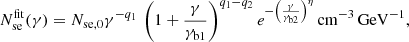
where q1, q2 and γb1, γb2 are the low- and high-energy spectral indices and breaks; and η gauges the steepness of the high-end cutoff. Their numerical values will be obtained by fitting Eq. (5) to the actual spectrum (Eq. (A.29)) which does not have any degrees of freedom. Thus, in our treatment, these are not free parameters.
(c) Primary electrons, required to fit the synchrotron data together with the secondary electrons, are chosen such that they approximate the steady-state electron spectrum following injection. Electron spectra are expressed as functions of the Lorentz factor, γ.
The emission spectrum from the π0-decay has more constraining power than a generic PL given its characteristic ‘shoulder’ at ≲100 MeV and its spectral cutoff corresponding to  . Thus, as in Paper I our modelling procedure begins with fitting a pionic emission profile to the γ-ray data with free normalisation, slope, and high-end cutoff. We then use the deduced (fully determined) secondary-electron spectrum together with a (modelled) primary electron spectrum to calculate the combined synchrotron emission using an independently estimated value of B. The fit to the radio data also includes, at high frequencies, a thermal bremsstrahlung component computed with literature-deduced values of the gas density and temperature, and thermal absorption at low frequencies. Finally, the full non-thermal bremsstrahlung and Comptonised-starlight γ-ray yields are determined using standard emissivities (see Appendix A) and added to the pionic yield to fit the γ-ray data. In principle, if the resulting model exceeds the LAT data, the proton spectrum is revised accordingly and the procedure is repeated until convergence: in practice, for M31 and M33, the leptonic γ-ray yields turn out to be quite small compared to the pionic yields, so no iteration is needed.
5. M31
In Ackermann et al. (2017), based on 7.3 yr of Fermi-LAT data, M31 was detected as extended with a significance of 4σ, with the favored model based on a disk of  radius. This result provides an estimate of the LAT sensitivity to source extension given the LAT instrumental response, the source spectrum, the diffuse backgrounds in the region, and the available statistics.
In Xing et al. (2023), based on 14 yr of LAT data, the measured emission was resolved into two regions, but now with a statistically significant evidence to reveal or rule out spatial extension. It is reasonable to assume that the γ-ray source associated with the M31 core has an extension (radius) of (at most)  – otherwise it would appear as extended in Xing et al. (2023), as found in Ackermann et al. (2017). In this subsection, we test the hypothesis of an extended γ-ray emission in the unresolved central region of M31, arising from truly diffuse LH emission and possibly an unresolved population of pulsars.
5.1. γ-ray yields
The average ambient proton density is np = nHI + 2 nH2 + ni ≃ 0.53 cm−3 (based on values listed in Table 4). A pionic fit, described by the parameters qp,  , up (reported in Table 5) matches the log-parabola best-fit from Xing et al. (2023) to the LAT data. In a fully pionic model, the unusually high value of up stems from the low hydrogen content in the central region of M31 (Fig. 12 of Nieten et al. 2006; the ‘central deficiency’ noted early on by, for instance, Davies & Gottesman 1970 and Emerson 1974): the proton energy-loss time by p–p interactions is
  , so for a given proton injection rate a low ambient gas density implies a high up.
M31 and M33: Interstellar medium parameters.
The closely related π±-decay secondary electron spectrum, Nse(γ), is computed as outlined above. Once the secondary synchrotron radiation has been computed (assuming B = 7.5 ± 1.5 μG; Fletcher et al. 2004, from particles-field equipartition), its low-frequency residuals from the radio data are modelled as synchrotron by a PL primary electron spectrum:

in the range of γmin < γ < γmax (with γmin ≫ 0), where the quantities Ne, 0, qe are free parameters. The ensuing primary and secondary leptonic γ-ray yields, namely, non-thermal bremsstrahlung and Comptonised starlight emission, are (at most) a few percent of the pionic emission. The LH γ-ray spectrum is plotted in Fig. 1 (top).
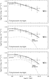 |
Fig. 1. γ-ray spectrum of emission from the central source of M31, |

The appropriate model for the LAT-measured γ-ray spectrum of M31 might be not just LH. The galaxy bulge and disk are characterised by a half-light radius of Re = 1 kpc and an exponential scale length of Rd = 5.3 kpc (Courteau et al. 2011), respectively. The upper limit to the central source radius, R⋆ = 5.45 kpc, includes the bulge and ∼30% of the (thin exponential) disk. So we may expect a γ-ray contribution from a fairly large unresolved population of γ-ray pulsars (PSR) located in the bulge and the inner disk12. The γ-ray PSR in M31 are expected to be similar to those in our Galaxy. The latter average spectral parameters are Γ = 1.6, Ecut = 2.5, and b = 1 (Abdo et al. 2013; Lopez et al. 2018). These values define a spectral shape inconsistent with the M31 LAT data. We incorporate the PSR spectrum and the LH spectrum into a mixed pulsar-plus-LH (PSR+LH) scenario. Possible examples of PSR+LH models involve Npsr = 500 (1000) PSR (Fig. 1, middle and bottom; and Table 5); since the M31 central source has L> 0.1 GeV = 1.4 × 1038 erg s−1 (Xing et al. 2023), PSR contribute 18% (36%) of the source luminosity in these models. Eyeball fits suggest that this family of PSR+LH models can nicely match the data for Npsr ≲ 1200 (and up ≳ 5 eV cm−3). If the unresolved PSR population is composed of msPSR, models using average Galactic msPSR γ-ray parameters, namely, L> 0.1 GeV = 3 × 1033 erg s−1, Γ = 1.3, Ecut = 2, and b = 1 (Abdo et al. 2013) can accommodate up to ∼104 msPSR.
M31 SED model parameters (within R⋆ = 5.45 kpc).
5.2. Radio yields
The radio emission measured in Battistelli et al. 2019 was integrated over the whole galaxy. To determine the primary electron densities in the region appropriate for calculating the γ-ray leptonic yields within R⋆, we need to estimate the radio flux from this region. To do so, we should know (in principle) the radial behavior of all the flux densities used in our analysis in order to build the radio SED integrated out to R⋆. From the literature, we took the radial profiles of the 408 and 842 MHz flux densities (Gräve et al. 1981, their Fig. 9). Both profiles are point-source-subtracted and averaged over circular rings centred on the nucleus of M31 and have a comparable overall appearance. As the 842 MHz profile appears to have a more regular, Gaussian-like shape (with a standard deviation of σ ≃ 1°), we assume that it is an adequate representative flux density profile. Integrating over a circular R⋆ region, we estimate that ∼15% of the total flux emanates from this region. Accordingly, our spectral fitting will be based on these reduced fluxes. Given the thinness of the disk, radiation produced in the outer disk is hardly captured by the < R⋆ region.
Reducing the flux according to the 842 MHz profile is a first-order correction to the galaxy-integrated flux. We expect flux-density radial profiles to steepen with increasing frequency because the corresponding higher-energy electrons diffuse out to shorter distances from their acceleration sites during their shorter energy loss time13. Moreover, the injection rate of freshly accelerated electrons is not sufficient to offset for their shorter radiative lifetimes because star formation rate declines fast with radius – even faster than the gas density (based on the Schmidt-Kennicutt law Σ ∝ σN with N > 1)14. The flux-density radial profiles at different frequencies have been measured in several nearby galaxies (e.g., M33: Tabatabaei et al. 2007; M51: Mulcahy et al. 2014) and a systematic (albeit usually moderate) radial steepening of the flux density profiles with increasing frequencies is clearly seen. We also expect this to be the case in M31 even though we are not aware of any available high-frequency data for this galaxy: if so, the emission fraction within R⋆ will be higher at GHz frequencies than the value we obtained at 842 MHz. So to compensate for the overcorrection inherent in the low-frequency-based first-order correction, which (as noted) is progressively more severe with increasing frequency, a second-order correction is needed. Lacking suitable spectral data, the strength of such second-order correction is uncertain: examples from M33 and M51 suggest a ≲25% increase at the highest frequencies. Thus, as the (unknown) second-order correction is probably small, we limited our correction to the first-order and calibrated the ≤R⋆ radio emission using the 842 MHz flux density profile. The main results of this paper will not be appreciably affected. For example, a 25% second-order correction can be compensated by a ∼40% increase in the thermal free–free emission leaving the non-thermal components essentially unchanged; alternatively, a flatter (qe = 3) and lower (by a factor of ∼4) electron spectrum would leave the pionic component virtually unaffected.
We wish to reproduce the M31 radio spectral model presented by Battistelli et al. (2019) self-consistently in the context of our approach. Synchrotron emission by secondary electrons (no degrees of freedom) dominates the radio emission up to ∼2 GHz. Fitting to the synchrotron by primary electrons results in a spectral index, αr ≃ 1.1, matching the total synchrotron fitting value of  from Battistelli et al. (2019). With no evidence of a spectral cutoff in the data, we set the primary electron maximum energy at γmax = 6 × 10⁴. The synchrotron spectrum from Battistelli et al. (2019) turns over at ν ∼ 48 MHz; as we do for M33 (Sect. 4.2.2), we interpret this feature as absorption by a cold plasma cospatial and homogeneously mixed with the electrons (Spitzer 1978); this is a common feature in highly inclined disk galaxies (Israel & Mahoney 1980). M31’s perpendicular emission measure EM0 ∼ 30 cm−6 pc−1 (Walterbos & Braun 1994) implies, for a galaxy inclination of 77°, a line-of-sight value of EM = EM0/cos(77° ) = 133 cm−6 pc−1. Assuming a temperature
  = 550 K for the cold plasma (similar to M33, see Sect. 4.2.2), from Eqs. (2) and (3), we can derive an optical depth, which matches the model from Battistelli et al. (2019) at ν < 100 MHz. A ν−0.1 component in the Battistelli et al. (2019) model accounts for a slight spectral concavity at ν > 1 GHz. We modelled it as thermal free–free emission in the parametrisation reported in Eq. (A.12), which gauges this flux with the Hα flux assuming that both emissions come from the same emitting (HII) regions with the same plasma parameters (temperature, density, filling factor), so the measured Hα flux may be used to predict the free–free emission. The radio spectrum is shown in Fig. 2, overlaid with the Battistelli et al. (2019) fit (top) and our model (bottom).
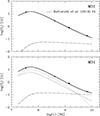 |
Fig. 2. Radio spectrum of M31. The data points (from Battistelli et al. 2019) denote the whole-galaxy radio flux reduced to the estimated flux expected from within the R⋆ radial region as described in the text. Also shown are: (top) Battistelli et al. (2019) fit (single electron population synchrotron: dotted curve; thermal free–free emission: dot-dashed curve), and (bottom) our LH emission model. The latter includes primary and secondary synchrotron radiation (dotted curves of increasing flux at their peaks) and a thermal free–free component (dot-dashed curve). |
5.3. Broadband results and discussion
The broadband SED models of the M31 central source are shown in Fig. 3. The fitting parameters are given in Table 5.
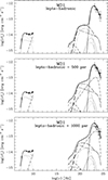 |
Fig. 3. Broadband lepto-hadronic SED of the M31 central source: data points are shown as dots (with errorbars indicating frequency and flux uncertainties), model predictions as curves (top). The galaxy-wide flux densities of Battistelli et al. (2019) have been renormalised to the region encompassed by R⋆ (i.e., ∼15% of the total emission; see Sect. 4.1.2). Emission components are denoted by these line types: radio synchrotron, dotted; thermal free–free emission, dot-dashed; total radio, solid; Comptonised CMB, short-dashed; Comptonised starlight (EBL+FGL), long-dashed; non-thermal bremsstrahlung, dotted; pionic, solid. Leptonic emission includes that from primary and secondary electrons(secondary components are dominant). In the X-ray/γ-ray range, on top of the separate components, a thick solid line indicates the total emission. Same for a broadband PSR+LH SED (middle). The 500 pulsars emission component (see text) is ahown as a dot-dashed line. Same as above but for 1000 pulsars (bottom). Note: in this case the secondary leptonic components are subdominant. |
The small statistics of the available γ-ray data (five LAT spectral points) do not allow for a clear statement about the pulsar contribution, which however appears to marginally improve the fit at ∼2 GeV. Indeed, a consistent population of γ-ray pulsars is very likely to exist in M31: in the (“twin”) Milky Way galaxy, about 300 pulsars have been detected by Fermi-LAT as of August 202315 and thousands of unresolved msPSR have been proposed as candidates to interpret the Galactic Center “GeV excess” (Brandt & Kocsis 2015; Bartels et al. 2016; Arca-Sedda et al. 2018; Fragione et al. 2018a,b; Miller & Zhao 2023; Malyshev 2024; for a different view see Crocker et al. 2022).
The values of up obtained from the SED modelling are much higher than the local Galaxy value of 1 eV cm−3 (e.g., Webber 1987). An independent estimate (see Sect. 5) suggests up ∼ 5 cm−3 for the average proton energy density within R⋆. If so, the PSR+LH model with 1000 PSR may be more realistic.
We note a similarity between the values of the proton spectral index in M31, deduced from our SED modelling, and in the Milky Way, from the measured cosmic-ray flux at the Sun position (e.g., Gaisser 1990). The local Galactic value, qp = 2.7, is understood as resulting from injection and diffusion, qp = qinj + δ with qinj ∼ 2.2 (typical of supernova remnants like the Crab Nebula) and δ ∼ 0.5 (e.g., Ptuskin 2006).
Any current view on the nature of the central engine may change if the Fermi-LAT spatial resolution may improve, for instance, as a consequence of a long future operating lifetime. The central source could either be resolved into multiple sources or confirmed to be pointlike at the centre. As to the latter possibility, in the next paragraph, we briefly discuss the possibility that the pointlike source at the centre is identified with M31’s nuclear supermassive black hole (BH), M31*.
A comparison with Sagittarius A* (Sgr A*, the supermassive BH at the Galactic Centre) may be useful. Cafardo & Nemmen (2021) found that the centroid of the 0.1–500 GeV emission, measured by Fermi-LAT (∼11 yr of data), approaches Sgr A* as the energy increases (at 10 GeV the two positions coincide within 1σ): at the Galactic Center distance, Cafardo & Nemmen (2021) point-like source has L0.1 − 500 GeV = 2.6 × 1036 erg s−1, a value consistent with the Sgr A* bolometric luminosity. The mass of M31* is 7.5 × 10⁷ M⊙ (Ford et al. 1994), whereas that of Sgr A* is 4.3 × 10⁶ M⊙ (Ghez et al. 2008). As for the X-ray luminosities, that of M31* is 2 × 1036 erg s−1 (Garcia et al. 2010; Li et al. 2009), whereas that of Sgr A* fluctuates between ∼1033 (baseline) and ∼1035 during the hr-timescale daily flares (Sabha et al. 2010). Thus, both M31 A* and Sgr A* emit at level ≲10−10LEdd, with LEdd = 1.26 × 1038 (M/M⊙) erg s−1 the Eddington luminosity. This suggests that both M31* and Sgr* are currently dormant supermassive BHs. Therefore, if the pointlike source identified by Cafardo & Nemmen (2021) at the Galactic Centre is the γ-ray counterpart of Sgr A*, with the γ rays produced by relativistic particles accelerated by (or in proximity of) the BH (Cafardo & Nemmen 2021; Ajello et al. 2021) and if a scaling relation of yet unspecified nature (Aharonian & Neronov 2005) exists between the γ-ray luminosity and the BH mass, then for the γ-ray counterpart of M31* we may expect L0.1 − 500 GeV = 5 × 1037 erg s−1; this value that corresponds to ∼1/2 of the luminosity of the central source identified by Xing et al. (2023). In this case, the pointlike central source in M31 may be related to M31*. A study of the flux variability (tvar = Rs/c = 104 MBH/(109 M⊙) s) may clarify the issue. Lacking a clear prediction on the γ-ray spectral signature from a supermassive BH, we generally expected the γ-ray emission of M31* to be partly pionic, from relativistic protons accelerated near the BH (perhaps by winds; see Ajello et al. 2021; Kimura et al. 2021) and interacting with the inflowing gas, and partly leptonic from the Comptonisation of the optical/X-ray radiation in the immediate proximity of the BH (coming from, e.g., the accretion disk; Dermer et al. 1992). If so, the BH γ-ray emission may be similar in spectral shape to the diffuse pionic emission tracing the (low-density) hydrogen distribution within R⋆. These two emission components would not be separated based on current LAT data, and the high proton (and ensuing secondary electron) density derived from the purely pionic fit may be an artifact due to spectral confusion.
5.4. Summary on M31
The broadband radio–γ-ray non-thermal emission of M31 studied in this paper originates in the central (R ≤ R⋆ ≃ 5.5 kpc) region. This radial scale is dictated by the Fermi-LAT sensitivity to source extension within which unresolved (i.e., point-like) emission has been detected by Xing et al. (2023). The radio (synchrotron and thermal free–free) emission from this region has been estimated starting from the all-disk integrated emission, using the radial profile of the 842 MHz emission line.
We suggest that the emission from M31’s central region can be spectrally modelled as diffuse pionic with likely contributions from an unresolved population of ∼1000 Galactic-like pulsars plus the nuclear BH (M31*). In fact, the central ‘hydrogen hole’ may allow for emission from the enclosed pulsar population and M31* to pass through. While the Galactic-like-pulsar emission used in our model differs in spectral shape from the pionic emission, the (putative) BH emission may be quite similar to it hence the two would not be separated based on current data. Thus, the proton component of the non-thermal interstellar gas, derived from a purely diffuse pionic fit to current LAT data, would be biased towards high values due to contamination from M31* emission.
6. M33
Based on 11.4 yr of LAT data, Xi et al. (2020) detected a statistically significant emission from M33. Although it peaks on the northeast region of the galaxy, where the giant HII region NGC 60416 is located, the LAT signal appears to originate from the whole galaxy. This is suggested by the fact that spatially extended templates based on IR maps of M33 (IRAS at 60 μm, and Herschel Photoconductor Array Camera and Spectrometer [PACS] at 160 μm) give almost equally good fits as the point-source model centred at the (NGC 604-related) best-fit location (Xi et al. 2020). The morphological correlation between IR and γ-ray emission suggests the latter to be of mainly pionic origin.
6.1. Pionic yields
The ambient proton density is np ≃ 1.92 cm−3 (see Table 4 for densities in the different phases of the interstellar gas). The parameters describing the proton spectrum that matches the LAT data are listed in Table 6; in particular, the PL slope agrees with the values reported by Xi et al. (2020) for the nominal 0.1–80 GeV LAT spectrum (Fig. 4). The respective relativistic proton energy density is up = 0.46 eV cm−3.
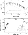 |
Fig. 4. SED of M33. Radio spectrum (top): the emission model (solid curve), including primary and secondary synchrotron radiation (dotted curves of decreasing flux) as well as a thermal free–free component (dot-dashed curve), is overlaid with data from Table 2 (black dots). The empty squares represent the estimated radio flux after removing the contribution from ≤200 pc size sources (Tabatabaei et al. 2022). The total radio emission, resulting if the ‘nominal’ primary electron spectrum is used, is indicated by the dashed curve. Broadband SED (bottom): data points are shown as dots, model predictions as curves. Emission components are plotted by the following line types: radio synchrotron, dotted; thermal free–free emission, dot-dashed; total radio, solid; Comptonised CMB, long-dashed; Comptonised starlight (EBL+FGL), short-dashed; non-thermal bremsstrahlung, dotted; and pionic, solid. For each type of non-thermal leptonic yield, the total, primary, and secondary emissions are denoted as curves of progressively lower flux. In the X-ray and γ-ray range, on top of the separate components, a solid line indicates the total emission. The empty squares and dashed curve in the radio are as described in the top panel. |
M33 SED model parameters (galaxy-wide).
The closely related π±-decay secondary electron spectrum, Nse(γ), is computed as described in Sect. 4. The parameters of its analytical fitting function, Nse(γ), are given in Table 6. The corresponding synchrotron emissivity is specified in Eq. (A.6).
6.2. Leptonic yields
To compute the electrons synchrotron emission we assume the relevant average total magnetic field in which primary and secondary electrons are immersed to be B = 6.5 μG (Tabatabaei et al. 2008). Once the secondary electron synchrotron yield has been computed, its low-frequency residuals from the data are modelled by attributing them to primary electrons.
To find the spectrum of the primary electrons, we adopt a phenomenological approach. We first try a PL spectrum but its resulting synchrotron emission (see Eq. (A.4)) grossly misses the data. We then use a smooth double-PL (2PL) spectrum:

where Ne0 is the normalisation, α and β are the low/high-energy slopes, γb is the break energy, and γmax is the cutoff energy. Comparison with the steady-state electron spectrum in the presence of radiative losses (see Sect. 4) suggests that α = qinj − 1 and β = qinj + 1, where qinj is the injection spectral index. So the adopted 2PL spectrum is finally written as

where Ne0, qinj, γb are free parameters. The corresponding synchrotron emissivity is specified in Eq. (A.5).
The high measured value of the Hα emission measure (Deharveng & Pellet 1970) and the sub-GHz turnover of the radio spectrum (Israel et al. 1992) suggest free–free absorption of the radio emission at low frequencies by a cool ionised plasma. The Galactic-absorption corrected EM in the direction to the observer (galaxy inclination is i = 57°) is EM = 64 cm−6 pc−1 (Monnet 1971). By definition, the EM is an integral quantity, so a detailed knowledge of the diffuse ionised gas along the line of sight is not needed. In agreement with (Israel et al. 1992), we find that, independent of the electron injection index, absorption of the non-thermal emission by a Te ∼ 500 K plasma is required to fit the ≲100 MHz data.
At high frequencies, the ν−0.1 component represents diffuse thermal free–free emission. This emission may be gauged to the Hα flux if both come from the same HII regions since in this case the relevant warm-plasma parameters (temperature, density, filling factor) are the same: In this case, the measured Hα flux may be used to predict the free–free emission. Following the latter approach (Klein et al. 2018), we modelled the thermal free–free emission from Eq. (A.12) using  for the warm plasma and F(Hα) = 2 × 10⁻¹⁰ erg cm−2 s−1 (only 40% of the integrated Hα flux, 5 × 10⁻¹⁰ erg cm−2 s−1, is diffuse: Verley et al. 2009; also Hoopes & Walterboos 2000)17. The radio measurements and model, which includes primary and secondary synchrotron and thermal emission, are shown in Fig. 4 (top).
With the electron spectra determined, we can calculate the Compton and non-thermal-bremsstrahlung yields from electrons scattering off, respectively, CMB-EBL-GFL photons and thermal plasma nuclei using Eqs. (A.7)–(A.8). Although the shape of the γ-ray spectrum is distinctly pionic, the Comptonised starlight peaks near the pionic peak (ν ∼ 2 × 10²³ Hz), where it contributes 5% of the measured flux, and the non-thermal-bremsstrahlung peaks at ν ∼ 3 × 10²³ Hz, where it contributes 1%.
6.3. Results and discussion
While comparison of the LH SED model to the dataset is not formally a best-fit, the agreement is reasonable, given the independently set priors on the values of B and q1, and two of its features are well based. The first is the pionic fit to the LAT data: the γ-ray leptonic contribution is very minor, even with the appreciable level of he uncertainty in the electron spectral parameters (see below). The LAT data, however, show no spectral cutoff; the central value of the last LAT datapoint implies  GeV, and even with the uncertainty reflected in the width of the energy band, it is still clear that
  GeV.
GeV.
The second apparent feature is absorption of the synchrotron emission by warm thermal gas. It is clear that even for the hardest possible primary electron spectrum (qinj = 2) and in spite of the substantial scatter of data, the spectrum at ≤100 MHz can only be reproduced with absorption by a low-temperature (500 K) thermal gas, in accordance with a suggestion made by Israel et al. (1992), and similarly (for NGC 891) by Mulcahy et al. (2018).
The relatively flat γ-ray slope of M33 suggests that, unlike for M31, a substantial PSR contribution is unlikely. The PSR spectral cutoff (at several GeV) results in a spectral hump in the relevant energy range (see Fig. 1). This in contrast to the relatively flat PL-like pionic model that appears to naturally match the data.
The uncertainty in the total (HI, H2, HII) gas density affects the energy-loss coefficients used to compute the secondary electron spectrum (Paper I) and the ensuing normalisation and shape of the primary electron spectra and their yields. However, the electron density is effectively unconstrained because it depends on assuming a magnetic field value rather than using a value derived by modelling the non-thermal–X-ray emission as Comptonised CMB (e.g., Persic & Rephaeli 2019a,b) or the hard X-ray–MeV as Comptonised infrared (IR) radiation.
A further source of uncertainty in modelling the primary electron spectrum comes from the large scatter in the radio data. A strong coupling among Ne0, qinj, γb implies a broad range of acceptable values of these parameters (Table 4) because a non-linear combination of qinj and γb determines the effective synchrotron slope at ≳1 GHz which, for an assumed B (derived assuming equipartition between the energy densities of the magnetic field and relativistic particles; Tabatabaei et al. 2008), determines the primary electron normalisation Ne0. That said, we may surmise qinj = 2.25 is realistic for M33 based on the following argument. Electron indices measured in Galactic supernova remnants peak at 2.15 ≤ qe ≤ 2.3 (Mandelartz & Becker 2015), and values in the same range are also found in the quietly star-forming Magellanic Clouds (Paper I). As for the proton indices, which closely reflect the injection index given the low energy losses suffered by protons via p–p interactions with the local medium, values in a similar range are found, 2.2 ≤ qp ≤ 2.6 (Mandelartz & Becker 2015; Paper I). Thus, a value qinj = 2.25 is quite reasonable for both protons and electrons. The corresponding energy density ratio between proton and (primary) electron, ≃22, is higher than its value for PL injection spectra, ≃17 (Persic & Rephaeli 2014), as a consequence of the higher energy losses of electrons than of protons. Finally, the electron cutoff energy γmax is constrained low enough as not to overproduce the flux at ≥2700 GHz and high enough not to violate the highest-frequency point (interpreted as an upper limit by Israel et al. 1992).
The data from Israel et al. (1992), while free from the major individual sources that could have been identified when the observations were made, are not free from the integrated source emission of fainter sources. Tabatabaei et al. (2022) pointed out that radio sources with sizes ≤200 pc constitute ∼36% (46%) of the total radio emission at 1.5 (6.3) GHz in the inner 4 kpc × 4 kpc disk of M33. Indeed, the nominal steady-state primary electron spectrum, Npe(γ) = kinj/(qinj − 1) γ−(qinj − 1)/(b0 + b1γ + b2γ2), where  is the electron spectral injection rate and the bj terms denote Coulomb, bremsstrahlung, and synchrotron and Compton energy losses, as in Eqs. (A.23)–(A.25), while neglecting diffusion and advection losses. While it ends up under-reproducing the Israel et al. (1992) data, it is still compatible with the suggestion from Tabatabaei et al. (2022). If so, the X-ray and γ-ray leptonic yields would be even lower, making the LAT-measured emission even more likely to be of pionic origin.
Less noisy radio data are needed to clarify several issues. At low frequencies more precise ≲100 MHz data would help to constrain the cold-plasma temperature in the range of  . This is essential because a more accurate determination of
  is key to our knowledge of the cold gas in galactic halos (which are best studied in inclined galaxies by measuring the absorption of radio emission from their disks; e.g., Dettmar 1992). For example, in the framework of the present analysis, the high-resolution 74 MHz VLSS18 data (Cohen et al. 2007) may be suitable to this aim after integrating the M33 map over the whole disk and suitably subtracting point sources in order to achieve consistency with the data in Israel et al. (1992). At higher frequencies, the data between 100 MHz and 2 GHz, which is free from plasma absorption and located in the bremsstrahlung energy-loss regime19, where the electron spectrum is Ne(γ)∝γ−qinj, would constrain qinj and thereby allow for a more reliable determination of the primary electron spectrum.
7. Conclusion
In this paper, we present a spectral fitting of electron and proton radiative yields to radio and γ-ray measurements of the Local Group galaxies M31 and M33, namely: the central region (≲5.5 kpc) for M31 and the whole disk for M33. For M31, our analysis suggests that a combination of diffuse pionic, pulsar, and nuclear-BH–related emissions could explain the LAT data. For M33, our analysis clearly indicates that the LAT-measured emission is mostly of pionic origin in agreement with Xi et al. (2020). While uncertainties in the 3D galaxy structure directly affect the overall normalisations of the particles spectral distribution functions, the model SEDs are essentially unaffected by variations of the galaxy structure parameters.
Future measurement of diffuse non-thermal X-ray emission from the galactic disks will substantially improve the SED fits and result in improved determinations of the particle spectral parameters. For example, measurements of non-thermal 1 keV flux that result (mostly) from Compton scattering of the electrons by the CMB fix the overall normalisation of the electron spectrum (Persic & Rephaeli 2019a,b). This follows from the fact that the good pionic fit to the γ-ray emission firmly determines the secondary electrum spectrum, which then effectively leads to the primary electron normalisation, Ne0. Modelling the radio spectrum as synchrotron would then provide the (volume-averaged) magnetic field, B. A spectral determination of B would remove the need to assume particle-field equipartition or to use line-averaged fields, such as those derived by Faraday rotation studies of extragalactic polarised sources seen through the disk.
Given the importance of magnetic fields in modelling non-thermal SEDs, a comment on the values we have adopted in this study is in order. Mean values of the magnetic fields of both galaxies adopted from radio studies of M31 (Fletcher et al. 2004) and M33 (Tabatabaei et al. 2008) rely on the assumption of energy density equipartition between relativistic particles and magnetic field. In estimating relativistic electron and proton densities from radio measurements, the electron densities can be readily derived but assumptions must be made on the associated proton number (energy) densities that are also required to estimate the equipartition magnetic field, Beq. Fletcher et al. (2004) used up/ue = 100 in the standard equipartition formula, Beq ∝ (1 + up/ue)2/(5 + qe) (e.g., Persic & Rephaeli 2014), whereas Tabatabaei et al. (2008) used Np/Ne = 100 in the ‘modified’ equipartition formula: Beq ∝ (1 + Np/Ne)2/(5 + qe) (Beck & Krause 2005). Our SED model for M31 exhibits up/ue ∼ 100, in agreement with Fletcher et al. (2004). As for M33, the quantity Np/Ne can be estimated as follows. Assuming radiative losses only, particle number densities are nearly constant (when integrated over energy) over time, thus, the particle number ratio can be calculated at injection: for an electrically neutral non-thermal plasma: Np/Ne = (mp/me)(qinj − 1)/2 (Schlickeiser 2002). Our M33 SED model has qinj = 2.25 (Table 6), so Np/Ne = 110. This numerical coincidences suggest that equipartition between relativistic particles and magnetic field (i.e., minimum energy in the non-thermal fluid; Longair 1981; Govoni & Feretti 2004), is achieved in the central region of M31 and the disk of M33; these serve as a posteriori proof that our models use the B-values from Fletcher et al. (2004) and Tabatabaei et al. (2008) in a self-consistent way. Finally we note that because Beq ∝ (1 + ρp/ρe)2/(5 + qe)≃0.27, where ρj denote energy (number) density for M31 (M33), the derived equipartition fields are relatively stable against variations of these quantities.
Concerning the magnetic field in M31, we should note that the approximately constant field B ≃ 7.5 μG derived by Fletcher et al. (2004) spans galactocentric radii of 6 kpc < R < 14 kpc. In the present analysis, we extrapolated that value inwards into the region R < R⋆ = 5.5 kpc relevant to our study. The justification to do so on the fact that the average plasma density measured out to R ∼ 10 kpc is ni ∼ 0.05 (Trudoljubov et al. 2005), based on modelling the interaction between supernova remnants and the diffuse hot ionised plasma with a non-equilibrium collisional ionisation model. This value is close to that reported in Table 4 for the central region R ≤ 5.5 kpc. Since ne = Z2ni, the scaling relation  (Rephaeli 1988) substantiates our decision to extrapolate the Fletcher et al. (2004)B-value into the central region of M31.
An independent estimate of up may provide a consistency check of the preferred (mostly) hadronic models of the γ-ray data of M31 and M33. Combining the SN frequency with the residency timescale, which represents the characteristic proton residence time in the disk, τres, (and assuming a nominal value of the fraction of total SN energy that is channeled to particle acceleration) enables an estimation for up (e.g., Persic & Rephaeli 2010). Assuming no appreciable mechanical energy loss (e.g., in driving a galactic wind), the value of τres is determined by the energy-loss timescale for p–p interactions, τpp = (σppcnp)−1. At the most relevant energy range (σpp ≃ 40 mb), the characteristic value is  yr. During τres, a number νSNτres of SN explode in a region of volume, V, thus depositing the kinetic energy of their ejecta, Eej = 1051 erg per SN (Woosley & Weaver 1995), into the interstellar medium. Arguments based on the cosmic-ray energy budget in the Galaxy and SN statistics indicate that a fraction η ∼ 0.05 − 0.1 of this energy is available for accelerating particles (e.g., Higdon et al. 1998; Tatischeff 2008). Accordingly, we express the proton energy density as:
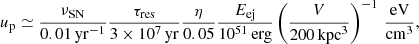
where the various quantities are normalised to typical Galactic values. The results are as follows:
(a) In the M31 disk region, we are considering (R ≤ R⋆ = 5.45 kpc), the average gas density is ng ≃ 0.5 cm−3 hence τres ∼ τpp = 6 × 10⁷ yr. The galaxy-wide SN rate is νSN ≃ 0.01 yr−1 (type Ia: 0.006 ± 0.004, van den Bergh 1988; type II: 0.004, from Eq. (14) of Persic & Rephaeli 2010 using LIR). Assuming the local SN rate to scale as the stellar surface brightness, the SN rate integrated within R⋆ (corresponding to 1.09 Rd) is 0.3 νSN. Then, Eq. (9) yields up ≃ 7 eV cm−3, which is compatible with the value suggested by our PSR+LH model with 103 PSR. We note that a similar value, ∼6 eV cm−3, was deduced for the inner Galactic plane from γ-ray observations (Aharonian et al. 2006).
(b) In M33, the galaxy-wide average gas density is np ∼ 2 cm−3; hence, τres ∼ τpp ∼ 107 yr. The total (mostly core-collapse, type II) SN rate is νSN ≃ 0.003 yr−1 (van den Bergh & Tammann 1991; Pavlidou & Fields 2001). Then, Eq. (9) yields up ≃ 0.6 eV cm−3 (galaxy average), in fair agreement with the SED modelling result20.
We conclude with a remark on the detectability of the p–p related neutrino emission via π± decay from M31 and M33. With the proton spectrum fully determined by our fit to the measured γ-ray emission, we estimated (using Kelner et al. 2006 formalism, reported in Appendix A.2.3) that the broadly peaked (∼0.1–10 GeV) π±-decay neutrino fluxes from the two galaxies are ∼60 (M31) and ∼100 (M33) times lower than the flux from the Large Magellanic Cloud reported in Paper I. These fluxes are too low to make detections using any of the current and upcoming neutrino projects.
For our purposes, the source regions of the two galaxies are modelled as cylinders of radius and height Rs = 5.45 kpc and hs = 0.24 kpc (Brinks & Burton 1984) for M31, and Rs = 8.7 kpc and hs = 0.2 kpc (Kam et al. 2015; Monnet 1971) for M33.

86 sources in the central ∼34′ down to L0.2 − 4 keV = 1.4 × 1036 erg s−1 from a 48 ks observation with the High Resolution Imager (HRI; Primini et al. 1993); and 396 sources within 6.3 deg2 in the luminosity range to 3 × 1035 < L0.1−2.4 keV/erg s−1 < 2 × 1038 from a 205 ks observation with the Position Sensitive Proportional Counters (PSPC; Supper et al. 1997), respectively.
Hard (3−100 keV) X-ray data the emission shows two components, one broadly peaking at ∼5 keV, and another extending to > 100 keV, that are interpreted as arising from NS binaries with, respectively, high/low accretion rates and luminosities above/below ∼1037 erg s−1 (Revnitsev et al. 2014: Rossi X-ray Timing Explorer (RXTE)/Proportional Counter Array (PCA), INTErnational Gamma-Ray Astrophysics Laboratory (INTEGRAL)/Integral Soft Gamma-Ray Imager (ISGRI), and Neil Gehrels Swift Observatory/Burst Alert Telescope (BAT) data).
Based on 33 months of High Altitude Water Cherenkov (HAWC) telescope data, an upper limit was set on the 1−100 TeV flux from the galactic disk of M31 (Albert et al. 2020).
The optical size of M33, as measured by the 25-mag-arsec−2 radius, is R25 = 35.4′; De Vaucouleurs et al. (1991).
Combining all ROSAT observations Haberl & Pietsch (2001) conclusively found 184 sources within 50″ of the nucleus.
The bulge contribution is very minor (Soifer et al. 1986).
This assumption is realistic for the two galaxies considered in this paper (M31: Table 1 of Fletcher et al. 2004; M33: Fig. 9 of Tabatabaei et al. 2008) and it also appears to be valid overall (Beck 2016).
For a review on the multiphase insterstellar medium, see Cox (2005).
If the LAT data need to be modelled as pure pulsar emission, a decent match is obtained for Npsr = 3500 Galactic-like pulsars emitting, through a photon spectrum dN/dE ∝ E−Γe−(E/Ecut)b (Abdo et al. 2013), where Γ = 2, Ecut = 3 GeV, and b = 0.6 at a luminosity level L> 0.1 GeV = 5 × 1034 erg s−1.
The diffusion length is  where D is the (constant) diffusion coefficient and τ is the particle radiative lifetime. For synchrotron losses it is τ = γ/bsyn ∝ γ−1 (where bsyn ∝ γ2 is the synchrotron loss term, see Eq. (A.27)), hence, ℒD ∝ γ−1/2.
Σ and σ are surface densities of, respectively, star formation rate and gas. The exact value of N depends on the gas tracer (HI or H2 or their sum) and the particular galaxy (e.g., DeGioia-Eastwood et al. 1984 for NGC 6946, and Elia et al. 2022 for the Milky Way; see also reviews by Kennicutt 1998; Kennicutt & Evans 2012).
NGC 604 is a very active star-forming region that, within a cavity near the centre of the nebula, contains > 200 massive blue stars – some with masses exceeding 120 M⊙ and surface temperatures of ∼7 × 10⁴ K. The cavity itself is blown by the collective stellar winds from these stars, whose strong ultraviolet radiation makes the surrounding gas fluorescent.
For consistency we note that computing the free–free emissivity using Z2ni = ne = 0.03 cm−3 (derived from the Hα emission measure; Tabatabaei et al. 2008) for the warm plasma in Eq. (A.9) we obtain a spectral flux consistent with the one derived from the integral Hα flux in Eq. (A.11).
For the assumed B = 6.5 μG (Tabatabaei et al. 2008) the characteristic synchrotron frequency, νs = 3γ2B MHz implies a range of electron energies 2.3 × 10³ ≲ γ ≲ 104 emitting between 100 MHz and 1 GHz. This range is well inside the bremsstrahlung-loss–dominated regime, 600 ≤ γ ≤ 25 000.
The agreement between the values of up given by Eq. (9) and those returned by the SED modelling also holds for the Magellanic Clouds studied in Paper I:
(a) Large Magellanic Cloud: r = 3.5 kpc, h = 0.4 kpc, np = 0.6 cm−3, νSN = 10−3 yr−1 (Chu & Kennicutt 1988) → up = 1.3 eV cm−3, versus  eV cm−3; and
(b) Small Magellanic Cloud: r = 1.6 kpc, h = 4 kpc, np = 0.6 cm−3, νSN = 6.5 × 10⁻⁴ yr−1 (Kennicutt & Hodge 1986) → up = 0.6 eV cm−3, versus  eV cm−3.
For illustration purposes, we set σpp = σpp, 0. (It is σpp, 0 ≃ 30 mbarn for 5 ≲ Ep/GeV ≲ 50.) The corresponding injection spectrum, Qse(γ) = (8/3) me (c/kπ±) np σpp, 0 Np0 [mp+(4me/κπ±) γ]−qp cm−3 s−1 (unit of γ)−1 valid for γ > γthr, coincides with the exact solution except for a monotonic, rather than curved, spectral shape in the range γthr < γ ≲ 150.
Acknowledgments
We acknowledge constructive comments by an anonymous referee. M.P. thanks the Physics and Astronomy Department of Padova University for hospitality.
References
- Aaij, R., Adeva, B., Adinolfi, M., et al. 2015, JHEP, 1502, 129 [CrossRef] [Google Scholar]
- Abdo, A. A., Ackermann, M., Ajello, M., et al. 2010, A&A, 523, L2 [CrossRef] [EDP Sciences] [Google Scholar]
- Abdo, A. A., Ajello, M., Allafort, A., et al. 2013, ApJS, 208, 17 [Google Scholar]
- Achilli, A., Srivastava, Y., Godbole, R., et al. 2011, Phys. Rev. D, 84, 094009 [NASA ADS] [CrossRef] [Google Scholar]
- Ackermann, M., Ajello, M., Allafort, A., et al. 2012, ApJ, 755, 164 [NASA ADS] [CrossRef] [Google Scholar]
- Ackermann, M., Ajello, M., Albert, A., et al. 2017, ApJ, 836, 208 [CrossRef] [Google Scholar]
- Aharonian, F. A., & Atoyan, A. M. 2000, A&A, 362, 937 [NASA ADS] [Google Scholar]
- Aharonian, F., & Neronov, A. 2005, ApJ, 619, 306 [CrossRef] [Google Scholar]
- Aharonian, F., Akhperjanian, A. G., Bazer-Bachi, A. R., et al. 2006, Nature, 439, 695 [Google Scholar]
- Ajello, M., Baldini, L., Ballet, J., et al. 2021, ApJ, 921, 144 [CrossRef] [Google Scholar]
- Albert, A., Alfaro, L., Alvarez, C., et al. 2020, ApJ, 893, 16 [NASA ADS] [CrossRef] [Google Scholar]
- Arca-Sedda, M., Kocsis, B., & Brandt, T. 2018, MNRAS, 479, 900 [NASA ADS] [CrossRef] [Google Scholar]
- Baars, J. W. M., Genzel, R., Pauliny-Toth, I. I. K., & Witzel, A. 1977, A&A, 61, 99 [NASA ADS] [Google Scholar]
- Bartels, R., Krishnamurthy, S., & Weniger, Ch. 2016, Phys. Rev. Lett., 116, 051102 [CrossRef] [PubMed] [Google Scholar]
- Battistelli, E. S., Fatigoni, S., Murgia, M., et al. 2019, ApJ, 877, L31 [Google Scholar]
- Beck, R. 2000, in The Interstellar Medium in M31 and M33, eds. E. M. Berkhuijsen, R. Beck, & R. A. M. Walterbos (Aachen: Shaker), 171 [Google Scholar]
- Beck, R. 2016, A&A Rev., 24, 4 [NASA ADS] [CrossRef] [Google Scholar]
- Beck, R., & Krause, M. 2005, Astron. Nachr., 326, 414 [Google Scholar]
- Berkhuijsen, E. M., Beck, R., & Hoernes, P. 2003, A&A, 398, 937 [NASA ADS] [CrossRef] [EDP Sciences] [Google Scholar]
- Blumenthal, G. R., & Gould, R. J. 1970, Rev. Mod. Phys., 42, 237 [Google Scholar]
- Bogdan, A., & Gilfanov, M. 2008, MNRAS, 388, 56 [NASA ADS] [CrossRef] [Google Scholar]
- Braccesi, A., Fanti-Giovannini, C., Fanti, R., et al. 1967, Nuovo Cimento, B52, 254 [Google Scholar]
- Brandt, T. D., & Kocsis, B. 2015, ApJ, 812, 15 [Google Scholar]
- Brinks, E., & Burton, W. B. 1984, A&A, 141, 195 [NASA ADS] [Google Scholar]
- Buczilowski, U. R. 1988, A&A, 205, 29 [NASA ADS] [Google Scholar]
- Buzzoni, A., Arnaboldi, M., & Corradi, R. L. M. 2006, MNRAS, 368, 877 [Google Scholar]
- Cafardo, F., & Nemmen, R. 2021, ApJ, 918, 30 [NASA ADS] [CrossRef] [Google Scholar]
- Chu, Y.-H., & Kennicutt, R. C., Jr 1988, AJ, 96, 1874 [NASA ADS] [CrossRef] [Google Scholar]
- Cohen, A. S., Lane, W. M., Cotton, W. D., et al. 2007, AJ, 134, 1245 [Google Scholar]
- Cordes, J. M., & Lazio, T. J. W. 2002, arXiv e-prints [arXiv:astro-ph/0207156v3] [Google Scholar]
- Courteau, S., Widrow, L. M., McDonald, M., et al. 2011, ApJ, 739, 20 [NASA ADS] [CrossRef] [Google Scholar]
- Cox, D. P. 2005, ARA&A, 43, 337 [Google Scholar]
- Crocker, R. M., Macias, O., Mackey, D., et al. 2022, Nat. Astron., 6, 1317 [Google Scholar]
- Davies, R. D., & Gottesman, S. T. 1970, MNRAS, 149, 237 [NASA ADS] [CrossRef] [Google Scholar]
- DeGioia-Eastwood, K., Grasdalen, G. L., Strom, S. E., & Strom, K. M. 1984, ApJ, 278, 564 [NASA ADS] [CrossRef] [Google Scholar]
- Deharveng, J., & Pellet, A. 1970, A&A, 9, 181 [NASA ADS] [Google Scholar]
- DeJong, M. L. 1965, ApJ, 142, 1333 [NASA ADS] [CrossRef] [Google Scholar]
- Dennison, B., Balonek, Th. J., & Terzian, Y. 1975, PASP, 87, 83 [NASA ADS] [CrossRef] [Google Scholar]
- Dermer, C. D. 1986, A&A, 157, 223 [NASA ADS] [Google Scholar]
- Dermer, C. D., Schlickeiser, R., & Mastichiadis, A. 1992, A&A, 256, L27 [NASA ADS] [Google Scholar]
- Dettmar, R.-J. 1992, Fundam. Cosm. Phys., 15, 143 [NASA ADS] [Google Scholar]
- De Vaucouleurs, G., De Vaucouleurs, A., Corwin, H. G., Jr, et al. 1991, Third Reference Catalogue of Bright Galaxies (New York: Springer) [Google Scholar]
- Dickinson, C., Ali-Haimoud, Y., Barr, A., et al. 2018, New Astron. Rev., 80, 1 [CrossRef] [Google Scholar]
- Di Mauro, M., Hou, X., Eckner, C., Zaharijas, G., & Charles, E. 2019, Phys. Rev. D., 99, 123027 [NASA ADS] [CrossRef] [Google Scholar]
- Do, A., Duong, M., McDaniel, A., et al. 2021, Phys. Rev. D, 104, 123016 [CrossRef] [Google Scholar]
- Draine, B. T., & Lazarian, A. 1998a, ApJ, 494, L19 [NASA ADS] [CrossRef] [Google Scholar]
- Draine, B. T., & Lazarian, A. 1998b, ApJ, 508, 157 [NASA ADS] [CrossRef] [Google Scholar]
- Dumke, M., Krause, M., & Wielebinski, R. 2000, A&A, 355, 512 [NASA ADS] [Google Scholar]
- Dwarakanath, K. S., & Udaya Shankar, N. 1990, J. Astrophys. Astron., 11, 323 [NASA ADS] [CrossRef] [Google Scholar]
- Eckner, Ch., Hou, X., Serpico, P. D., et al. 2018, ApJ, 862, 79 [NASA ADS] [CrossRef] [Google Scholar]
- Ehle, M. 2000, in The Interstellar Medium in M31 and M33, eds. E. M. Berkhuijsen, R. Beck, &R. A. M. Walterbos (Aachen: Shaker), 137 [Google Scholar]
- Elia, D., Molinari, S., Schisano, E., et al. 2022, ApJ, 941, 162 [NASA ADS] [CrossRef] [Google Scholar]
- Emerson, D. T. 1974, MNRAS, 169, 607 [NASA ADS] [Google Scholar]
- Fletcher, A., Berkhuijsen, E. M., Beck, R., & Shukurov, A. 2004, A&A, 414, 53 [NASA ADS] [CrossRef] [EDP Sciences] [Google Scholar]
- Ford, H. C., Harms, R. J., Tsvetanov, Z. I., et al. 1994, ApJ, 435, L27 [NASA ADS] [CrossRef] [Google Scholar]
- Fragione, G., Antonini, F., & Gnedin, O. Y. 2018a, MNRAS, 475, 5313 [CrossRef] [Google Scholar]
- Fragione, G., Pavlik, V., & Banerjee, S. 2018b, MNRAS, 480, 4955 [NASA ADS] [Google Scholar]
- Fragione, G., Antonini, F., & Gnedin, O. Y. 2019, ApJ, 871, L8 [NASA ADS] [CrossRef] [Google Scholar]
- Franceschini, A., & Rodighiero, G. 2017, A&A, 603, A34 [NASA ADS] [CrossRef] [EDP Sciences] [Google Scholar]
- Gaisser, Th. K. 1990, Cosmic Rays and Particle Physics (Cambridge: Cambridge University Press) [Google Scholar]
- Garcia, M. R., Hextall, R., Baganoff, F. K., et al. 2010, ApJ, 710, 755 [NASA ADS] [CrossRef] [Google Scholar]
- Ghez, A., Salim, S., Weinberg, N. N., et al. 2008, ApJ, 689, 1044 [Google Scholar]
- Gould, R. J., & Burbidge, G. R. 1965, Ann. d’Astrophys., 28, 171 [Google Scholar]
- Govoni, F., & Feretti, L. 2004, Int. J. Mod. Phys. D, 13, 1549 [Google Scholar]
- Gräve, R., Emerson, D. T., & Wielebinski, R. 1981, A&A, 98, 260 [NASA ADS] [Google Scholar]
- Haberl, F., & Pietsch, W. 2001, A&A, 373, 438 [NASA ADS] [CrossRef] [EDP Sciences] [Google Scholar]
- Habing, H. J., Miley, G., Young, E., et al. 1984, ApJ, 278, L59 [NASA ADS] [CrossRef] [Google Scholar]
- Haslam, C. G. T., Klein, U., Salter, C. J., et al. 1981, A&A, 100, 209 [NASA ADS] [Google Scholar]
- Heesen, V. 2021, Ap&SS, 366, 117 [NASA ADS] [CrossRef] [Google Scholar]
- Higdon, J. C., Lingenfelter, R. E., & Ramaty, R. 1998, ApJ, 509, L33 [CrossRef] [Google Scholar]
- Hoopes, C. G., & Walterboos, R. A. M. 2000, ApJ, 541, 597 [CrossRef] [Google Scholar]
- Huchtmeier, W. K. 1975, in A Compendium of Radio Measurements of Bright Galaxies, eds. R. F. Haynes, W. K. Hutchmeier, B. C. Siegmann, & A. E. Wriht (Melbourne: CSIRO) [Google Scholar]
- Israel, F. P., & Mahoney, M. J. 1980, ApJ, 352, 30 [Google Scholar]
- Israel, F. P., Mahoney, M. J., & Howarth, N. 1992, A&A, 261, 47 [NASA ADS] [Google Scholar]
- Jones, F. C. 1978, ApJ, 222, 1097 [NASA ADS] [CrossRef] [Google Scholar]
- Kam, Z. S., Carignan, C., Chemin, L., Amram, P., & Epinat, B. 2015, MNRAS, 449, 4048 [NASA ADS] [CrossRef] [Google Scholar]
- Karwin, C. M., Murgia, S., Campbell, S., & Moskalenko, I. M. 2019, ApJ, 880, 95 [NASA ADS] [CrossRef] [Google Scholar]
- Kavanagh, P. J., Sasaki, M., Breitschwerdt, D., et al. 2020, A&A, 637, A12 [EDP Sciences] [Google Scholar]
- Kelner, S. R., Aharonian, F. A., & Bugayov, V. V. 2006, Phys. Rev. D, 74, 034018 [Google Scholar]
- Kennicutt, R. C., Jr 1998, ARA&A, 36, 189 [NASA ADS] [CrossRef] [Google Scholar]
- Kennicutt, R. C., Jr, & Evans, N. J., II 2012, ARA&A, 50, 531 [NASA ADS] [CrossRef] [Google Scholar]
- Kennicutt, R. C., Jr, & Hodge, P. W. 1986, ApJ, 306, 130 [NASA ADS] [CrossRef] [Google Scholar]
- Kimura, S. S., Murase, K., & Mészáros, P. 2021, Nat. Comm., 12, 5615 [Google Scholar]
- Klein, U., Lisenfeld, U., & Verley, S. 2018, A&A, 611, A55 [NASA ADS] [CrossRef] [EDP Sciences] [Google Scholar]
- Koyama, K., Maeda, Y., Sonobe, T., et al. 1996, PASJ, 48, 249 [Google Scholar]
- Krause, M., Hummel, E., & Beck, R. 1989, A&A, 217, 4 [NASA ADS] [Google Scholar]
- Li, Z., Wang, Q. D., & Wakker, B. P. 2009, MNRAS, 397, 148 [CrossRef] [Google Scholar]
- Long, K. S., D’Odorico, S., Charles, P. A., & Dopita, M. A. 1981, ApJ, 246, L61 [NASA ADS] [CrossRef] [Google Scholar]
- Long, K. S., Charles, P. A., Blair, W. P., & Gordon, S. M. 1996, ApJ, 466, 750 [NASA ADS] [CrossRef] [Google Scholar]
- Longair, M. S. 1981, High Energy Astrophysics (Cambridge: Cambridge University Press) [Google Scholar]
- Lopez, L. A., Auchettl, K., Linden, T., et al. 2018, ApJ, 867, 44 [NASA ADS] [CrossRef] [Google Scholar]
- Malyshev, D. V. 2024, arXiv e-prints [arXiv:2401.04565] [Google Scholar]
- Manchester, R. N., & Mebold, U. 1977, A&A, 59, 401 [NASA ADS] [Google Scholar]
- Mandelartz, M., & Becker 2015, Tjus J., ApJ, 65, 80 [Google Scholar]
- Mannheim, K., & Schlickeiser, R. 1994, A&A, 286, 983 [NASA ADS] [Google Scholar]
- Markert, T. H., & Rallis, A. D. 1983, ApJ, 275, 571 [NASA ADS] [CrossRef] [Google Scholar]
- McDaniel, A., Jeltema, T., & Profumo, S. 2019, Phys. Rev. D, 100, 023014 [CrossRef] [Google Scholar]
- Melis, A., Concu, R., Trois, A., et al. 2018, J. Astron. Instrum., 7, 1850004 [NASA ADS] [CrossRef] [Google Scholar]
- Mezger, P. G., & Henderson, A. P. 1967, ApJ, 147, 471 [Google Scholar]
- Miller, A. L., & Zhao, Y. 2023, Phys. Rev. Lett., 131, 081401 [NASA ADS] [CrossRef] [Google Scholar]
- Misanovic, Z., Pietsch, W., Haberl, F., et al. 2006, A&A, 448, 1247 [NASA ADS] [CrossRef] [EDP Sciences] [Google Scholar]
- Monnet, G. 1971, A&A, 12, 379 [NASA ADS] [Google Scholar]
- Montalto, M., Seitz, S., Riffeser, A., et al. 2009, A&A, 507, 283 [NASA ADS] [CrossRef] [EDP Sciences] [Google Scholar]
- Mulcahy, D. D., Horneffer, A., Beck, R., et al. 2014, A&A, 568, A74 [NASA ADS] [CrossRef] [EDP Sciences] [Google Scholar]
- Mulcahy, D. D., Horneffer, A., Beck, R., et al. 2018, A&A, 615, A98 [NASA ADS] [CrossRef] [EDP Sciences] [Google Scholar]
- Nieten, Ch., Neininger, N., Guélin, N., et al. 2006, A&A, 453, 459 [CrossRef] [EDP Sciences] [Google Scholar]
- Oster, L. 1961, Rev. Mod Phys., 33, 525 [NASA ADS] [CrossRef] [Google Scholar]
- Pavlidou, V., & Fields, B. 2001, ApJ, 558, 63 [NASA ADS] [CrossRef] [Google Scholar]
- Persic, M., & Rephaeli, Y. 2010, MNRAS, 403, 1569 [NASA ADS] [CrossRef] [Google Scholar]
- Persic, M., & Rephaeli, Y. 2014, A&A, 567, A101 [NASA ADS] [CrossRef] [EDP Sciences] [Google Scholar]
- Persic, M., & Rephaeli, Y. 2019a, MNRAS, 485, 2001 [NASA ADS] [CrossRef] [Google Scholar]
- Persic, M., & Rephaeli, Y. 2019b, MNRAS, 490, 1489 [NASA ADS] [CrossRef] [Google Scholar]
- Persic, M., & Rephaeli, Y. 2022, A&A, 666, A167 [NASA ADS] [CrossRef] [EDP Sciences] [Google Scholar]
- Pietsch, W., Misanovic, Z., Haberl, F., et al. 2004, A&A, 426, 11 [NASA ADS] [CrossRef] [EDP Sciences] [Google Scholar]
- Plucinsky, P. P., Williams, B., Long, K. S., et al. 2008, ApJS, 174, 366 [NASA ADS] [CrossRef] [Google Scholar]
- Primini, F. A., Forman, W., & Jones, C. 1993, ApJ, 410, 615 [NASA ADS] [CrossRef] [Google Scholar]
- Ptuskin, V. 2006, J. Phys.: Conf. Ser., 47, 113 [NASA ADS] [CrossRef] [Google Scholar]
- Ramaty, R., & Lingenfelter, R. 1966, J. Geophys. Res., 71, 3687 [NASA ADS] [CrossRef] [Google Scholar]
- Recchia, S., Gabici, S., Aharonian, F. A., & Niro, V. 2021, ApJ, 914, 135 [NASA ADS] [CrossRef] [Google Scholar]
- Reich, P., Testori, J. C., & Reich, W. 2001, A&A, 376, 861 [NASA ADS] [CrossRef] [EDP Sciences] [Google Scholar]
- Rephaeli, Y. 1988, Comm. Astrophys., 12, 265 [NASA ADS] [Google Scholar]
- Rephaeli, Y., & Persic, M. 2015, ApJ, 805, 111 [NASA ADS] [CrossRef] [Google Scholar]
- Rephaeli, Y., & Sadeh, S. 2019, MNRAS, 486, 2496 [NASA ADS] [CrossRef] [Google Scholar]
- Revnitsev, M. G., Sunyaev, R. A., Krivonos, R. A., Tsygankov, R. S., & Molkov, S. V. 2014, Astron. Lett., 40, 22 [NASA ADS] [CrossRef] [Google Scholar]
- Rice, W., Lonsdale, C. J., Soifer, B. T., et al. 1988, ApJS, 68, 91 [NASA ADS] [CrossRef] [Google Scholar]
- Rice, W., Boulanger, F., Viallefond, S., Soifer, B. T., & Freedman, W. L. 1990, ApJ, 358, 418 [NASA ADS] [CrossRef] [Google Scholar]
- Rosenfield, Ph., Johnson, L. C., Girardi, L., et al. 2012, ApJ, 755, 131 [NASA ADS] [CrossRef] [Google Scholar]
- Sabha, N., Witzel, G., Eckart, A., et al. 2010, A&A, 512, A2 [NASA ADS] [CrossRef] [EDP Sciences] [Google Scholar]
- Sanders, D. B., & Mirabel, I. F. 1996, ARA&A, 34, 749 [Google Scholar]
- Sasaki, M., Haberl, F., & Pietsch, W. 2002, A&A, 392, 103 [NASA ADS] [CrossRef] [EDP Sciences] [Google Scholar]
- Scanlon, J. H., & Milford, S. N. 1965, ApJ, 141, 718 [NASA ADS] [CrossRef] [Google Scholar]
- Schlickeiser, R. 2002, Cosmic Ray Astrophysics (Berlin: Springer), 472 [Google Scholar]
- Schulman, E., & Bregman, J. N. 1995, ApJ, 441, 568 [NASA ADS] [CrossRef] [Google Scholar]
- Soifer, B. T., Rice, W. L., Mould, J. R., et al. 1986, ApJ, 304, 651 [NASA ADS] [CrossRef] [Google Scholar]
- Spitzer, L., Jr. 1978, Physical Processes in the Interstellar Medium, Chap. 3 (New York: Wiley), 5 [Google Scholar]
- Stecker, F. W. 1971, Cosmic Gamma Rays (Baltimore: Mono Book Corp) [Google Scholar]
- Strong, A. W., Moskalenko, I. V., & Ptuskin, V. S. 2007, Ann. Rev. Nucl. Part. Sci., 57, 285 [NASA ADS] [CrossRef] [Google Scholar]
- Strong, A. W., Porter, T. A., Digel, S. W., et al. 2010, ApJ, 722, L58 [NASA ADS] [CrossRef] [Google Scholar]
- Supper, R., Hasinger, G., Pietsch, W., et al. 1997, A&A, 317, 328 [NASA ADS] [Google Scholar]
- Syrovatskii, S. I. 1959, Sov. Astron., 3, 22 [NASA ADS] [Google Scholar]
- Tabatabaei, F. S., Krause, M., & Beck, R. 2007, A&A, 472, 785 [NASA ADS] [CrossRef] [EDP Sciences] [Google Scholar]
- Tabatabaei, F. S., Krause, M., Fletcher, A., & Beck, R. 2008, A&A, 490, 1005 [NASA ADS] [CrossRef] [EDP Sciences] [Google Scholar]
- Tabatabaei, F. S., Cotton, W., Schinnerer, E., et al. 2022, MNRAS, 517, 2990 [NASA ADS] [CrossRef] [Google Scholar]
- Taillet, R., & Maurin, D. 2003, A&A, 402, 971 [NASA ADS] [CrossRef] [EDP Sciences] [Google Scholar]
- Takahashi, H., Okada, Y., Kokubun, M., & Makishima, K. 2001, PASJ, 53, 875 [NASA ADS] [CrossRef] [Google Scholar]
- Tatischeff, V. 2008, Supernovae: Lights in the Darkness. XXIII Trobades Cientifiques de la Mediterrania, PoS(028) [Google Scholar]
- Terzian, Y., & Pankonin, V. 1972, ApJ, 174, 293 [NASA ADS] [CrossRef] [Google Scholar]
- Trinchieri, G., Fabbiano, G., & Peres, G. 1988, ApJ, 325, 531 [NASA ADS] [CrossRef] [Google Scholar]
- Trudoljubov, S., Kotov, O., Priedhorsky, W., Cordova, F., & Mason, K. 2005, ApJ, 634, 314 [NASA ADS] [CrossRef] [Google Scholar]
- Tüllmann, R., Long, K. S., Pannuti, T. G., et al. 2009, ApJ, 707, 1361 [CrossRef] [Google Scholar]
- van den Bergh, S. 1988, Comm. Astrophys., 12, 131 [NASA ADS] [Google Scholar]
- van den Bergh, S., & Tammann, G. A. 1991, ARA&A, 29, 363 [NASA ADS] [CrossRef] [Google Scholar]
- Venugopal, V. R. 1963, PASP, 75, 404 [NASA ADS] [CrossRef] [Google Scholar]
- Verley, S., Corbelli, E., Giovanardi, C., & Hunt, L. K. 2009, A&A, 493, 453 [NASA ADS] [CrossRef] [EDP Sciences] [Google Scholar]
- Viaene, S., Fritz, J., Baes, M., et al. 2014, A&A, 567, A71 [NASA ADS] [CrossRef] [EDP Sciences] [Google Scholar]
- von Kap-herr, A., Willingale, R., Grindlay, J. E., & Hertz, P. 1981, ApJ, 250, 142 [CrossRef] [Google Scholar]
- Wallace, J. M. 1980, Ap&SS, 68, 27 [NASA ADS] [CrossRef] [Google Scholar]
- Walterbos, R. A. M., & Braun, R. C., Jr 1994, ApJ, 431, 156 [NASA ADS] [CrossRef] [Google Scholar]
- Watson, G. N. 1922, Theory of Bessel Functions (Cambridge: Cambridge University Press), 181 [Google Scholar]
- Webber, W. R. 1987, A&A, 179, 277 [NASA ADS] [Google Scholar]
- West, R. G., Barber, C. R., & Folgheraiter, E. L. 1997, MNRAS, 287, 10 [NASA ADS] [CrossRef] [Google Scholar]
- White, R. L., Long, K. S., Becker, R. H., et al. 2019, ApJS, 241, 37 [NASA ADS] [CrossRef] [Google Scholar]
- Woosley, S. E., & Weaver, T. A. 1995, ApJS, 101, 181 [Google Scholar]
- Wright, M. C. H., Warner, P. J., & Baldwin, J. E. 1972, MNRAS, 155, 337 [NASA ADS] [Google Scholar]
- Xi, S.-Q., Zhang, H.-M., Liu, R.-Y., & Wang, X.-Y. 2020, ApJ, 901, 158 [NASA ADS] [CrossRef] [Google Scholar]
- Xing, Y., Wang, Z., Zheng, D., & Li, J. 2023, ApJ, 945, L22 [NASA ADS] [CrossRef] [Google Scholar]
- Zhang, Y., Liu, R.-Y., Li, H., et al. 2021, ApJ, 911, 58 [NASA ADS] [CrossRef] [Google Scholar]
- Zimmer, F., Macias, O., Ando, S., Crocker, R. M., & Horiuchi, S. 2022, MNRAS, 516, 4469 [NASA ADS] [CrossRef] [Google Scholar]
Appendix A: Relevant emission processes
For completeness and convenience to the interested readers, we briefly summarise the main features of relevant radiative processes involving electrons and protons.
A.1. Radiative yields of electrons and positrons
Electrons and positrons interact with magnetic and radiation fields, emitting in a wide spectral range from radio to γ-rays. Relevant emission mechanisms follow below.
A.1.1. Synchrotron radiation
• Synchrotron emissivity (erg cm−3 s−1 Hz−1) by the isotropically distributed PL electrons spectrum in Eq. 6 is (Blumenthal & Gould 1970, Eq. 4.57):

where νc = ν0γ2 sin θ ( is the cyclotron frequency. The modified Bessel function of the second kind, Kζ(ξ), has the integral representation (Watson 1922):
Using Eq. A.2 and setting x = ν/νc = ν/(ν0γ2 sin θ), Eq. (A.1) transforms into:

which is finally reduced to:

• The synchrotron emissivity by the 2PL electron spectrum in Eq. 7 is:

setting q1 = qinj − 1 and q2 = qinj + 1 yields the emissivity corresponding to the electron spectrum in Eq. 8.
• The synchrotron emissivity by the electron spectrum in Eq. A.29 is:

which in the present analysis describes secondary-electron synchrotron.
A.1.2. Compton scattering
The differential number of scattered photons in Compton scattering of electrons from the above distribution by a diluted (dilution factor Cdil) Planckian (temperature T) radiation field:
is (Blumenthal & Gould 1970, Eq. 2.42):

where Ne(γ) is a generic electron spectral density (in our case, see Eqs. 6, 7, A.29), ϵ and ϵ1 are the incident and scattered photon energies, and r0 = (e2/mec2)2 is the electron classical radius. In Eq. (A.8), we set ϵmin = 0 and ϵmax/h = 1012, 1013, and 1015 Hz for the CMB, IR, and optical components, respectively.
A.1.3. Non-thermal bremsstrahlung
The differential cross-section for emitting a photon of energy, hν, in the scattering of an electron of initial energy, E, and final energy, E − hν, off an unshielded static charge Ze is (Blumenthal & Gould 1970, Eq. 3.1). The corresponding emissivity (in cm−3 s−1 erg−1) is:
![$$ \begin{aligned} j_{\rm NT\,bremss}(\nu ) ~=~ \frac{ n_{\rm i} \,c\, 4 Z^2 \,\alpha \, r_0}{h\nu } \int _{\gamma _{min} + \frac{h\nu }{m_ec^2}}^{\gamma _{max}} \left[ \frac{4}{3} \left(1-\frac{h\nu }{\gamma m c^2}\right) + \left(\frac{h\nu }{\gamma mc^2}\right)^2 \right] \left[ \mathrm{ln} \left( 2 \gamma \frac{\gamma mc^2-h\nu }{h\nu }\right) - \frac{1}{2} \right] \,N_{e}(\gamma ) \,d\gamma \mathrm{cm^{-3} s^{-1} erg^{-1}} \end{aligned} $$](/articles/aa/full_html/2024/05/aa47976-23/aa47976-23-eq63.gif)
where ni is the thermal-plasma proton density, and α = 1/137 is the Sommerfeld fine-structure constant.
A.1.4. Thermal bremsstrahlung
For an isotropic thermal distribution of electrons, in the optically thin case the bremsstrahlung emissivity is (Spitzer 1978, Eq. 3.54):

where gff, which varies slowly with ν and T, is the Gaunt factor for free-free transitions. At radio frequencies (ν < < kT/h), it is e−hν/kT ≃ 1 and
![$$ \begin{aligned} g_{ff}(\nu ) ~=~ \frac{3^{1/2}}{\pi } \, \left\{ \mathrm{ln} \left[ \frac{(2kT)^{3/2}}{\pi e^2 m^{1/2}} \frac{1}{\nu } \right] \,-\, \frac{5}{2}\, \gamma _{\rm Eul} \right\} , \end{aligned} $$](/articles/aa/full_html/2024/05/aa47976-23/aa47976-23-eq65.gif)
where γEul = 0.577 is Euler’s constant (Spitzer 1978, Eq. 3.55): for radio frequencies of practical interest, gff ∝ T0.15ν−0.1 (Mezger & Henderson 1967). The thermal–free-free flux may be gauged to the Hα flux if both emissions come from the same emitting volume (i.e. HII regions). This is because, in this case, the relevant warm-plasma parameters (temperature, density, filling factor) are the same. So the measured (optical) Hα flux may be used to predict the (radio) free-free emission. From Klein et al. (2018, Eq. 17):

which is the expression we use in our work.
A.2. Radiative and particle yields of decaying pions
Collisions of relativistic and ambient protons may lead, with similar probabilities, to the production of π0 (mass mπ0 = 0.135 GeV) and π± (mass mπ0 = 0.140 GeV); then, π0 decays yield γ-rays, π0 → 2 γ; secondary e± originate from π± decays according to the scheme π± → μ± + ν and μ± → e± + 2ν (e.g. Mannheim & Schlickeiser 1994).
A.2.1. Photons from π0 decay
The π0-decay γ-ray emissivity is (e.g. Stecker 1971):

where the factor of 2 accounts for the two photons emitted by the π0 decay,

is the minimum π0 energy required to produce a photon of energy Eγ,  is the maximum π0 energy. Then,

is the spectral distribution of the neutral pions. Here, np = ni + nHI + 2nH2 is the ambient proton density, 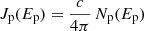 is the (isotropic) proton flux (with Np(Ep) the proton spectrum given by Eq. 4), dσ(Eπ0, Ep)/dEπ0 is the differential cross-section for production of neutral pions with energy Eπ0 from a collision of a proton with energy Ep with an ambient proton (essentially at rest), and
 ![$ E^{thr}_{\mathrm{p}} = m_{\mathrm{p}}\,[1+({m_\pi^0}^2+4 m_{\mathrm{p}} m_\pi^0)/(2m_{\mathrm{p}}^2)] = 1.22 $](/articles/aa/full_html/2024/05/aa47976-23/aa47976-23-eq72.gif) GeV is the threshold energy for
GeV is the threshold energy for  production. We applied a δ-function approximation (Aharonian & Atoyan 2000) to the differential cross-section by assuming that a fixed average fraction, κπ0 (≃0.17 in the GeV-TeV region), of the proton kinetic energy,
 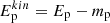 , is transferred to the neutral pion, namely,
  , where σpp is the inclusive total cross-section for inelastic p-p collisions (i.e. it contains the multiplicity of the pions produced in each hadronic interaction; e.g. Dermer 1986; Achilli et al. 2011; Aaij et al. 2015). The latter cross-section can be analytically approximated as (Kelner et al. 2006, Eq. 79)
![$$ \begin{aligned} \sigma _{pp}(E_{\rm p}) ~=~ \left[ 34.3 + 1.88\,\mathrm{ln}\left({E_{\rm p} \over \mathrm{TeV}}\right) + 0.25\,\left[\mathrm{ln}\left({E_{\rm p} \over \mathrm{TeV}}\right)\right]^2 \right] ~ \left[1 - \left( {E_{\rm thr} \over E_{\rm p}} \right)^4 \right]^2 \mathrm{mbarn} \,, \end{aligned} $$](/articles/aa/full_html/2024/05/aa47976-23/aa47976-23-eq76.gif)
leading to

The resulting γ-ray photon emissivity is

A.2.2. Secondary electrons and positrons from π± decay
The production rate of (secondary) electrons and positrons (hereafter collectively called ’electrons’) is calculated from the π± decay rate density (e.g. Stecker 1971):

where fπ±, p(Ep, Eπ±) is the π± energy distribution for an incident proton energy Ep. The π± energy distribution can be well approximated by assuming that a constant fraction, kπ±, of the proton kinetic energy is transferred to charged pions, so that

where σpp(Ep) is the total inclusive cross-section of inelastic p-p collisions (see above). For the range of qp values of interest here, kπ± = 0.25 (Kelner et al. 2006). Substituting Eq. (A.20) in Eq. (A.19) we obtain

Next, we calculate the source spectrum of secondary electrons, Qse(γ) (Gould & Burbidge 1965; Ramaty & Lingenfeltern 1966). In the muon (∼ pion) frame, the secondary-electron distribution is:
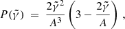
where  , which reaches a maximum of A = 105 (corresponding to 52 MeV), is the (secondary) electron Lorentz factor in the muon frame. Then,
  can be approximated by a delta function around
 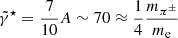 , that is:
 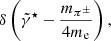 where δ(x) is the Dirac δ-function. Since
  (Scanlon & Milford 1965), at high energies
 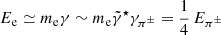 . The e±-source spectrum is then Qse(Ee) = ∫Qπ±(Eπ±) δ(Ee − Eπ±) dEπ± = Qse(Ee) = 4 Qπ±(4Ee); combining the latter with Eqs. (A.21) and (A.16) and expressing electron energies as a function of the electron Lorentz factor γ, in the laboratory frame the secondary-electron injection spectrum is 21

where 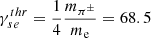 and
and 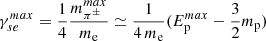 .
.
Finally, the corresponding steady-state distribution, Nse(γ), can be calculated from the kinetic equation
![$$ \begin{aligned} {d \left[b(\gamma ) N_{se}(\gamma ) \right] \over d\gamma } ~=~ Q_{se}(\gamma ),\, \end{aligned} $$](/articles/aa/full_html/2024/05/aa47976-23/aa47976-23-eq92.gif)
where, assuming transport losses to be negligible, b(γ) is the radiative energy loss term. In a medium that consists of ionised, neutral, and molecular gas with densities ni, nHI, and nH2, respectively, the loss term is written as b(γ) = b0(γ)+b1(γ)+b2(γ), where:
![$$ \begin{aligned} - b_0(\gamma ) = 1.1 \cdot 10^{-12} \, \sqrt{1-\gamma ^{-2}} \, \left[ n_{\rm i} \, \left( 1 - \frac{\mathrm{ln} \, n_{\rm i}}{74.6} \right) + 0.4\,(n_H+2n_{H2}) \right] \mathrm{s}^{-1}, \, \end{aligned} $$](/articles/aa/full_html/2024/05/aa47976-23/aa47976-23-eq93.gif)
![$$ \begin{aligned} - b_1(\gamma ) = 1.8 \cdot 10^{-16} \gamma \,\left[n_{\rm i} + 4.5\,(n_H+2n_{H2})\right] \mathrm{s}^{-1}, \, \end{aligned} $$](/articles/aa/full_html/2024/05/aa47976-23/aa47976-23-eq94.gif)

These are the loss rates by, respectively, electronic excitations in ionised gas, electron bremsstrahlung in ionised gas (strong shield limit), and synchrotron-Compton radiation in the ambient magnetic and radiation field energy (ρr) densities. For a discussion of the bj(γ) terms, we refer to Rephaeli & Persic (2015). The secondary electron spectrum is then:
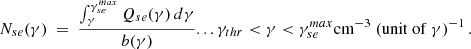
In the radiative-yield calculations, Nse(γ) can be numerically approximated as
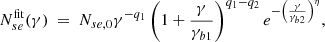
where q1 and q2 are the low- and high-frequency slopes, b1 and b2 are the low- and high-frequency breaks, and η is a parameter describing the sharpness of the high-energy spectral cutoff.
A.2.3. Neutrinos from π± decay
Here, we summarise (from Kelner et al. 2006) the spectral properties of the decay neutrinos of ultrarelativistic charged pions. We set x ≡ Eν/Eπ±, 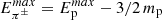 , and Θ(x) the Heaviside function (Θ(x) = 1 if x ≥ 0, and Θ(x) = 0 if x < 0) throughout.
• π → μνμ. In the laboratory frame, a pion of energy Eπ± > > mπ emits a νμ whose energy appears in the range 0 ≤ Eν ≤ λEπ (where 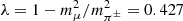 ) with constant probability. The energy probability distribution for a single emitted neutrino is
and the injection spectrum of pion-decay muon neutrinos is

where the factor 2 accounts for the contributions from both π+ and π− pions.
• μ → e νe νμ. In the laboratory frame, the energies of the neutrinos produced through the decay of secondary muons appear in the range of 0 ≤ x ≤ 1, according to probability distributions given, for νμ and νe, respectively, (setting r ≡ 1 − λ = 0.573) as follows:
![$$ \begin{aligned} f_{\nu _\mu ^{(2)}}(x) = g_{\nu _\mu }(x) \Theta (x-r) \, + \, \left[ h_{\nu _\mu }^{(a)}(x) + h_{\nu _\mu }^{(b)}(x) \right] \Theta (r-x) \,, \end{aligned} $$](/articles/aa/full_html/2024/05/aa47976-23/aa47976-23-eq102.gif)
where
![$$ \begin{aligned} h_{\nu _\mu }^{(b)}(x) = \frac{(1+2r)(r-x)}{9 r^2} \,\left[ 9\, (r+x) - 4(r^2 + rx + x^2) \right] \,; \end{aligned} $$](/articles/aa/full_html/2024/05/aa47976-23/aa47976-23-eq105.gif)
and
![$$ \begin{aligned} f_{\nu _{\rm e}}(x) = g_{\nu _{\rm e}}(x) \Theta (x-r) \, + \, \left[ h_{\nu _{\rm e}}^{(a)}(x) + h_{\nu _{\rm e}}^{(b)}(x) \right] \Theta (r-x) \,, \end{aligned} $$](/articles/aa/full_html/2024/05/aa47976-23/aa47976-23-eq106.gif)
where
![$$ \begin{aligned} g_{\nu _{\rm e}}(x) = \frac{2}{3\,(1-r)^2} \,\left[ (1-x) \left(6\,(1-x)^2 + r\,(5+5x-4x^2) \right) + 6r\, \mathrm{ln}\,x \right], \end{aligned} $$](/articles/aa/full_html/2024/05/aa47976-23/aa47976-23-eq107.gif)
![$$ \begin{aligned} h_{\nu _{\rm e}}^{(a)}(x) = \frac{2}{3\,(1-r)^2} \,\left[ (1-r)\,(6-7r+11 r^2 - 4 r^3) + 6r\, \mathrm{ln}\,r \right], \end{aligned} $$](/articles/aa/full_html/2024/05/aa47976-23/aa47976-23-eq108.gif)

The probability distribution functions in Eqs. A.30, A.32, and A.36 are normalised, as per  . The corresponding injection spectra for μ-decay muon and electron neutrinos are, respectively,

and

In Eqs. A.40 and A.41, the factor of 2 accounts for the contributions from both the π+ and π− pions.
Appendix B: Notes on Table 4
• M31. Neutral and molecular gas densities are derived from HI and H2 surface densities (Fig. 12 of Nieten et al. 2006) using a constant vertical scale height (hs = 0.24 kpc) crossing the galactic midplane (Brinks & Burton 1984). The hot ionised plasma density is derived from X-ray measurements: ni ∼ f−1/210−2 ≃ 0.04 cm−3, assuming a filling factor f ∼ 0.1 (Kavanagh et al. 2020). The Hα emission measure, EM, is deduced from Walterbos & Braun (1994).
• M33. Neutral and molecular gas densities are inferred from the corresponding masses, MHI = 1.9 109 M⊙ and MH2 = 3.3 108 M⊙ (Abdo et al. 2010), for the assumed sizes. The ionised gas density is inferred from the diffuse Hα emission, 0.03 ± 0.03 cm−3 (Tabatabaei et al. 2008), thermal X-ray luminosity (Schulman & Bregman 1995) and temperature (Long et al. 1996), and the estimated emission region, ∼0.01 cm−3. Finally, the Z2, EM is from Monnet (1971).
The quantity Z2 ≡ ne/ni in the hot diffuse ionised plasma, measured by Kavanagh et al. (2020) as 1.21 in M31, is assumed to have the same value in M33. It should be noted that the same value is also measured in the Magellanic Clouds (Sasaki et al. 2002). The assumed warm-plasma temperature,  , is standard for H II regions.
All Tables
All Figures
|
Fig. 1. γ-ray spectrum of emission from the central source of M31, |
| In the text | |
|
Fig. 2. Radio spectrum of M31. The data points (from Battistelli et al. 2019) denote the whole-galaxy radio flux reduced to the estimated flux expected from within the R⋆ radial region as described in the text. Also shown are: (top) Battistelli et al. (2019) fit (single electron population synchrotron: dotted curve; thermal free–free emission: dot-dashed curve), and (bottom) our LH emission model. The latter includes primary and secondary synchrotron radiation (dotted curves of increasing flux at their peaks) and a thermal free–free component (dot-dashed curve). |
| In the text | |
|
Fig. 3. Broadband lepto-hadronic SED of the M31 central source: data points are shown as dots (with errorbars indicating frequency and flux uncertainties), model predictions as curves (top). The galaxy-wide flux densities of Battistelli et al. (2019) have been renormalised to the region encompassed by R⋆ (i.e., ∼15% of the total emission; see Sect. 4.1.2). Emission components are denoted by these line types: radio synchrotron, dotted; thermal free–free emission, dot-dashed; total radio, solid; Comptonised CMB, short-dashed; Comptonised starlight (EBL+FGL), long-dashed; non-thermal bremsstrahlung, dotted; pionic, solid. Leptonic emission includes that from primary and secondary electrons(secondary components are dominant). In the X-ray/γ-ray range, on top of the separate components, a thick solid line indicates the total emission. Same for a broadband PSR+LH SED (middle). The 500 pulsars emission component (see text) is ahown as a dot-dashed line. Same as above but for 1000 pulsars (bottom). Note: in this case the secondary leptonic components are subdominant. |
| In the text | |
|
Fig. 4. SED of M33. Radio spectrum (top): the emission model (solid curve), including primary and secondary synchrotron radiation (dotted curves of decreasing flux) as well as a thermal free–free component (dot-dashed curve), is overlaid with data from Table 2 (black dots). The empty squares represent the estimated radio flux after removing the contribution from ≤200 pc size sources (Tabatabaei et al. 2022). The total radio emission, resulting if the ‘nominal’ primary electron spectrum is used, is indicated by the dashed curve. Broadband SED (bottom): data points are shown as dots, model predictions as curves. Emission components are plotted by the following line types: radio synchrotron, dotted; thermal free–free emission, dot-dashed; total radio, solid; Comptonised CMB, long-dashed; Comptonised starlight (EBL+FGL), short-dashed; non-thermal bremsstrahlung, dotted; and pionic, solid. For each type of non-thermal leptonic yield, the total, primary, and secondary emissions are denoted as curves of progressively lower flux. In the X-ray and γ-ray range, on top of the separate components, a solid line indicates the total emission. The empty squares and dashed curve in the radio are as described in the top panel. |
| In the text | |
Current usage metrics show cumulative count of Article Views (full-text article views including HTML views, PDF and ePub downloads, according to the available data) and Abstracts Views on Vision4Press platform.
Data correspond to usage on the plateform after 2015. The current usage metrics is available 48-96 hours after online publication and is updated daily on week days.
Initial download of the metrics may take a while.