| Issue |
A&A
Volume 666, October 2022
|
|
|---|---|---|
| Article Number | A167 | |
| Number of page(s) | 11 | |
| Section | Interstellar and circumstellar matter | |
| DOI | https://doi.org/10.1051/0004-6361/202243391 | |
| Published online | 25 October 2022 | |
Diffuse non-thermal emission in the disks of the Magellanic Clouds
1
INAF/Trieste Astronomical Observatory,
via G.B. Tiepolo 11,
34100
Trieste, Italy
INFN-Trieste,
via A.Valerio 2,
34127
Trieste, Italy
e-mail: massimo.persic@inaf.it
2
School of Physics & Astronomy, Tel Aviv University,
Tel Aviv
69978, Israel
Center for Astrophysics and Space Sciences, University of California at San Diego,
La Jolla, CA
92093, USA
e-mail: yoelr@wise.tau.ac.il
Received:
22
February
2022
Accepted:
28
July
2022
Context. The Magellanic Clouds, two dwarf galaxy companions to the Milky Way, are among the Fermi Large Area Telescope (LAT) brightest γ-ray sources.
Aims. We present comprehensive modeling of the non-thermal electromagnetic and neutrino emission in both Clouds.
Methods. We self-consistently model the radio and γ-ray spectral energy distribution from their disks based on recently published Murchison Widefield Array and Fermi/LAT data. All relevant radiative processes involving relativistic and thermal electrons (synchrotron, Compton scattering, and bremsstrahlung) and relativistic protons (neutral pion decay following interaction with thermal protons) are considered, using exact emission formulae.
Results. Joint spectral analyses indicate that radio emission in the Clouds has both primary and secondary electron synchrotron and thermal bremsstrahlung origin, whereas γ rays originate mostly from π0 decay with some contributions from relativistic bremsstrahlung and Comptonized starlight. The proton spectra in both galaxies are modeled as power laws in energy with similar spectral indices, ~2.4, and energy densities, ~1 eV cm−3. The predicted 0.1–10 GeV neutrino flux is too low for detection by current and upcoming experiments.
Conclusions. We confirm earlier suggestions of a largely hadronic origin of the γ-ray emission in both Magellanic Clouds.
Key words: radiation mechanisms: non-thermal / Magellanic Clouds / gamma rays: galaxies / radio continuum: galaxies / astroparticle physics / acceleration of particles
© M. Persic and Y. Rephaeli 2022
 Open Access article, published by EDP Sciences, under the terms of the Creative Commons Attribution License (https://creativecommons.org/licenses/by/4.0), which permits unrestricted use, distribution, and reproduction in any medium, provided the original work is properly cited.
This article is published in open access under the Subscribe-to-Open model. Subscribe to A&A to support open access publication.
1 Introduction
The spectral energy distributions (SEDs) of cosmic rays (CRs) outside their galactic accelerators are important for determining basic properties of CR populations and for assessing the impact of the particle interactions in the magnetized plasma in galactic disks and halos. Knowledge of these distributions is generally limited as it is usually based only on spectral radio observations. When, in addition, non-thermal (NT) X/γ-ray observations are available, reasonably detailed spectral modeling of the CR electron (CRe) and proton (CRp) distributions in star-forming environments can be very useful. Sampling the SED over these spectral regions yields important insight into the emitting CRe and possibly also CRp, whose interactions with the ambient plasma may dominate (via π0 decay) high-energy emission (≳100MeV).
The nearby Magellanic Clouds (MCs), two irregular dwarf satellite galaxies of the Milky Way, may exemplify the level of spectral modeling currently feasible in a joint analysis of radio and γ-ray measurements. The Large MC (LMC) is located at a distance d = 50 kpc (Foreman et al. 2015); for the purpose of this study, its structure is modeled as a cylinder with radius r = 3.5 kpc and height h = 0.4 kpc (Ackermann et al. 2016).
Similarly, for the Small MC (SMC) these quantities are d = 60 kpc, r = 1.6 kpc, and h = 4 kpc (Abdo et al. 2010b).
Both MCs have been detected with the Fermi Large Area Telescope (LAT) as extended sources (Abdo et al. 2010a,b). Based on recent data (Lopez et al. 2018), there is statistically significant emission along the SMC “bar” and “wing” where there is active star formation. A spectro-spatial analysis of the LAT data suggests its integrated γ-ray emission to be mostly hadronic (≥90%). Similar analyses of the LMC with multi-source models (Foreman et al. 2015; Ackermann et al. 2016; Tang et al. 2017) attempted to extract the spectral content of these sources in a statistically viable way (including details on the quality of the fits). The sources were found to be point-like (pulsars, supernova remnants, plerions, unidentified background active galactic nuclei) and extended. The extended sources included the large-scale disk denoted as1 E0 ~ G1, and smaller-scale components denoted as E1+E3 ~ G2 (the region west of 30 Doradus); E2 ~ G3 (the LMC northern region); and E4 ~ G4 (the LMC western region) – these smaller-scale components possibly encompass different sources with different spectra. These spectral and/or spatial analyses revealed a galaxy-scale component dominating the emission, with a spectral shape suggesting a lepto-hadronic (Foreman et al. 2015) or hadronic (Ackermann et al. 2016; Tang et al. 2017) origin2.
In this paper, we focus on the emission in the MC disks in an attempt to determine the mean values of their magnetic fields and CRe and CRp energy densities. In spite of their detailed LAT data analyses, the above-mentioned studies were not based on self-consistent modeling of the broadband radio-γ SED of the two galaxies. SED modeling is important because a firm proof of the (mostly) pionic nature of the γ-ray emission should be based on a quantitative estimate of the CRe spectrum. Clearly, this spectrum is primarily determined from measurements of synchrotron radio emission, which was not accounted for in the earlier works. In an attempt to clarify, and possibly remove, some uncertainties inherent in previous modeling work, here we reassess key aspects of (average) conditions in the MC large-scale disks. Employing a one-zone model for the extended disk emission, we self-consistently carry out detailed calculations of the emission by CRe and CRp. The radio and γ-ray data used in our analyses are taken from the following papers: Lopez et al. (2018, SMC), Tang et al. (2017, LMC), Ackermann et al. (2016, LMC), and Alvarez et al. (1987, SMC, LMC).
In Sect. 2, we briefly review the observations of extended NT emission from the MC disks. In Sect. 3, we review the IR-optical radiation fields permeating the MCs. In Sect. 4, we describe calculations of the MC disk SEDs and perform fits to the data. Prospects of neutrino detection are discussed in Sect. 5, followed by a conclusion in Sect. 6.
SMC radio and γ-ray data.
2 Observations of extended emission
The MCs have been extensively observed over a wide range of radio-microwave, (soft) X-ray, and γ-ray bands. As mentioned above, point-source emission and extended small- and large-scale emission have been detected from both galaxies. In this paper we focus on the extended large-scale disk emission of each galaxy because this emission traces the mean galactic properties of NT particles and magnetic fields. The spectral datasets used in our analysis are public (either tabulated or plotted) and are fully specified in Table 1 (SMC) and Table 2 (LMC). In this section we briefly review the observations most relevant to NT emission leaving out details that are discussed in the cited papers.
Radio. In a multifrequency radio continuum study of the MCs, For et al. (2018) presented closely-sampled 76–227 MHz Murchison Widefield Array data, supplemented by previous radio measurements at lower (for the LMC) and higher (for both MCs) frequencies. Measured fluxes include emission from MC (and background) point sources, which were estimated to contribute 11% and 23% of the measured emission of the SMC and the LMC, respectively. Based on statistical analyses of a set of four fitting spectral models (power-law [1PL], curved PL, and double PL [2PL]) with either free and fixed high-v index), they found that for the SMC the best-fitting model is a 1PL (in the 76–8550 MHz band) with α(85.5MHz–8.55 GHz) = 0.82 ± 0.03 (consistent with Haynes et al. 1991). Instead, for the LMC the preferred model is a 2PL (19.7-8550 MHz) with a low-v (19.7–408 MHz) index α0 = 0.66 ± 0.08 (consistent with Klein et al. 1989) and a (fixed) high-v index α1 = 0.1 suggesting that synchrotron radiation and thermal free-free (ff) emission dominate at low and high frequencies, respectively.
X-rays. The observed diffuse X-ray emission in the MCs has been determined to be of thermal origin (Wang et al. 1991: Einstein Observatory; Points et al. 2001: Röntgen Satel-lit (ROSAT) Position Sensitive Proportional Counters (PSPC); Nishiuchi et al. 1999, 2001: Advanced Satellite for Cosmology and Astrophysics (ASCA)); as such, it is not directly relevant to our SED analysis except for the estimated thermal plasma density, which is required to calculate the pionic emission (see below).
Gamma rays. Both MCs were detected at > 100 MeV γ rays as galaxy-scale extended sources whose emission is dominated by a diffuse component. This component has been interpreted as mainly originating from CRp interacting with the interstellar gas.
The SMC was first detected with 17 months of Fermi/LAT data (Abdo et al. 2010b) as a ~3°-size source, in which emission was not strongly correlated with prominent sites of star formation. More recently Lopez et al. (2018), based on 105 months of LAT Pass8 data, produced maps of the extended >2GeV emission (no signal at > 13 GeV) and found statistically significant emission along the galaxy-scale quietly star-forming bar and wing. Within a set of single-component spectral models (i.e., PL; broken PL, with frozen spectral shape and free normalization, representing pulsars; and exponentially cutoff PL, representing pionic emission) the exponentially cutoff PL provides the best fit to the total γ-ray spectrum, with only a marginal improvement of the fit if the broken PL is added. citepbib21 analysis suggests that although pulsars may contribute ≤10% at > 100 MeV, the extended emission is mainly (≥90%) of pionic origin, with a γ-ray emissivity ≳5 times smaller than the local (Galactic) emissivity.
The LMC was marginally (>4.5 σ) detected with the Compton Gamma Ray Observatory (CGRO) Energetic Gamma Ray Telescope (EGRET; Sreekumar et al. 1992) and then confirmed (33 σ) with 11 months of Fermi/LAT data (Abdo et al. 2010a).
More recent studies have focused on the spatial and spectral modeling of the γ-ray surface brightness distribution; these are briefly reviewed below.
The first LAT-based spectro-spatial analysis of the γ-ray surface brightness distribution was performed by Foreman et al. (2015) using 5.5 yr of data, in the photon energy range 0.220 GeV. They modeled the CR distribution and γ-ray production based on observed maps of the LMC interstellar medium, star formation, radiation fields, and radio emission. The γ-ray spectrum was described by means of analytical fitting functions for the π0-decay, bremsstrahlung, and inverse-Compton yields. These processes were estimated to account for, respectively, 50%, 44%, and 6% of the total 0.2–20 GeV emission. In particular, they inferred the CRp spectral index to be qp = 2.4 ± 0.2 and the equipartition (with CRp) magnetic field to be Beq = 2.8 µG.
A subsequent spectro-spatial analysis (Ackermann et al. 2016, A+16) of 6yr of LAT (P7REP) data in the 0.2–100 GeV band reported extended and point-like emissions. The dominant extended emission is in the form of a disk-scale component, denoted as E0 in their paper, and additional degree-scale emissions from several regions of enhanced star formation (including 30 Doradus). If pionic, the E0 emission component implies a population of CRp with ~1/3 the local Galactic density, whereas the superposed small-scale emissions imply local enhancements of the CRp density by factors of at least 2–6. The spectrum of the E0 component (which does not include emission from the degree-scale emissions from several regions) shows some curvature (see their Fig. 7, top): with no reference to the underlying emission mechanism, A+16 fitted the data with a tabulated function derived from the local (Galactic) gas emissivity spectrum (as a result of its interactions with CRp), an exponentially cutoff PL, a broken PL, and a log-parabola, and concluded that the best-fitting analytical model was the log-parabola. They noted, however, that the similarity between the log-parabola and tabulated-function models (see their Fig. 9) suggests a pionic nature of the large-scale disk emission.
More recently Tang et al. (2017, T+17) analyzed 8 yr of LAT Pass8 data and deduced a deeper, more spectrally extended 0.0880 GeV spectrum of the large-scale disk component (identified as G1; this too did not include emission from other regions) largely overlaps with E0 of A+16. The G1 shape, now extending down to 60 MeV, was determined to be best described as a π0 - decay hump from a CRp spectrum harder than that in our Galaxy, although they could not rule out CRe relativistic bremsstrahlung completely. In this analysis we use the T+17 G1 data as our reference set for the diffuse large-scale LMC disk emission, and the earlier A+16 E0 data as an auxiliary set for a consistency check.
LMC radio and γ-ray data.
3 Radiation fields
A reasonably precise determination of the ambient radiation field is needed to predict the level of γ-ray emission from Compton scattering of target photons by the radio-emitting electrons (and positrons). The total radiation field includes cosmic (background) and local (foreground) components.
Relevant cosmic radiation fields include the cosmic microwave background (CMB) and the extragalactic background light (EBL). The CMB is a pure Planckian described by a temperature TCMB = 2.735(1 + z)K and energy density uCMB = 0.25 (1 + z)4 eV cm−3. The EBL originates from direct and dust-reprocessed starlight integrated over the star formation history the Universe. It shows two peaks, corresponding respectively to the cosmic infrared background (CIB, at ~100 µm) that originates from dust-reprocessed starlight, and the cosmic optical background (COB, at ~1 µm) that originates from direct starlight (e.g., Cooray 2016). The two peaks are described as diluted Planckians, characterized by a temperature T and a dilution factor Cdii. The latter is the ratio of the actual energy density, u, to the energy density of an undiluted blackbody at the same temperature, T (i.e., u = Cdil aT4, where a is the Stefan-Boltzmann constant). The dilution factors of the cosmic fields are CCMB = 1, CCIB = 10−5.629, and CCOB = 10−13.726. A recent updated EBL model, based on accurate galaxy counts in several spectral bands, is due to Franceschini & Rodighiero (2017); locally (z = 0) it can be numerically approximated as a combination of diluted Planckians,

with A1 = 10−5.629, T1 = 29 K; A2 = 10−8.522, T2 = 96.7 K; A3 = 10−10.249, T3 = 223 K; A4 = 10−12.027, T4 = 580 K; A5 = 10−13.726, T5 = 2900 K; A6 = 10−15.027, T6 = 4350 K; A7 = 10−16.404, T7 = 5800 K; A8 = 10−17.027, T8 = 11600 K.
Local radiation fields in the MCs arise from their intrinsic stellar populations and (given its close proximity) also from the Milky Way; we refer to this as the galactic foregound light (GFL). Similar to the EBL by shape and origin, the GFL is dominated by two thermal humps, IR and optical. The corresponding energy densities (in eV cm−3) are (i) LMC: uIR = 0.12 and uopt = 0.20, estimated from Foreman et al. (2015, uIR+opt = 0.32) and the IR-opt SED (from NED3); (ii) SMC: uIR = 0.026, uopt = 0.062, scaling down the LMC values taking (from the SED, cf. NED) the optical and IR peaks to be factors of 0.215 and 0.144, respectively, of the corresponding LMC values.
4 SED models
Our main objective in this study is to determine CR electron and proton spectra in the MC disks by spectral modeling of NT emission in all the relevant energy ranges accessible to the observations. The particle, gas density, magnetic, and radiation field distributions clearly vary significantly across the disk, obviating the need for a spectro-spatial treatment. A modeling approach based on a solution to the diffusion-advection equation has been applied in the study of the Galaxy and several nearby galaxies. However, even for just a diffusion-based treatment to be feasible and meaningful, the spatial profiles of key quantities, such as the particle acceleration sources, gas density, magnetic field, and generally also the diffusion coefficient have to be specified. Given the generally very limited observational basis for reliably determining these profiles, a parameter-intensive spectro-spatial modeling approach is rarely warranted. An example is the very approximate diffusion-based approach adopted in modeling NT emission in the disks and halos of the star-forming galaxies NGC 4631 and NGC 4666 (Rephaeli & Sadeh 2019) for which reasonably detailed radio spectra and spatial profiles are available; even so, the results of these analyses are not conclusive given the substantial uncertainty in the values of key parameters.
Radio emission in the MC disks is electron synchrotron in a disordered magnetic field whose mean value B is taken to be spatially uniform, and thermal ff from a warm ionized plasma. A significant CRp component could yield additional radio emission by secondary e± produced by π± decays, and γ-ray emission from π0 decay. In addition, γ-ray emission is produced by CRe scattering off photons of local and background radiation fields. The calculations of the emissivities from all these processes are well known and standard.
We assume the CR spectral distributions to be time-independent and locally isotropic with spectral PL form. The primary CRe spectral density (per cm3 and per unit of the electron Lorentz factor γ) is, Ne(γ) = Ne,0 γ−qe
for γmin < γ < γmax with γmin ≫1. As discussed later, this spectrum proves to be a good approximation to the actual primary steady-state spectrum in the relevant electron energy range. The secondary CRe spectrum can be analytically approximated as a smoothed 2PL, exponentially cut off at high energies (see below). The assumed CRp spectrum (in units of cm−3 GeV−1) as a function of Ep/GeV is, Np(Ep) = Np,0  for
for  .
.
4.1 SMC
The emission spectrum from π0-decay has more constraining power than a generic PL; thus, our modeling procedure begins with fitting a pionic emission profile to the γ-ray data with free normalization, slope, and high-energy cutoff. We then use the deduced (essentially, fully determined) secondary CRe spectrum together with an assumed primary CRe spectrum to calculate the combined synchrotron emission using an observationally estimated value of B. The fit to the radio data also includes, at high frequencies, a thermal bremsstrahlung component computed with previously determined values of the gas density and temperature. Finally, the full Compton X-ray and γ-ray yield is determined.
The π0-decay γ-ray flux is computed using the emissivity in Eq. (15) of Persic & Rephaeli (2019a), where the total (thermal) gas proton density is  with the average neutral-hydrogen density nHI = 0.54 cm−3, inferred from MHI = 4.23 × 10⁸ M⊙ (this value of MHI was deduced from direct determination of HI column density from the 21 cm emission line; Stanimirovic et al. 1999), and the molecular-hydrogen density
  = 0.02 cm−3, inferred from
  = 3.2 × 10⁷ M⊙ (which, in turn, is derived from modeling Spitzer, Cosmic Background Explorer (COBE), InfraRed Astronomical Satellite (IRAS), and Infrared Space Observatory (ISO) far-infrared data; Leroy et al. 2007). The CRp spectrum derived from our fit to the Fermi/LAT data is Np0 = 2.4 × 10⁻¹⁰ cm−3, qp = 2.40, with
  = 30 GeV. The model spectrum fully reproduces the 0.2–50 GeV Fermi/LAT spectrum (Fig. 1). With these values, the estimated CRp energy density
  Ep Np(Ep) dEp is ~0.5 eV cm−3.
The closely related π± -decay secondary CRe spectrum, Nse(γ), has no free parameters once the CRp spectrum is determined4. We use  , with parameter values reported in Table 3, to compute the corresponding leptonic yields. However, the uncertainty in the total (HI and H2) gas density clearly affects the energy loss rate b(γ) and the resulting spectral normalization and shape of Nse(γ), hence also of Ne(γ), and their yields. To compute the synchrotron emission we assume B = 3.5 µG, based on estimates of the ordered (1.7 µG) and random (3 µG) fields in the SMC (Mao et al. 2008).
Once the secondary CRe synchrotron yield has been computed, its low-frequency residuals from the data are modeled using a CRe spectrum, Ne(γ), with Ne0 = 3.7 × 10⁻⁸ cm−3, qe = 2.23, γmax = 104. This spectrum is the 1PL approximation, for 100 ≲ γ ≲ γmax, of the actual steady-state primary CRe spectrum. Neglecting diffusion and advection losses, this primary spectrum is ![${N_{{\rm{p}}e}}\left( \gamma \right) = {k_i}{\gamma ^{ - \left( {{q_i} - 1} \right)}}/\left[ {b\left( \gamma \right)\left( {{q_i} - 1} \right)} \right]$](/articles/aa/full_html/2022/10/aa43391-22/aa43391-22-eq20.png) cm−3 (units of γ)−1 where
cm−3 (units of γ)−1 where  is the CRe spectral injection rate. Over the mentioned electron energy range, we find that qi = 2.28 provides a decent match between the shapes of the curved spectrum and the 1PL spectrum; this value is typical for γ-ray emission from Galactic CR accelerators (e.g., supernova remnants, the Crab nebula). The relative normalization between the two spectra can be based on the measured flux density at some radio frequency or on imposing the same CRe energy density on the two spectra over the electron energy range of interest (see discussion in Rephaeli & Persic 2015). In our case the normalization of Npe(γ), and hence ki, can be found by using both Npe(γ) and Nse(γ) to compute the total (primary plus secondary) synchrotron yield, which in turn is fitted to the radio synchrotron data. In doing this, the acceptable match (in the relevant energy range) between the curved and PL spectra allows us to use Ne(γ) without substantial loss of accuracy. Given this procedure, the uncertainties in the gas density ultimately affect Ne(γ) as well.
The spectra of the synchrotron-emitting CRe are shown in Fig. 2. The resulting primary electron component is quite dominant, with ~70% of the total synchrotron and Compton yields (Fig. 3), but the normalization, Ne0, is not strongly constrained due to its dependence on the assumed magnetic field. If measurements of NT-X-ray and ~1–30MeV γ-ray fluxes, which correspond respectively to the CMB and CIB peaks, become available, most of the uncertainty could be removed (e.g., Persic & Rephaeli 2019a). In addition to this modeling uncertainty, the considerable coupling between the CRe spectral parameters implies an appreciable range of the deduced values of Ne0 and qe. This range can be roughly bracketed by a flatter slope (qe = 2.2) and lower normalization (Ne0 = 2.9 × 10⁻⁸ cm−3) or, alternatively, a steeper slope (qe = 2.3) and higher normalization (Ne0 = 6.7 × 10⁻⁸ cmv3), both with the same γmax as the reference model (Table 3).
At high frequencies a relatively flat, ∝v−0.1, component represents diffuse thermal ff emission (Spitzer 1978). This flux may be gauged to the Hα flux if both emissions come from the same emitting volume (HII regions) because in this case the relevant warm-plasma parameters (temperature, density, filling factor) are the same. So the measured (optical) Hα flux may be used to predict the (radio) ff emission. We model the thermal ff emission combining Eqs. (3) and (4a) of Condon (1992) and using Te = 1.1 × 10⁴ K (Toribio San Cipriano et al. 2017) and F(Hα) = 1.6 × 10⁻⁸ erg cm−2 s−1 (Kennicutt et al. 1995). The primary synchrotron and thermal ff normalizations are spectrally quite far apart so they do not significantly affect each other. The radio model is shown alongside data in Fig. 3-right.
Although they are subdominant, secondary CRe contribute appreciably to the total CRe population of the SMC. Whereas the primary spectrum is approximately PL, the secondary spectrum is clearly curved (see Fig. 2). The resulting curvature of the total CRe spectrum is reflected in the total synchrotron spectrum (computed using Eq. (9) of Persic & Rephaeli 2019a for Ne(γ) and its straightforward generalization for Nse(γ)). Therefore, the total radio spectrum, which consists of synchrotron and thermal ff emission at low and high frequencies, is not a smooth 2PL, but shows some extra structure. A third-order polynomial (in log units) outperforms the For et al. (2018) “preferred” 1PL model (∆BIC > 0; Table 4). This polynomial (four free parameters; Fig. 3-left) is matched by the physical model described above, namely a low-frequency component representing synchrotron emission (three free parameters) plus a high-frequency ∝ ν−0.1 PL representing thermal ff emission (one free parameter; Fig. 3-right).
With the CRe spectra essentially determined, we can calculate the Compton and NT-bremsstrahlung yields from CRe scattering off, respectively, CMB-EBL-GFL photons and thermal plasma nuclei using, respectively, Eqs. (2.42) and (3.1) of Blumenthal & Gould (1970). The photon fields are described in Sect. 3; for the plasma nuclei we assume a density ni = 0.033 cm−3 (Mao et al. 2008) and metallicity Z2 = 1.2 (Sasaki et al. 2002). Although the shape of the γ-ray spectrum is distinctly pionic, NT-bremsstrahlung peaks near the pionic peak (ν ~ 1023 Hz) where it contributes ~3% of the measured flux; Comptonized starlight (EBL+GFL) emission, which peaks at ν ~ 1022 Hz, contributes ≲1% of the flux at the lowest LAT data point. The predicted Comptonized CMB spectral flux is also shown in Fig. 4. We found no need to introduce a further broken PL component in the γ-ray band representing pulsars, in agreement with Lopez et al. (2018). The resulting SED model, overlaid on data, is plotted in Fig. 4.
An upper limit on the mean magnetic field, Bmax, can be estimated by assuming that the measured radio emission is fully produced by secondary CRe. By matching the measured and predicted emission levels we infer a limiting value Blim ≃ 7 µG. This upper limit, which is twice the observationally deduced value, is unrealistically high because the shapes of the measured and predicted synchrotron spectra do not match well, most notably at low frequencies, and because primary CRe obviously contribute to the measured radio flux. A lower limit, Bmin, can estimated using the fact that if B decreases the secondary synchrotron yield decreases as well. In order to keep the synchrotron yield unchanged, the primary yield must increase by increasing the spectral normalization (Ne0) and possibly also varying the spectral shape (qe, γmax) of the primary CRe spectrum. At low energies the primary spectrum is steeper than the secondary, which means that at some point the resulting synchrotron spectrum becomes progressively and systematically steeper than the <230 GHz radio data; this yields Bmin ≃ 2 µG. Based on our SED analysis, the value B = 3.5 µG suggested by Mao et al. (2008) lies comfortably between the estimated bounds.
SED model parameters.
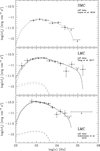 |
Fig. 1 Gamma-ray spectra in the Magellanic Clouds. Curves represent: (top) pionic emission, solid; (middle and bottom, in decreasing flux): total gamma and pionic emissions, solid, and total and primary NT bremsstrahlung, dashed. |
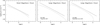 |
Fig. 2 CRe spectra in the Magellanic Clouds. The curves are the secondary spectra (dashed), primary spectra (dotted), and the primaries’ local PL representations (solid). In each panel the normalization of the primary CRe spectrum to its PL counterpart is chosen such that they nearly overlap. The primary CRe injection indices, qi, are 2.28 (SMC) and 2.23 (LMC). The two LMC CRe spectra panels refer, respectively, to the T+17 and A+16 Fermi/LAT datasets, as secondary spectra are derived from the pionic fits to the γ-ray data. |
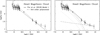 |
Fig. 3 Small Magellanic Cloud radio spectrum. The data points (dots) are from Table 4 of For et al. (2018). Left: preferred 1PL model 1 of For et al. (2018; solid line), and best-fitting third-order polynomial (dashed curve; see Table 4). Right: the two-component model (solid curve) that mimics the polynomial includes synchrotron radiation (dot-short-dashed curve) and thermal ff emission (dot-long-dashed curve); the primary and secondary synchrotron contributions are also shown (dashed, dotted curves). |
Summary of fits to the SMC radio spectrum.
4.2 LMC
Our fitting approach differs from that adopted for the SMC. The radio spectrum is best fit by a 2PL model interpreted as a combination of (individually 1PL) synchrotron and thermal ff components (For et al. 2018), which indicates that synchrotron emission is generated by a 1PL CRe spectrum. This is unlike the case of the SMC for which the interplay of primary and secondary CRe with different spectra results in a more structured, non-PL form. With the primary CRe spectrum determined from fitting the radio data, the Compton γ-ray yield is calculated.
To this a modeled pionic component is added and fit to the γ-ray data. Doing so enables the determination of the secondary CRe spectrum and the resulting yields, which turn out to be very minor in comparison with those of primary CRe; thus, no iteration of the fitting process is required.
The radio flux is dominated by synchrotron emission with α = 0.66 at the lowest measured frequencies, and by thermal ff emission with α = −0.1 at the highest frequencies (For et al. 2018). Adopting these spectral indices for the two components, we fit the full radio database with Te = 1.3 × 10⁴ K and F(Hα) = 2 × 10⁻⁷ erg cm−2 s−1 (Toribio San Cipriano et al. 2017; Kennicutt et al. 1995) for the thermal ff component, and B = 4.3 µG (Gaensler et al. 2005)5, Ne0 ≈ 3.5 × 10⁻⁷ cm−3 and γmax ≃ 2.4 × 10⁴ for the synchrotron. The cutoff is needed for consistency with the measured flux at ν ≳ 3 × 10²³ Hz. We should mention at this point that subsequent results (see below) suggest that the secondary CRe are only ~10% of the total. So the (quasi-) 1PL primaries dominate the CRe population (Fig. 2) and the emerging synchrotron emission. Therefore, the combined synchrotron and thermal ff radio spectrum matches the smooth 2PL profile of the For et al. (2018) fit. The radio model is shown in Fig. 5.
Next, we calculate the X-ray and γ-ray Compton and NT bremsstrahlung yields from (primary) CRe scattering off CMB-EBL-GFL photons and thermal plasma nuclei. To this end, we assume the photon fields described in Sect. 3 and, respectively, a plasma characterized by an average density ni = 0.012 cm−3 (Sasaki et al. 2002; Cox et al. 2006) and metallicity Z2 = 1.2 (Sasaki et al. 2002). Both emissions fall short of reproducing the γ-ray data.
The pionic emission is computed with nHI = 1 cm3 (from MHI = 3.8 × 10⁸M⊙; Staveley-Smith et al. 2003) and  = 6.6 × 10⁻² cm−3 (from
  = 5 × 10⁷M⊙, measured from CO emission; Fukui et al. 2008). From our fitting, the matching CRp spectrum has qp = 2.38 and
  = 80 GeV for the T+17 data (Fig. 6-top) and qp = 2.6 and
  = 25 GeV for the A+16 data (Fig. 6-bottom). The corresponding CRp energy densities are, respectively, 1 and 1.5 eV cm−3, the difference being largely due to the somewhat higher flux level in the A+16 data. In spite of the observational uncertainties in the two datasets, we see that for either dataset the pionic yield largely dominates the γ-ray emission, so the pionic nature of the measured γ-ray spectrum appears well established. In addition to the dominant pionic component a subdominant 7% (5%) leptonic contribution peaks at 500 (400) MeV, similarly to the pionic contribution: Comptonized COB and NT bremsstrahlung emissions contribute, respectively, 6.5% (4%) and 0.5% (1%) to the peak of the observed emission in the T+16 (A+16) database.
The secondary CRe spectrum is derived and fitted analytically, as described in Sect. 4.1; the fitting parameters are listed in Table 3 for both sets of LAT data. As mentioned, in both cases the radiative contribution of the secondary CRe is minor; this means that the corresponding primary PL spectra are essentially the same6, and (for each dataset) no fitting iteration is required. The primary and secondary CRe spectra are shown in Fig. 2.
Primary CRe largely dominate the CRe population in the LMC, even more so than in the SMC. However, their density is effectively unconstrained because it depends on assuming a magnetic field value (even though deduced from Faraday-rotation measurements, as in our case) rather than using a value derived by modeling the NT-X-ray emission as Comptonized CMB radiation (e.g., Persic & Rephaeli 2019a,b) or the hard X-ray-MeV emission (when it becomes available) as Comptonized IR radiation. Appreciable modeling uncertainty also stems from the inter-dependence among primary CRe parameters which results in a range of acceptable values of the spectral index and normalization, qe = 2.26 with Ne0 = 2.22 × 10⁻⁷ cm and γmax = 2.0 × 10⁴, as well as qe = 2.40 with Ne0 = 6.21 × 10⁻⁷ cm−3 and γmax = 2.7 × 10⁴ 7.
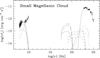 |
Fig. 4 Broadband (76 MHz–53.7 GeV) NT SED of the SMC disk. Data points (Table 1) are shown as dots, the model predictions as curves. Emission components are plotted by the following line types: synchrotron, dot-long-dashed; thermal ff, dot-short-dashed; total radio, solid; Comptonized CMB, long-dashed; Comptonized starlight (EBL+FGL), short-dashed; NT bremsstrahlung, dotted; pionic, solid. For each type of NT leptonic yield secondary, primary, and total emissions are denoted as curves of progressively higher flux. |
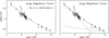 |
Fig. 5 Large Magellanic Cloud radio spectrum. The data points (dots) are from Table 2 of For et al. (2018). Left: model 3 of For et al. (2018, 2PL), shown as a solid curve. Right: the two-component model (solid curve) includes synchrotron radiation (dot-short-dashed curve) and thermal ff emission (dot-long-dashed curve); the dashed and dotted curves denote the primary and secondary synchrotron contributions, respectively (the latter corresponds to the T+17 γ-ray dataset). |
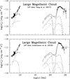 |
Fig. 6 Broadband (radio-γ, 19.7 MHz – 100 GeV) SED of the LMC disk. Data points (Table 2) are shown as dots: γ-ray data are from T+17 (top; reference set) and A+16 (bottom; auxiliary set). Model predictions are shown as curves. Emission components are plotted by the following line types: synchrotron, dot-long-dashed; thermal ff, dot-short-dashed; total radio, solid; Comptonized CMB, long-dashed; Comptonized starlight (EBL+FGL), short-dashed; NT bremsstrahlung, dotted; pionic, solid. For each type of NT leptonic yield secondary, primary, and total emissions are denoted as curves of progressively higher flux. In the X-ray and γ-ray range, on top of the emissions resulting from the various radiative processes a solid line indicates the cumulative emission. |
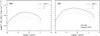 |
Fig. 7 Neutrino spectral emissions in the Magellanic Clouds. The LMC panel refers to the T+17 Fermi/LAT dataset. |
5 Neutrino emission
With an apparent dominant π0-decay origin of the γ rays produced in the interstellar medium of both MCs, it is clear that π± -decay neutrinos are also produced. Our calculations (following Kelner et al. 2006) of the predicted muon- and electron-neutrino spectra of the two galaxies indicate (Fig. 7) that the broadly peaked (~0.1–10 GeV) neutrino flux is too low for detection by current and upcoming v projects. This conclusion is based on the estimated observation time needed to detect the LMC with an experiment with detection sensitivity comparable to the Antarctica-based IceCube+DeepCore Observatory, the most sensitive current or planned v-detector at neutrino energies 10 < Ev/GeV < 100 (e.g., Bartos et al. 2013). The effective area of the observations (Abbasi et al. 2012) is Aeff(Ev) = cm2 (for vµ, two times smaller for ve) in this energy range (Bartos et al. 2013). Only in the narrow energy range 10–50 GeV do the IceCube+DeepCore sensitivity and the LMC predicted diffuse spectral v-flux effectively overlap (cf. the T+17 LAT dataset). In this band the LMC flux can be approximated as
  cm−2 s−1 GeV−1. The corresponding number of detected neutrinos,
  , is Nv ~ 10(tobs yr−1). The detector background (for up-going events) is dominated by atmospheric neutrinos produced by cosmic rays in the northern hemisphere; its energy spectrum is approximately flat in the relevant energy range, at a level ~102(dΩLMC/1.6sr) Gev−1 yr−1 (Bartos et al. 2013 and references therein). So the net 10–50 GeV background rate is ~4 × 10³(∆ΩLMC/1.6sr) yr−1 ~ 60 yrv1 assuming the LMC angular radius to be 5 deg). Based on this crude estimate, observation of diffuse GeV neutrinos from the LMC disk would imply S/N < 0.2.
6 Conclusion
The SMC and the LMC, star-forming Galactic satellite galaxies, are among the brightest sources in the Fermi/LAT γ-ray sky. We self-consistently modeled the radio-γ SED of both galaxies using the latest available radio and LAT data, using exact emissivity formulae for the relevant emission processes. Both SEDs were modeled with the radio data interpreted as a combination of NT electron synchrotron emission and thermal electron bremsstrahlung, and the γ-ray data as a combination of π0-decay emission from CRp interacting with the ambient gas plus leptonic emission. The CRp spectra appear similar in the two galaxies with qp ~ 2.4, and up ~ 1 eV cm−3. Our spectral findings are qualitatively and quantitatively new for the SMC, and confirm and strengthen previous results for the LMC. In detail, we quantified the (Lopez et al. 2018) suggestion of a mostly pionic origin of the LAT-measured γ-ray emission of the SMC, only ≲3% of the peak flux being by NT bremsstrahlung; for the LMC, our analysis suggests that 93%, 6.5%, and 0.5% of the LMC peak γ-ray flux (at 0.5 GeV) are accounted for by pionic, Comptonized starlight, and NT-bremsstrahlung emission, in broad agreement with Foreman et al. (2015). As we have noted, for the SMC disk we used the (Lopez et al. 2018) LAT dataset which is only mildly contaminated by an estimated ~ 10% contribution from unresolved pulsars, whereas for the LMC disk we used LAT datasets based on maps that do not include emission from local gas and CR inhomogeneities associated with actively star-forming regions (A+16; T+17). Thus, our pionic emission modeling results are unlikely to be appreciably affected by emission from individual sources.
As stated in Sect. 4, our treatment is based on determining the particle steady-state spectral distributions in the disk by fits to the radio and γ-ray data, using previously deduced mean disk values of the gas density, magnetic and radiation fields. An assessment of the combined uncertainties in the predicted particle radiative (and neutrino) yields is based first on the precision level of the observationally determined values of ng and B. Although the deduced CRe normalization is (essentially) independent of ng, its dependence on B is significant, Ne0 ∝ B−(α+1), which is roughly B−1.7. The deduced CRp normalization is Np0 ∝ 1/ng. Given the substantial uncertainties in both ng and B, it is clear that these also impact the overall normalization of the particle spectra, which can be uncertain by a factor of 2–3. However, the constraining power of the fits to the measurements is mostly in the well-known spectral shapes of the predicted synchrotron and π0-decay processes. As explained in the previous section, the spectral fits are quite good, with an average level of statistical uncertainty of ~20% on the primary CRe spectral parameters. Even though substantial, the overall level of uncertainty is not large enough to question our qualitative conclusion on the pionic nature of the γ-ray emission.
The SMC radio data have large error bars below 230 MHz where qe would be best determined, are unsampled (but for one point) between 230 and 1400 MHz where the effect of the spectral truncation would be observed, and are only sparsely sampled above 1400 MHz. This leaves both qe and γmax poorly determined. The LMC radio spectral data permit determination only of qe as no truncation is apparent; we estimated γmax by estimating its lower limit implied by the radio spectrum and its upper limit implied by the γ spectrum. A larger value would shift the Comptonized starlight (EBL+FGL) blue peak to higher frequencies and to a higher flux level, deteriorating the fit to the γ spectrum at frequencies log(v) > 24. Our joint analysis of the broadband SED of the MCs using exact emissivity formulae, and the leptonic radio and γ emissions are coupled and are based on independent measures (independent of particle-field energy equipartition considerations) of the magnetic field, so the pionic emission is formally determined by modeling the residuals of the LAT data after the leptonic yield is accounted for. In general, uncertainties on the CRe spectrum affect the determination of the CRp spectrum because the latter is obtained by fitting the γ data once the leptonic yields have been properly accounted for. However, we feel our CRp results here are reasonably solid because of the clear dominance of pionic emission in the γ spectrum.
For the SMC the LAT data are sufficient to define the CRp spectral parameters, qp = 2.4 and  = 30 GeV. For the LMC, however, some inconsistency between the T+17 and A+16 LAT datasets implies the derived CRp spectrum to be, respectively, flatter (qp = 2.4) with no clearly discernible high-energy truncation
  and steeper (qp = 2.6) with a clear truncation (
 = 25 GeV) and a ~50% higher normalization. Both qp values are consistent within the errors with the Foreman et al. (2015) earlier estimate. The reason for the discrepancy between the two datasets is not obvious, as the T+17 and A+16 data extraction regions largely overlap with each other and with the LMC disk, and both have been cleaned for identified sources (point-like or extended). It should be noted that in the T+17 dataset the quality of the four highest-frequency points does not allow a definite estimate of
  , whereas the four lowest-frequency points enable a clear view of the rising portion of the pionic hump. Ongoing Fermi/LAT measurements would likely improve the quality of the spectrum and clarify this issue. For both galaxies we obtained truncation energies systematically higher for CRp than for CRe, probably because energy losses are much less efficient for the former than for the latter in the relatively low-density MC interstellar gas.
The secondary CRe spectra are, at best, as well determined as those of the parent CRp. Our model secondary spectra (with no free parameters) are relatively well defined in the MCs. However, the primary CRe spectra, determined by fitting radio data after secondary CRe are accounted for, are less well constrained. First, the measured radio fluxes include emission from individual background and MC-disk point sources that contribute ~20% of the total emission and are spectrally similar to the overall emission (For et al. 2018), so there is some intrinsic uncertainty in the predicted extended emission’s spectral shape and normalization (Ne0 is biased high). Secondly, because of the qe-Ne0 degeneracy the uncertainty on Ne0 affects the determination of the spectral slope. Thus, primary CRe are rather poorly constrained in both MCs. In spite of this, our assumption of a (truncated) 1PL representing primary CRe is sound. The PL is a fair approximation, over the relevant CRe energy range, of the actual spectrum computed accounting for realistic energy losses in the MC disk environments. The approximation is particularly good for the LMC.
A possible underestimate of the gas content in the MC due to the presence of dark (unseen) neutral gas (i.e., HI gas) optically thick in the 21 cm line and/or H2 gas with no associated CO emission, could increase the uncertainty on the total (atomic and molecular) gas density. The CO (J = 1–0) transition, often used to detect the total H2 mass, may be hard to detect in low-Z galaxies such as the MC (Rolleston et al. 2002; Requena-Torres et al. 2016), so the relatively bright [C II]λ158 µm line can be used instead: indeed, >70% of the total H2 mass may not have been traced by CO (1-0) in dwarf galaxies, but is well traced by [CII]λ158 µm (Madden et al. 2020). Another important aspect to investigate is the mixing of dust into the interstellar medium (ISM) and the spatial variations of their properties (gas clumpiness affects emission levels, see above). Comparing the distributions of the IR dust emission and several gas tracers (Hα, 21 cm, CO emission), their different emission processes highlight the distribution of gas under different conditions. In the LMC this analysis reveals that (i) dust emission, sampled in the Multiband Imaging Photometer for Spitzer (MIPS) 70 and 160 µm bands, is well mixed with the large-scale HI 21 cm emission; (ii) Hα from star-forming HII regions is confined to the massive star formation region where also warmer (~ 120 K) 24 µm emission is found; and (iii) the Spitzer InfraRed Array Camera (IRAC) 8 µm band that traces polycyclic aromatic hydrocarbons correlates well with the HI gas, but is absent from the massive star-forming HII regions. All in all, the dust emission revealed by the combined IRAC 8 µm and MIPS 24, 70, and 160 µm bands traces all three phases of the ISM gas (Meixner et al. 2006). Underestimating the gas content would affect the particle spectra in the following ways: (i) overestimating the CRp spectral normalization; (ii) underestimating the Coulomb and bremsstrahlung energy losses, b0(γ) and b1(γ), (Rephaeli & Persic 2015), which would cause the computed steady-state secondary CRe spectrum to be, respectively, higher and steeper; (iii) biasing the derived primary CRe spectrum lower and flatter.
Uncertainties in the 3D structure of the MCs (mainly for the SMC; Abdo et al. 2010b) directly affect only the CRe and CRp spectral normalizations, to match the spectral flux when the emitting volume changes; this holds for the relevant leptonic emissivities, which depend linearly on the CRe normalization. Thus, model SEDs are nearly unaffected by variations of the MC structure parameters. Another source of uncertainty in Ne0 stems from assuming a magnetic field (for both galaxies), in our case field values derived by Faraday rotation studies of extra-galactic polarized sources seen through the MCs. These field strengths are measured along the line of sight to the background sources; thus, they are line-averaged fields, whereas the field in the synchrotron emissivity expression is a volume average. The two values may or may not be the same; the potential mismatch introduces another systematic uncertainty in the determination of Ne0 from fitting the radio spectrum. For example, in principle, if B is biased high, Ne0 and all leptonic yields are biased low, so the resulting Np0 is biased high.
The main breakthrough needed in MC SED studies is the measurement of diffuse NT X-ray emission from their disks. As exemplified in our studies of radio-lobe SEDs (Persic & Rephaeli 2019a,b), the NT 1 keV flux, interpreted as Comptonized CMB emission, sets the normalization of the CRe spectrum. In the MC case, given that the excellent pionic fit to the γ-ray emission firmly defines the secondary spectrum, the 1 keV flux would effectively measure the primary normalization. Modeling the radio spectrum as synchrotron radiation would then provide the primary spectral shape and, importantly, the magnetic field. A spectral determination of B would bypass the need to assume particle-field equipartition, and would return a volume-averaged value better representing the mean field than the line averages yielded by Faraday rotation-based measurements. Deeper X-ray observations of both MCs, with better spatial and spectral resolution than currently available will be highly beneficial to searching the diffuse disk emission for a NT component.
Acknowledgement
We acknowledge insightful comments by an anonymous referee that improved clarity and presentation of our work.
References
- Abbasi, R., Abdou, Y., Abu Zayyad, T., et al. 2012, Astropart. Phys., 35, 615 [NASA ADS] [CrossRef] [Google Scholar]
- Abdo, A. A., Ackermann, M., Ajello, M., et al. 2010a, A&A, 512, A7 [NASA ADS] [CrossRef] [EDP Sciences] [Google Scholar]
- Abdo, A. A., Ackermann, M., Ajello, M., et al. 2010b, A&A, 523, A46 [NASA ADS] [CrossRef] [EDP Sciences] [Google Scholar]
- Ackermann, M., Albert, A., Atwood, W. B., et al. 2016, A&A, 586, A71 [NASA ADS] [CrossRef] [EDP Sciences] [Google Scholar]
- Alvarez, H., Aparici, J., & May, J. 1987, A&A, 176, 25 [NASA ADS] [Google Scholar]
- Bartos, I., Beloborodov, A. M., Hurley, K., & Márka, S. 2013, Phys. Rev. Lett., 110, 241101 [NASA ADS] [CrossRef] [Google Scholar]
- Blumenthal, G. R., & Gould, R. J. 1970, RvMP, 42, 237 [NASA ADS] [Google Scholar]
- Condon, J. J. 1992, ARAA, 30, 575 [NASA ADS] [CrossRef] [Google Scholar]
- Cooray, A. 2016, R. Soc. Open Sci., 3, 150555 [NASA ADS] [CrossRef] [Google Scholar]
- Cox, N. L. J., Cordiner, M. A., Cami, J., et al. 2006, A&A, 447, 991 [NASA ADS] [CrossRef] [EDP Sciences] [Google Scholar]
- For, B.-Q., Staveley-Smith, L., Hurley-Walker, N., et al. 2018, MNRAS, 480, 2743 [NASA ADS] [CrossRef] [Google Scholar]
- Foreman, G., Chu, Y. H., Gruendl, L., et al. 2015, ApJ, 808:44 [NASA ADS] [CrossRef] [Google Scholar]
- Franceschini, A., & Rodighiero, G. 2017, A&A, 603, A34; Erratum: 2018, 614, C1 [NASA ADS] [CrossRef] [EDP Sciences] [Google Scholar]
- Fukui, Y., Kawamura, K., Minamidami, T., et al. 2008, ApJS, 178, 56 [NASA ADS] [CrossRef] [Google Scholar]
- Gaensler, B. M., Haverkorn, M., Staveley-Smith, L., et al. 2005, Science, 307, 1610 [NASA ADS] [CrossRef] [Google Scholar]
- Haynes, R. F., Klein, U., Wayte, S. R., et al. 1991, A&A, 252, 475 [NASA ADS] [Google Scholar]
- Kelner, S. R. et al., 2006, Phys. Rev. D, 74, 034018; Erratum: 2009, 79, 039901(E) [NASA ADS] [CrossRef] [Google Scholar]
- Kennicutt, R. J.Jr., Bresolin, F., Bomans, D.J., Bothun, G.D., & Thompson, I.B. 1995, AJ, 109, 594 [NASA ADS] [CrossRef] [Google Scholar]
- Leroy A., Bolatto A., Stanimirovic S., Mizuno N., Israel F., Bot C., 2007, ApJ, 658, 1027 [NASA ADS] [CrossRef] [Google Scholar]
- Klein, U., Wielebinski, R., Haynes, R. F., & Malin, D. F. 1989, A&A, 211, 280 [NASA ADS] [Google Scholar]
- Loiseau, N., Klein, U., Greybe, A., Wielebinski, R., & Haynes, R. F. 1987, A&A, 178, 62 [NASA ADS] [Google Scholar]
- Lopez, L. A., Auchettl, K., Linden, T., et al. 2018, ApJ, 867, 44 [NASA ADS] [CrossRef] [Google Scholar]
- Madden, S. C., Cormier, D., Hony, S., et al. 2020, A&A, 643, A141 [NASA ADS] [CrossRef] [EDP Sciences] [Google Scholar]
- Mao, S. A., Gaensler, B. M., Stanimirovic, S., et al. 2008, ApJ, 688, 1029 [NASA ADS] [CrossRef] [Google Scholar]
- Mao, S. A., McClure-Griffiths, N. M., Gaensler, B. M., et al. 2012, ApJ, 759, 25 [NASA ADS] [CrossRef] [Google Scholar]
- Meixner, M., Gordon, K. D., Indebetouw, R., et al. 2006, ApJS, 132, 2268 [CrossRef] [Google Scholar]
- Mills, B. Y. 1955, Aust. J. Phys., 8, 368 [NASA ADS] [CrossRef] [Google Scholar]
- Mills, B. Y. 1959, Handbuch Physik, 53, 239 [NASA ADS] [Google Scholar]
- Mountfort, P. I., Jonas, J. L., De Jager, G., & Baart, E. E. 1987, MNRAS, 226, 917 [NASA ADS] [CrossRef] [Google Scholar]
- Nishiuchi, M., Imanishi, K., Tsujimoto, M., Yokogawa, J., & Koyama, K. 1999, in Star Formation 1999, eds. T. Nakamoto, Nobeyama Radio Observatory, 54 [Google Scholar]
- Nishiuchi, M., Yokogawa, J., & Koyama, K. 2001, in New Century of X-ray Astronomy, ASP Conference Series, 251, eds. H. Inoue, & H. Kunieda, 264 [Google Scholar]
- Persic, M., & Rephaeli, Y. 2019a, MNRAS, 485, 2001; Erratum: 2019, 486, 950 [NASA ADS] [CrossRef] [Google Scholar]
- Persic, M., & Rephaeli, Y. 2019b, MNRAS, 490, 1489 [NASA ADS] [CrossRef] [Google Scholar]
- Points, S. D., Chu, Y. H., Snowden, S. K., & Smith, R. C. 2001, ApJS, 136, 99 [NASA ADS] [CrossRef] [Google Scholar]
- Rephaeli, Y., & Persic, M. 2015, ApJ, 805, 111 [NASA ADS] [CrossRef] [Google Scholar]
- Rephaeli, Y., & Sadeh, S. 2019, MNRAS, 486, 2496 [NASA ADS] [CrossRef] [Google Scholar]
- Requena-Torres, M. A., Israel, F. P., Okada, Y., et al. 2016, A&A, 589, A28 [NASA ADS] [CrossRef] [EDP Sciences] [Google Scholar]
- Rolleston, W. R. J., Trundle, C., & Dufton, P. L. 2002, A&A, 396, 53 [NASA ADS] [CrossRef] [EDP Sciences] [Google Scholar]
- Sasaki, M., Haberl, F., & Pietsch, W. 2002, A&A, 392, 103 [NASA ADS] [CrossRef] [EDP Sciences] [Google Scholar]
- Shain, C. A. 1959, in IAU Symp. 9, Observations of Extragalactic Radio Emission, ed. R.N. Bracewell (Stanford, CA: Stanford University Press), 328 [Google Scholar]
- Spitzer, L.Jr., 1978, Physical Processes in the Interstellar Medium (Wiley) [Google Scholar]
- Sreekumar, P., Bertsch, D. L., Dingus, B. L., et al. 1992, ApJ, 400, L67 [NASA ADS] [CrossRef] [Google Scholar]
- Stanimirović, S., Staveley-Smith, L., Dickey, J. M., Sault, R. J., & Snowden S.L. 1999, MNRAS, 302, 417 [CrossRef] [Google Scholar]
- Staveley-Smith, L., Kim, S., Calabretta, M. R., Haynes, R. F., & Kesteven, M. J., 2003, MNRAS, 339, 87 [NASA ADS] [CrossRef] [Google Scholar]
- Tang, Q. W., Peng, F. K., Liu, R. Y., Tam, P. H. T., & Wang X.Y. 2017, ApJ, 843, 42 [NASA ADS] [CrossRef] [Google Scholar]
- Toribio San Cipriano, L., Domínguez-Guzmán, G., Esteban, C., et al. 2017, MNRAS, 467, 3759 [NASA ADS] [CrossRef] [Google Scholar]
- Wang, Q., Hamilton, T., Helfand, D. J., & Wu, X. 1991, ApJ, 374, 475 [NASA ADS] [CrossRef] [Google Scholar]
Emission components are labeled “E” in Ackermann et al. (2016) and “G” in Tang et al. (2017).
As to the prominent 30 Dor massive star-forming region, Ackermann et al. (2016) emphasize that it shines inGeV γ rays mainly because of the presence of PSR J0540-6919 and PSR J0537-6910.
Denoting the total cross-section for inelastic pp collisions σpp(Ep) (see Eq. (79) in Kelner et al. 2006), the secondary CRe injection spectrum is QSe(γ) = (8/3) me  ng Np0
 ![${N_{{\rm{p0}}}}{\left[ {{m_{\rm{p}}} + \left( {4{m_{\rm{e}}}/{\kappa _{{\pi ^ \pm }}}} \right)\gamma } \right]^{ - {q_{\rm{p}}}}}{\sigma _{{\rm{pp}}}}\left( {{m_{\rm{p}}} + {E_{{\pi ^ \pm }}}/{k_{{\pi ^ \pm }}}} \right)$](/articles/aa/full_html/2022/10/aa43391-22/aa43391-22-eq36.png) for
for  , with
  and
and  . The corresponding steady-state distribution is
  , where b(γ) is the radiative energy loss term. In a magnetized medium consisting of ionized, neutral, and molecular gas, it is
  where bj(γ) are loss terms appropriate to each gas phase (see Eqs. (4)–(6) of Rephaeli & Persic 2015). Nse(γ) is analytically approximated by
 ![$N_{{\rm{se}}}^{{\rm{fit}}}\left( \gamma \right) = {N_{{\rm{se,0}}}}{\gamma ^{ - {q_1}}}{\left( {1 + \gamma /{\gamma _{b1}}} \right)^{{q_1} - {q_2}}}\exp \left[ { - {{\left( {\gamma /{\gamma _{b2}}} \right)}^\eta }} \right]$](/articles/aa/full_html/2022/10/aa43391-22/aa43391-22-eq42.png) , where q1, q2 and γb1, γb2 are the low- and high-energy spectral indices and breaks; η gauges the steepness of the high-end cutoff.
, where q1, q2 and γb1, γb2 are the low- and high-energy spectral indices and breaks; η gauges the steepness of the high-end cutoff.
This field value, from a Faraday rotation study of the LMC, is consistent with the Mao et al. (2012) estimates, Beq ~ 2 µG, from equipartition with CRp assuming qp = 2 and B < 7 µG from using a (deduced) lower limit on Ne0 in fitting the 1.4 GHz radio flux.
All Tables
All Figures
|
Fig. 1 Gamma-ray spectra in the Magellanic Clouds. Curves represent: (top) pionic emission, solid; (middle and bottom, in decreasing flux): total gamma and pionic emissions, solid, and total and primary NT bremsstrahlung, dashed. |
| In the text | |
|
Fig. 2 CRe spectra in the Magellanic Clouds. The curves are the secondary spectra (dashed), primary spectra (dotted), and the primaries’ local PL representations (solid). In each panel the normalization of the primary CRe spectrum to its PL counterpart is chosen such that they nearly overlap. The primary CRe injection indices, qi, are 2.28 (SMC) and 2.23 (LMC). The two LMC CRe spectra panels refer, respectively, to the T+17 and A+16 Fermi/LAT datasets, as secondary spectra are derived from the pionic fits to the γ-ray data. |
| In the text | |
|
Fig. 3 Small Magellanic Cloud radio spectrum. The data points (dots) are from Table 4 of For et al. (2018). Left: preferred 1PL model 1 of For et al. (2018; solid line), and best-fitting third-order polynomial (dashed curve; see Table 4). Right: the two-component model (solid curve) that mimics the polynomial includes synchrotron radiation (dot-short-dashed curve) and thermal ff emission (dot-long-dashed curve); the primary and secondary synchrotron contributions are also shown (dashed, dotted curves). |
| In the text | |
|
Fig. 4 Broadband (76 MHz–53.7 GeV) NT SED of the SMC disk. Data points (Table 1) are shown as dots, the model predictions as curves. Emission components are plotted by the following line types: synchrotron, dot-long-dashed; thermal ff, dot-short-dashed; total radio, solid; Comptonized CMB, long-dashed; Comptonized starlight (EBL+FGL), short-dashed; NT bremsstrahlung, dotted; pionic, solid. For each type of NT leptonic yield secondary, primary, and total emissions are denoted as curves of progressively higher flux. |
| In the text | |
|
Fig. 5 Large Magellanic Cloud radio spectrum. The data points (dots) are from Table 2 of For et al. (2018). Left: model 3 of For et al. (2018, 2PL), shown as a solid curve. Right: the two-component model (solid curve) includes synchrotron radiation (dot-short-dashed curve) and thermal ff emission (dot-long-dashed curve); the dashed and dotted curves denote the primary and secondary synchrotron contributions, respectively (the latter corresponds to the T+17 γ-ray dataset). |
| In the text | |
|
Fig. 6 Broadband (radio-γ, 19.7 MHz – 100 GeV) SED of the LMC disk. Data points (Table 2) are shown as dots: γ-ray data are from T+17 (top; reference set) and A+16 (bottom; auxiliary set). Model predictions are shown as curves. Emission components are plotted by the following line types: synchrotron, dot-long-dashed; thermal ff, dot-short-dashed; total radio, solid; Comptonized CMB, long-dashed; Comptonized starlight (EBL+FGL), short-dashed; NT bremsstrahlung, dotted; pionic, solid. For each type of NT leptonic yield secondary, primary, and total emissions are denoted as curves of progressively higher flux. In the X-ray and γ-ray range, on top of the emissions resulting from the various radiative processes a solid line indicates the cumulative emission. |
| In the text | |
|
Fig. 7 Neutrino spectral emissions in the Magellanic Clouds. The LMC panel refers to the T+17 Fermi/LAT dataset. |
| In the text | |
Current usage metrics show cumulative count of Article Views (full-text article views including HTML views, PDF and ePub downloads, according to the available data) and Abstracts Views on Vision4Press platform.
Data correspond to usage on the plateform after 2015. The current usage metrics is available 48-96 hours after online publication and is updated daily on week days.
Initial download of the metrics may take a while.