| Issue |
A&A
Volume 685, May 2024
|
|
|---|---|---|
| Article Number | A7 | |
| Number of page(s) | 18 | |
| Section | Cosmology (including clusters of galaxies) | |
| DOI | https://doi.org/10.1051/0004-6361/202347918 | |
| Published online | 30 April 2024 | |
Simulations of early structure formation: Properties of halos that host primordial star formation⋆
Univ Lyon, Ens de Lyon, Univ Lyon1, CNRS, Centre de Recherche Astrophysique de Lyon UMR5574, 69007 Lyon, France
e-mail: This email address is being protected from spambots. You need JavaScript enabled to view it.
Received:
8
September
2023
Accepted:
8
January
2024
Abstract
Context. Population III (pop III) stars were born in halos characterised by a pristine gas composition. In such a halo, once the gas density reaches nH ∼ 1 cm−3, molecular cooling leads to the collapse of the gas and the birth of pop III stars. Halo properties, such as the chemical abundances, mass, and angular momentum can affect the collapse of the gas, thereby leading to the pop III initial mass function (IMF) of star formation.
Aims. We want to study the properties of primordial halos and how halos that host early star formation differ from other types of halos. The aim of this study is to obtain a representative population of halos at a given redshift hosting a cold and massive gas cloud that enables the birth of the first stars.
Methods. We investigated the growth of primordial halos in a ΛCDM Universe in a large cosmological simulation. We used the hydrodynamic code RAMSES and the chemical solver KROME to study halo formation with non-equilibrium thermochemistry. We then identified structures in the dark and baryonic matter fields, thereby linking the presence or absence of dense gas clouds to the mass and the physical properties of the hosting halos.
Results. In our simulations, the mass threshold for a halo for hosting a cold dense gas cloud is ≃7 × 10⁵ M⊙ and the threshold in the H2 mass fraction is found to be ≃2 × 10⁻⁴. This is in agreement with previous works. We find that the halo history and accretion rate play a minor role. Here, we present halos with higher HD abundances, which are shown to be colder, as the temperature in the range between 102 − 104 cm−3 depends on the HD abundance to a large extent. The higher fraction of HD is linked to the higher spin parameter that is seen for the dense gas.
Key words: stars: Population II / stars: Population III / Galaxy: formation / early Universe / dark ages / reionization / first stars
The code used in the paper is available at https://github.com/Lenoble-lab/ramses-krome
© The Authors 2024
 Open Access article, published by EDP Sciences, under the terms of the Creative Commons Attribution License (https://creativecommons.org/licenses/by/4.0), which permits unrestricted use, distribution, and reproduction in any medium, provided the original work is properly cited.
This article is published in open access under the Subscribe to Open model. This email address is being protected from spambots. You need JavaScript enabled to view it. to support open access publication.
1. Introduction
The formation of the first stars is a critical chapter in cosmic history, marking the end of the cosmic dark ages and the dawn of the first luminous objects. Primordial stars, born from pristine gas before the onset of metal enrichment, were likely to be much more massive and short-lived than their modern counterparts, thereby influencing the subsequent evolution of the Cosmos (Hirano et al. 2014). The precise knowledge of their characteristic mass or the primordial initial mass function (IMF) is of primary importance to constrain the global evolution of the Universe and it largely remains an open question (Stacy et al. 2016).
At early time, the Universe was nearly homogenous. Observations of the cosmic microwave background (CMB) have shown fluctuations of one part in 105. These small-amplitude fluctuations grew due to gravitational instability into the first bounded objects and then into present-days galaxies. Overall, this evolution is aptly predicted by the ΛCDM model, which requires the presence of dark matter (DM). In this model, the initial primordial power-law spectrum is modified over time as a result of perturbation growth. The DM first starts to collapse and to form the first bounded objects that can accrete gas.
To collapse into stars, the baryonic gas needs to radiate away the gravitational binding energy released during the collapse. It is thus a competition between the timescales for cooling and freefall. The classic criterion from Rees & Ostriker (1977) states that if tcool ≤ tff, the gas will collapse. In pristine gas, the only available coolants are molecular hydrogen (H2) and (to a lesser extent) the HD molecule. From the equality in the two timescales, a threshold in the H2 fraction can be derived. With this simple theoretical framework, Tegmark et al. (1997) found that population III (pop III) stars were born in the first massive bound objects of ≃106 M⊙ at z ≃ 20 − 30. Today, this is still the overall framework according to recent 3D hydrodynamic simulations which follow the growth of mini-halos with masses of 105 − 106 M⊙ in the early Universe until the formation of a collapsing cold gas clump (Yoshida et al. 2003; Hirano et al. 2015). Higher resolutions simulations using the zoom-in technique can even link the formation of halos at large scales to the birth of protostars, thereby estimating the primordial IMF (Hirano et al. 2014; Stacy et al. 2016).
However, it has been shown that the properties of the host halo have a large impact on the enclosed star formation (Bromm et al. 2002; Hirano et al. 2014; McKee & Tan 2008). The angular momentum, shape, and accretion rate of a halo (among other properties) can influence the collapse and the results from a zoom-in simulation depend a great deal on the properties of the chosen halo. Hence, it is important to study which halos lead to primordial star formation. Previous works have already pointed out this need for statistical studies. de Souza et al. (2013) ran cosmological simulations to link the presence of a star-forming clouds with halo properties. Hirano et al. (2015) performed a set of cosmological simulations to derive the primordial IMF. They identified distinct populations of primordial stars, noting whether they were formed with or without a far-ultraviolet background radiation (due to the presence of nearby stars). To determine the IMF of the first stars in absence of any radiation, they used the correlation between the accretion rate at the jeans scale and the final stellar mass found in their first paper (Hirano et al. 2014).
Halo-scale angular momentum is one of the key factors determining subsequent collapse on the scale of star formation, in particular, fragmentation and disk formation. McKee & Tan (2008) studied how the accretion rate depends on the angular momentum. They concluded that the primordial IMF is set by the distribution of entropy and the specific angular momentum of the accreting gas. Similarly, simulations from Bromm et al. (2002) have shown that the initial angular momentum favors a disk-like structure that may even fragment. However, the relation between the angular momentum of the parent DM halo and that of the dense gas is not obvious. The baryonic gas is bounded in the gravitational potential of the parent halo. As it is falling, its angular momentum may align to that of the parent halo. Hirano et al. (2015) found a weak correlation between the direction of the two angular momenta, which varies with redshift. Hence, the study the of distribution of angular momentum in primordial halos is clearly valuable. It is also a key factor in galaxy formation and the halo mass function itself. Druschke et al. (2018) ran high-resolution DM-only 3D simulations of primordial halo formation to study its distribution and correlation with larger-scale properties.
The shapes of halos can also have an impact (Pon et al. 2012). When the first stars form, halos are far from being spheroids and, instead, closer to ellipsoids, with three principal axes of different lengths. Again, Druschke et al. (2018) studied the distribution of the halo shape of halos in a DM-only 3D simulation. Kazantzidis et al. (2004), albeit their study was carried out at much lower redshifts (z = 1 − 2), showing that baryon physics have an important back-reaction on the DM distribution: taking gas cooling into account tends to change the shape of halos dramatically, making them more spherical compared to adiabatic ones. Thus, the modelling of detailed physical processes of the gas is necessary.
The most important process for primordial star formation is molecular formation and the path that leads to H2 cooling. The large-scale physical properties of a halo can have an impact on the chemical state of the dense gas. First, there seems to be a broad consensus on the existence of a threshold in H2 mass fraction at the halo scale above which a halo can host a cold collapsing gas cloud. Both theoretical works (Tegmark et al. 1997) and numerical simulations (Yoshida et al. 2003) pointed at a threshold of xH2 = 10−4 − 10−3 at the halo scale. However, it is not clear how the physical properties of the halo, in particular, the accretion rate or the angular momentum, could alter this value or trigger molecule formation. Then, at a higher density, when the central density peak reaches 107 cm−3, Hirano et al. (2015) found a link between the accretion rate at the virial scale and at the Jeans length of the star-forming region.
The role of HD cooling is debated. McGreer & Bryan (2008) studied the importance of HD formation and cooling with numerical simulations. They showed that HD cooling can be important within a halo if part of the gas is at a low temperature and a sufficiently high density to form HD preferentially over H2. They also observed that a high ionisation fraction can lead to HD formation and cooling until the CMB floor. This is also what has been observed by Hirano et al. (2015): some of their halos have a much higher HD fraction, which further cools down the gas. The properties leading to a higher HD fraction are still not clear. The H2 and HD abundances of the first structures depend on many factors in 3D hydrodynamic simulations, including the initial conditions of the halo, the assumed chemical network and various non-linear feedback loops (Klessen & Glover 2023).
The aim of this paper is to study the properties of the first primordial star-forming halos, using a large simulation with an updated chemical network that includes HD formation. Using our simulations, we determine how halos that host collapsing gas clouds and, hence, star formation are different from other non-star-forming halos; we also consider how the properties of these star-forming halos are distributed. To do this, our simulation needs to resolve the gas, from the large-scale structure in a cosmological volume to higher density, where the gas is collapsing, until star formation occurs. We can then identify star-forming halos and get a statistically representative population of low-mass halos at high redshift. This representative catalogue of halos can be use for future studies using the zoom-in technique.
The outline of this paper is as follows. First, in Sect. 2, we describe the numerical methodology of the hydrodynamic simulation and for the analysis and the initial conditions we use. Then, in Sect. 3, we present our results. Finally, Sect. 4 contains a discussion, followed by our conclusions in Sect. 5.
2. Methodology and numerical set-up
2.1. Numerical methodology
We used the adaptive mesh refinement (AMR) code RAMSES (Teyssier 2002) to solve the interaction of DM and hydrodynamics on a 3D adaptively refined mesh. For the hydrodynamics, we used the HLLC Riemann solver (Toro et al. 1994) and the MinMod slope limiter to construct gas variables at cell interfaces from their cell-centred values. To compute the gas equation of state, we used the constant adiabatic index γ = 5/3, which corresponds to an ideal monoatomic gas. This approximation is valid as the molecular fraction remains extremly low in the density range of this simulation (at most 10−3). We used the multigrid gravity solver implemented in RAMSES (Guillet & Teyssier 2011) and cloud-in-cell interpolation for DM particles.
The RAMSES code uses a cubical octree structure. The cell width at the refinement level ℓ is Δxℓ = 0.5ℓLbox, where Lbox is the width of the box. In our simulations, a cell is refined into eight equally sized children cells if either one of these two conditions is satisfied:
(a)  , where mDM is the mass of a DM particle, MDM, cell and Mbaryon, cell are the total DM and baryonic masses in the cell;
(b) the Jeans length is smaller than four cell widths, namely: if  , where
  with G the gravitational constant, ρ the gas density,
  is the sound speed of the gas, with T as the gas temperature, kB the Boltzmann constant, and mp the proton mass.
2.2. Initial conditions
We generated the cosmological initial conditions corresponding to a ΛCDM Universe with MUSIC (Hahn & Abel 2011) and the parameters as published by the Planck 2020 collaboration (Planck Collaboration VI 2020): Ωm = 0.3111, ΩΛ = 0.6889, Ωb = 0.04897, σ8 = 0.825, H0 = 67.66 km s−1 Mpc−1. Our fiducial simulation volume has a width of 1 cMpc/h and 5123 particles (corresponding to a minimum (coarse) level of 9). The coarse cell size is 1.9 ckpc/h (150 pc at z = 18) and reaches a maximum refinement level of 19 at the last snapshot at z = 18, corresponding to 0.14 pc. The DM is modelled by 5123 particles with mass mDM = 813 M⊙.
To test the resolution convergence of this simulation, we also ran a second simulation with half the box length and the same refinement levels and number of DM particles of 5123. In this simulation, mDM = 102 M⊙. It also reaches a maximum refinement level of 19 at z = 18. The parameters of the two simulations are shown in Table 1. We discuss of the choice of the box size and the resolution in the Sect. 3.1.
Simulation volumes used in this work.
We assumed the initial chemical abundances to be uniform in the whole volume at z = 100 when we started the simulation. We computed the chemical abundances at z = 100 with a one-zone model that takes into account the physical evolution of the Universe from z = 104. The model details are shown in Appendix B and the initial chemical abundances are summarised in Table 2.
Chemical abundances at z = 100.
2.3. Chemistry and cooling
We used the KROME code (Grassi et al. 2014) to resolve the chemistry. For each cell of RAMSES, the non-equilibrium chemistry is computed on-the-fly in each gas cell. The system of ordinary differential equations (ODEs) describing our chemical network is solved with the DLSODE solver (Byrne & Hindmarsh 1987), which generates the sparsity structure and the Jacobian of the system.
2.3.1. Chemical network
We used an updated chemical network consisting of 11 species: (e−, H, H+, H−, D, D+, He, H2,  , HD, and HeH+) and 23 reactions. All reactions can be found in Appendix C. The minimal network of Galli & Palla (1998) for H, D, and He has been updated from a comprehensive literature survey and new rate coefficients have been adopted for all 21 reactions (all reactions except H11 and H12). Simple modified-Arrhenius fits were found to adequately reproduce the literature data in the temperature range of 10–10 000 K. While differences in the fits of Galli & Palla (1998) do not generally exceed the investigated temperature range by more than a factor of 2–3, large deviations (up to a factor of 20) were observed for the formation and destruction reactions of HeH+. Full details (including the fitting coefficients) of the network will be described in Faure et al. (in prep.), but they are also available upon request.
For the three-body recombination of hydrogen (3H → H2 + H), the theoretical rate coefficient of Forrey (2013) was fitted with a modified-Arrhenius form. The Saha equation was then used to derive (and fit) the rate coefficient for the reverse reaction (Faure priv. comm.).
2.3.2. Molecule formation
Our chemical network is quite exhaustive, we describe here the main way in which H2 is formed and destroyed. In the physical conditions of our simulations, the main formation pathway for H2 is via the H− channel. In this process, electrons act as catalysts:
 (1)
(1)
 (2)
(2)
The two reactions are instantaneous as soon as one H− is formed. The other channel for H2 formation in the low-density regime is the  channel, but it is only dominant at very high redshifts (z > 200), where H− is easily destroyed by CMB photons (Galli & Palla 2013, by a factor ∼100 at 1000 K). The three-body reaction is dominant only at really high density (nH > 108 cm−3) and quickly converts the gas into fully molecular form. This reaction is included in our chemical network but we note that the simulation described in this paper never reaches densities where it becomes relevant.
At the redshift of our simulation (starting at z = 100), there is no efficient radiation background. The CMB photons lost most of there energy (Trad ≲ 200 K) and there is no other source of photons prior to the formation of the first stars.
The mutual neutralisation of H− and H+, which is expressed as:
 (3)
(3)
also forms H2 but only if the ionisation fraction is non-negligible. However, in our simulation, the ionisation fraction is always low, less than ∼10−5, making this reaction negligible. Indeed, there is no strong ionisation mechanism at such a high redshift, such as strong shocks, high temperatures, or background radiation.
The reactions destroying H2 are reactions (D5) and (H12). Reaction (D5) needs deuterium, which is very rare, and convert H2 into HD, which is a coolant. Reaction (H12) is the collisional dissociation of H2:
 (4)
(4)
It is only efficient at high density (nH ≥ 108 cm−3). The number of electrons that catalysts the H− channel is thus the limiting specie for H2 formation in our regime and is mainly form through reaction (H4).
2.3.3. Evolution of the gas temperature
The gas temperature, Tgas, depends both on the physical and chemical evolution of the gas. We followed the equation from Galli & Palla (2013). Expansion cooling is not included as it is already taking into account in RAMSES.
The evolution of Tgas is given by:
![Mathematical equation: $$ \begin{aligned} \begin{aligned} \frac{\mathrm{d}T_{\mathrm{gas} }}{\mathrm{d}t}&= \frac{2}{3k_{\mathrm{B} }n}\left[\left(\Gamma -\Lambda \right)_{\mathrm{Compton} }+ \Lambda _{\mathrm{H_2} } + \Lambda _{\mathrm{HD} } + \Lambda _{\mathrm{atomic} } \right. \\&\quad \qquad -\left. \left(\Gamma -\Lambda \right)_{\mathrm{chem} }\right]. \end{aligned} \end{aligned} $$](/articles/aa/full_html/2024/05/aa47918-23/aa47918-23-eq11.gif) (5)
(5)
The five terms of this equation are as follows.
Compton cooling. The first term is the Compton scattering of CMB photons on electrons (Galli & Palla 1998):
 (6)
(6)
H2. We use the H2 cooling model from Glover & Abel (2008). The cooling functional form of the cooling function is
 (7)
(7)
where ΛH2, n → 0 is the low-density limit, and ΛH2, LTE = HR + HV the high-density limit at local thermodynamic equilibrium, sum of the vibrational and the rotational cooling:
![Mathematical equation: $$ \begin{aligned}&H_{\mathrm{R} }= \left(9.5 \times 10^{-22} T_3^{3.76}\right) /\left(1+0.12 T_3^{2.1}\right) \nonumber \\&\qquad \quad \times \exp \left[-\left(0.13 / T_3\right)^3\right]+3 \times 10^{-2.4} \exp \left[-0.51 / T_3\right] \\ &H_{\mathrm{V} }= 6.7 \times 10^{-19} \exp \left(-5.86 / T_3\right) \nonumber \\&\qquad \quad +1.6 \times 10^{18} \exp \left(-11.7 / T_3\right) ,\nonumber \end{aligned} $$](/articles/aa/full_html/2024/05/aa47918-23/aa47918-23-eq14.gif) (8)
(8)
with T3 = T/103.
The low-density regime is computed from the cooling ΛH2, k due to the collision with k = H, H2, He, H+ and e− in the temperature range 10 ≤ T ≤ 6 × 10³ K for H and He, and 10 ≤ T ≤ 104 K for H+ and e−. It is expressed as:
 (9)
(9)
with the coefficient from Glover & Abel (2008) with an ortho to para ratio of 3:1. We did not include any optically thick limit as the gas becomes optically thick above ≃1010 cm−3 and the aim of our simulation is not to reach such a density.
HD. We use the cooling function from Lipovka et al. (2005) which provides a fit which depends on the temperature and density. In KROME, it is computed via:
![Mathematical equation: $$ \begin{aligned} \Lambda _{\mathrm{HD} }=\left[\sum _{i, j} c_{i j} \log (T)^i \log \left(n_{\mathrm{tot} }\right)^j\right] n_{\mathrm{HD} } ,\end{aligned} $$](/articles/aa/full_html/2024/05/aa47918-23/aa47918-23-eq16.gif) (10)
(10)
with the coefficient cij from Lipovka et al. (2005) and ntot the total number density (ntot = ∑ini).
Atomic cooling. Even if not included in Galli & Palla (2013), we include atomic cooling in our simulation. If the gas is falling without any shock, its temperature should not reach the critical temperature ≃104 K for atomic cooling. However, a shock could heat up the gas to temperature close to this critical value (Kiyuna et al. 2023). We used the atomic cooling from Cen (1992).
Chemical heating and cooling. Chemical reactions can be exothermic or endothermic. Thus, they are either heating or cooling sources. The rate is proportional to the current rate of the reaction. For a reaction with two reactants, this is expressed as:
 (11)
(11)
where Ej is the energy difference, kj is the reaction rate coefficient, while n(Rj1) and n(Rj2) are the abundance of the reactants. We took the value and the reactions listed in Omukai (2000) for the parameters. The total cooling is thus a sum over all the reactions:
 (12)
(12)
The H2 formation is exothermic and thus a source of heat. We used the heating function from Omukai (2000) which takes into account H2 formation via H−,  , and three-body reactions. The released energy is weighted by a factor, f, depending on the density:
 (13)
(13)
with ncr in cm−3 defined as:
![Mathematical equation: $$ \begin{aligned}&n_{\mathrm{cr} }= 10^6 T^{-1 / 2}\left\{ 1.6 n_{\mathrm{H} } \exp \left[-\left(\frac{400}{T}\right)^2\right]\right. \nonumber \\&\qquad \left.+1.4 n_{\mathrm{H} _2} \exp \left[-\frac{12000}{T+1200}\right]\right\} . \end{aligned} $$](/articles/aa/full_html/2024/05/aa47918-23/aa47918-23-eq21.gif) (14)
(14)
The total chemical heating is then given as:
 (15)
(15)
where the three terms correspond to the heating from three-body reactions (ΓH2, 3 b) and the H− and  channel
  , with:
 (16)
(16)
where kj is the coefficient rate for the formation of the j species.
2.4. Halo finder and clump finder
We saved 20 snapshots from the simulation, all of which are equally spaced logarithmically in terms of the cosmic expansion parameter from redshift z = 100 to z = 18. We used these outputs to identify DM and baryonic structures. We identified the DM halos by running the ADAPTAHOP halofinder on each snapshot (Aubert et al. 2004; Tweed et al. 2009). The ADAPTAHOP algorithm outputs trees of substructures in the DM field by analyzing the properties of the local density in terms of peaks and saddle points. Following the notation used in Appendix B from Aubert et al. (2004), we adopt NSPH = 32, NHOP = 16, ρTH = 8, and fPoisson = 4. Here, NSPH is the number of neighbouring particles considered by the algorithm, NHOP is the number of particles used during the smoothing step, ρTH is the typical overdensity used to detect halos, and fPoisson = 4 is a statistical relevance criterion. At the end, we applied a filter that is independent of ADAPTAHOP on the halo mass, rejecting all halos less massive than 100 mDM (where mDM is the DM particle mass) to retain only the resolved halos. We thus resolved halos down to a mass of Mvir ≃ 8.1 × 10⁴ M⊙ in our fiducial simulation, which is one order of magnitude below the critical mass for primordial star formation Mcrit ≃ 4 − 7 × 10⁵ M⊙ identified in previous studies (Yoshida et al. 2003; Hirano et al. 2015). The critical mass of the higher resolution simulation is Mvir ≃ 1 × 10⁴ M⊙.
For each resolved halo, we compute the mass profile of an ellipsoid centred on the halo mass barycentre. We compute the maximum scale αcrit where the virial theorem is valid with better than 20% accuracy, namely, where this inequality is valid:
 (17)
(17)
where Ekin, αa, αb, αc and Epot, αa, αb, αc are the kinetic and potential energy contained within a spheroid of radius (αa,αb,αc), centred on the halo mass barycentre; (a,b,c) are the three major axes of the halo. We define the virial radius as Rvir = αcrit(abc)1/3, based on the geometrical mean. The mass contained within this spheroid is defined as the virial mass Mvir of the halo.
Contrary to the DM, gas will cool and reach high density. We aim at identifying gas clumps that are likely to collapse, giving rise to pop III stars. We used the friend-of-friend (FoF) algorithm HOP algorithm (Eisenstein & Hut 1998) to identify overdensities in the gas. We extract each cell from RAMSES to a point mass and then ran this algorithm. Following the method in the aforementioned paper, we used the recommended parameters : NHOP = 16, Nmerge = 4, and Ndens = 64. Here, NHOP is the number of neighbours considered by the algorithm. If two clumps share more than Nmerge neighbouring clumps, then they are merged; Ndens is the number of cells used to estimate the density af the central peak of each clump. We required the peak density of the clump above to be 104 cm−3 by setting the δpeak parameter to this value. We tested various values for the two other parameters δout (the threshold below which a cell is not considered) and δsaddle (the threshold to merge clumps). This two parameters, when they are above 1 cm−3 do not influence the detection of a clump.
We chose δpeak = 104 cm−3 as it corresponds to the density where H2 cooling is saturated and the gas temperature is at its minimum ≃100 K (Yoshida et al. 2006). We use δout = 102 cm−3 and δsaddle = 103 cm−3, which corresponds to the gas already cooled by molecular cooling. Once the gas reaches such a density, it will rapidly collapse and host active star formation. Previous studies use criteria based on a minimal Jeans mass and/or a temperature threshold (Yoshida et al. 2003, for example). Here, the clump detection only depends on the density threshold and the structure of the gas. We note that we tested various parameters of the clump finder, but the halos where we detect a clump are always the same. Only the multiplicity as well as the mass and/or shape of the detected clumps vary.
3. Results
We focus our analysis on the last snapshot of the simulation, at z = 18, as it corresponds to the peak of pop III star formation (Klessen & Glover 2023). Figure 1 shows a density map of the simulation from this snapshot. We first studied how the DM overdensities are evolving, and especially the sampling of the halo mass function in our range of interest. We then studied the links between the presence of a cold gas clump that is expected to host star formation and the physical and chemical properties of the halo. Finally, to investigate how gas is collapsing, we look at the properties of the dense gas.
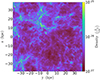 |
Fig. 1. Mass-weighted projection of the gas density in the simulation at z = 18. |
3.1. The halo mass function
The halo mass function (HMF) dn/dM is defined as the number of halos of mass M per unit volume per mass interval. Depending on the primordial power spectrum and the physics of the growth of perturbation assumed, the halo mass function can be computed theoretically. The Sheth-Tormen (ST) formalism (Sheth & Tormen 2002) provides an analytic function that we can compare to the mass function identified in our simulation. In particular, we first want to check that our simulation reproduces the HMF of low-mass halos (105 − 106 M⊙) where primordial star formation is supposed to occur (Yoshida et al. 2003; Park et al. 2021). We highlight the difficulties of reproducing the halo mass function in Appendix A.
First, we show a comparison between the simulated and theoretical HMF at redshift 18 in Fig. 2. At z = 18, the simulation and theory are in good agreement, particularly in the low-mass regime, down to the resolution limit (8.1 × 10⁴ M⊙). There is a minor lack of halos at the high-mass end. Also, as stated in this study, the ST mass function overpredicts the abundance of rare objects at all times by up to 50% compared to the simulations. Overall, the simulation reproduces the halo mass function in the range of interest quite well, namely, between ∼8 × 10⁴ M⊙ and a few 106 M⊙.
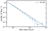 |
Fig. 2. Comparison of the Sheth-Tormen mass function (dashed line) and the one determined in our simulation at z = 18 (solid line with circle). The error bars shows the Poissonian error. The simulation is in good agreement with the analytical halo mass function. |
The second point we want to verify is whether the number of halos detected is statistically representative. Figure 3 shows the number of halos detected above 8 × 10⁴ M⊙ and 7 × 10⁵ M⊙. We chose these two mass thresholds as 8 × 10⁴ M⊙ is our resolution limit and 7 × 10⁵ M⊙ is the critical mass for a halo to host star formation found by Yoshida et al. (2003) and Park et al. (2021). The number of simulated halos converges with the theoretical expectancy with decreasing redshift. This behaviour is expected as halos of constant mass corresponds to smaller peak as redshift evolves in a box of constant size. The gap at high redshift can be explained with cosmic variance.
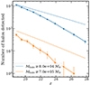 |
Fig. 3. Number of halos detected above 8 × 10⁴ M⊙ and 7 × 10⁵ M⊙ in our simulation box. The dashed lines are the theoretical prediction from the Sheth-Tormen mass function, while the solid lines with circular points are the results from our simulation. The errorbars are the Poissonian error. |
At z = 18, we detect 1376 halos more massive than 8 × 10⁴ M⊙ and around 60 halos with M ≥ 7 × 10⁵ M⊙ in the fiducial simulation. Furthermore, we identified 73 clumps with the clump finder. We never detect more than one clump in a given halo. Over our sample, the mean number of cells forming a clump is 105 (the largest number is 2.6 × 10⁵, the smallest 1.3 × 10⁴). In the following sections, we explore in detail why only 5% of halos host a clump and how it mostly appears to do with the halo mass. The detection of such a high number of halos confirms that size and resolution of our our simulation are well suited for a statistical study. In Appendix A, we present in a resolution study and we show that our fiducial case is convergent when the resolution is improved.
3.2. Clump gravitational stability
We can now verify that by computing the virial parameter αvir whether they are gravitationally unstable or not. This parameter states whether a clump is self-supported (αvir ≳ 1) or is collapsing (αvir ≲ 1). For a spherical cloud with uniform density, it is expressed as:
 (18)
(18)
with cs the sound speed, σvel the velocity dispersion, R the half-mass radius, and Mclump the mass of the clump (sum of the baryonic and DM mass). Sound speed and σvel are of a similar order of magnitude, between 1 and 10 km.s−1 in the typically detected clumps.
Figure 4 shows αvir versus the baryonic mass of each clump at z = 18. All the detected clumps have αvir ≤ 3 and the mean value is ⟨αvir⟩≈0.3. By definition, we observe a strong correlation with the mass of the clump. Indeed, the mass is the main parameter as molecular cooling sets the clump temperature. Overall, nearly all the detected clumps are gravitationally unstable, and therefore are indeed collapsing.
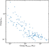 |
Fig. 4. Clumps virial parameter αvir versus the baryonic mass at z = 18. |
However, the detected clumps are not spherical (and also not with a uniform density), but using theses two assumptions are a conservative estimate. For a given cloud, R and, hence, αvir would be smaller if the same mass was packed into a sphere. Also, the gas is denser at the centre of a cloud, which increases the gravitational energy compare to the uniform case. Omitting theses two assumptions would in both cases decrease αvir and would not change the conclusions of presented here.
3.3. Gas accretion and shocks
As gas falls onto the halo, it is heated to its virial temperature with a mild shock. First, Fig. 5 shows maps of one collapsing halo at z = 18 of mass Mvir = 8.7 × 10⁶ M⊙. The gas is accreted though large-scale filaments which can be seen in the leftmost map of gas density. Then, as collapsing molecule formation is triggered and gas starts to be enriched in H2 and HD. Thus, its temperature rapidly decreases to reach a few hundred K.
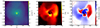 |
Fig. 5. Maps of a halo at z = 18 of mass Mvir = 3 × 10⁶ M⊙ and Tvir = 5.7 × 10³ K. The first map shows the gas density, the middle one the gas temperature and the rightmost one a map of H2 mass fraction. Every property is computed from a mass-average in a slice 30 pc deep. The red circle is the virial radius of the halo. The density map shows the gas collapsing from larger scale, channeling along filaments into the halo. At roughly the virial radius, the gas is heated and starts to pile up. Then, as molecule formation is triggered, gas starts to cool down. Despite the much higher density in the centre of the halo of ∼105 cm−3, the gas is much colder, reaching a few hundred K. Here, in the densest region, the H2 mass fraction reaches ∼10−3. The gas temperature correlates strongly with the H2 fraction, revealing the importance of H2 for cooling. |
Figure 6 shows the phase-space distribution of gas within the virial radius of one halo of mass Mvir = 3 × 10⁶ M⊙ and Tvir = 5.7 × 10³ K. The gas in the halo reaches a density of nH = 105 cm3 and xH2 reaches a plateau at xH2 ≃ 103 cm−3 (second panel from left). The HD mass fraction is much more scattered, around xHD ∼ 10−5. At such densities, molecule formation enables the gas to cool down to 100 K at the most (still hotter than the CMB limit at this redshift of TCMB ≃ 50 K). The drop of xHD at nH ≥ 10−5 is caused by the temperature: HD formation is more efficient at lower temperature and the temperature is still high in this halo at nH = 105 cm−3
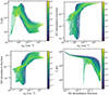 |
Fig. 6. Phase diagrams of the gas within the virial radius of the halo of Fig. 5. We show the temperature, H2 fraction, and HD fraction versus the gas density and the temperature versus the H2 fraction. The logarighmic colormap is weighted with the mass of the gas within each bin. |
The leftmost panel shows that the maximum temperature is ≈104 K, somewhat higher than the virial temperature of this halo. We find that these values are explained by a shock at smaller scales, as Fig. 5 shows. There is a shock at around 10 pc from the halo centre, in the south part of the halo. The temperature reaches more than 104 K. This shock heats up the gas to this temperature as the density increases dramatically (T ∝ ργ − 1). Figure 6 is mass-weighted, so we can see that only a small mass fraction of the gas is shocked at such high temperatures. We observe a similar behaviour in all halos more massive than 1 × 10⁶ M⊙, namely, with gas shock-heated above the virial temperature at the halo centre.
Flower (2001) model the collapse of the initial phases of free-fall collapse in the primordial gas. They find that the infall velocity is strongly supersonic at density nH = 102 cm−3. Here, we observe a slighlty lower density nH ≃ 101 cm−3. They also observe longer H2 cooling rate in the shocked region. Here, the shock is destroying H2, as can be seen on the xH2 versus Tgas panel (on the far right): the gas with the highest temperature (T ≥ 7 × 10³ K) also has the lowest xH2 (xH2 ≤ 10−6).
Kiyuna et al. (2023) also observe a shock in their 3D simulation. However, in their simulation the density of the shock jumps very rapidly from 1 − 10 cm−3 to 104 − 105 cm−3. We did not observe this behaviour in our simulation. However, we stopped our simulation at z = 18 and the most massive halo is 8 × 10⁶ M⊙, which is less than the critical mass for the first emergence of the cold accretion flow found in their simulation, which explains why we cannot observe the shock at high density.
We also study the state of the gas as a function of the distance to the centre of the halo. Figure 7 shows mass-weighted averaged profiles of the gas density, temperature, and inflow velocity of a few halos. The chosen halos are at z = 18 and with masses of [2.7, 3.9, 7.4, 8.8] × 106 M⊙ and virial radius of [2.2, 2.5, 3.1, 3.3] × 102 pc, respectively. To compute the profiles, we mass-average the properties on spherical shells centred on the centre of mass of each halo. As gas is getting closer to the centre of the halo, its density increases (top panel of Fig. 7). First as there is no coolant, the temperature increases adiabatically and reaches a value close to Tvir. The virial temperature of a spherical top-hat collapsing perturbation is fitted in Barkana & Loeb (2001) and is written as:
![Mathematical equation: $$ \begin{aligned}&T_{\mathrm{vir} } = 1.98 \times 10^4 \left(\frac{\mu }{0.6}\right) \left[\frac{\Omega _{\mathrm{m} }}{\Omega _{\mathrm{m} }^{z}}\frac{\Delta _{\mathrm{c} }}{18\pi ^{2}}\right]^{1/3} \nonumber \\&\qquad \times \left(\frac{h \, M_{\mathrm{vir} }}{10^{8}\,{M_{\odot }}}\right)^{2/3} \left(\frac{1+z}{10}\right)\,\mathrm{K} , \end{aligned} $$](/articles/aa/full_html/2024/05/aa47918-23/aa47918-23-eq28.gif) (19)
(19)
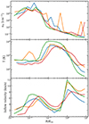 |
Fig. 7. Profiles of mass-weighted average density, gas temperature and radial velocity of a sample of halos at z = 18. The gas temperature is volume-weighted and the inflow velocity is mass-weighted. The horizontal lines are the virial properties of the halo: in the upper panel, the virial temperature; in the lower panel, the virial velocity. |
with  , Δc = 18π2 + 82d − 39d2,
  , μ is the mean molecular weight (equal to 1.2 for monoatomic primordial gas), Mvir is the virial mass of the halo, z is the redshift, and h is the reduced Hubble constant. The gas then forms a bubble of hot gas with a fairly flat temperature profile. Indeed, as shown in the bottom panel, the radial velocity drops sharply. This hot phase of the gas can be seen in Fig. 5 and is deficient in H2 which impeaches the gas from cooling. Then, at a higher density, molecule formation starts to enable the gas to cool down but the size of the dense gas cloud is too small (the half-mass radius is between 5 and 15 pc), seen in Fig. 7.
In the velocity profiles (bottom panel of Fig. 7), we compare against the expression from Barkana & Loeb (2001). They compute the velocity from the virial theorem as:
![Mathematical equation: $$ \begin{aligned} V_{\mathrm{vir} } = 23.4 \left[\frac{\Omega _{\mathrm{m} }}{\Omega _{\mathrm{m} }^{z}}\frac{\Delta _{c}}{18\pi ^{2}}\right]^{1/6} \times \left(\frac{h \, M_{\mathrm{h} }}{10^{8}\,{M_{\odot }}}\right)^{1/3} \left(\frac{1+z}{10}\right)^{1/2}\,\mathrm {km \, s}^{-1} ,\end{aligned} $$](/articles/aa/full_html/2024/05/aa47918-23/aa47918-23-eq31.gif) (20)
(20)
with the same parameters as in Eq. (19). At large scales, the gas is falling toward the halo and its velocity nearly reaches the virial velocity. Then, just inside the virial radius, the radial velocity drops sharply.
3.4. Properties of star-forming primordial halos
We now investigate the properties of the star-forming halos in our simulation with the aim of finding statistically relevant criteria for halos hosting clumps, both in term of physics and chemistry. Previous works highlight a critical threshold in molecular abundance and a mass threshold. We seek to confirm theses results with our simulation.
3.4.1. Chemical properties of halos hosting a cold gas clump
The only chemical species likely to cool the gas are H2 and HD. As the abundance of HD is negligible compared to H2, cus on the molecular hydrogen number fraction xH2, which is expected to determine the onset of cooling. We compute xH2 with a mass weighted-average of the gas within the virial radius. Before the onset of molecular cooling, the temperature of the gas is set by the virial temperature of the halo which can be computed analytically. The virial temperature is computed from Eq. (19).
We plot the mean H2 mass fraction versus the virial temperature in Fig. 8. Red circles correspond to halos hosting cold gas clumps detected by the HOP algorithm and the blue to the ones without a clump. We clearly identify a threshold xH2, crit ≃ 2 × 10⁻⁴ above which a halo is always hosting a clump, in agreement with (Yoshida et al. 2003; Tegmark et al. 1997).
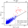 |
Fig. 8. Mass-weighted H2 fraction, xH2, versus virial the temperature for all halos. The red circles are halos hosting clumps and the blue ones are those without them. The black dashed line is a power law fit for the blue points, i.e. halo without clumps. |
Figure 8 shows two different trends. First xH2 increases quite regularly with Tvir, as the halo is accreting mass until ≃2 − 3 × 10³ K, which corresponds, at this redshift, to virial masses of ≃8 × 10⁵ − 106Mvir. We fit with a power law xH2 versus Tvir only for the halos that do not host clumps, namely, the blue points. We find that xH2 scales as T1.47, in fairly good agreement with the scaling of T1.52 found by Yoshida et al. (2003) and Tegmark et al. (1997). The computed slope depends on the chemical network used and can be computed analytically. Tegmark et al. (1997) model H2 formation via the H− channel as a function of the temperature of the gas which is equal to the halo virial temperature before the onset of molecular cooling. The H− channel is the main route of H2 formation in our physical conditions. Its effective formation rate, kH2, depends on the coefficient rate of the reaction forming H2 divided by the one destroying H−. Following Tegmark et al. (1997) in assuming that the molecular fraction is xH2 ≪ 1, it depends only on the gas temperature and is expressed as:
 (21)
(21)
where ki in the rate of reaction i which depends either on the gas temperature or on the radiation temperature for the photoionisation reactions. In the range of temperature between 10 K and 104 K, this rate can really close to be proportional to T1.52, in agreement with the observed rate in our simulation.
Then, when a halo starts to host a clump, the scatter in the plot increases dramatically and the relation with Tvir breaks. Indeed, the assumption that the molecular fraction is negligible is no longer valid. Also, the gas temperature is no more set by the virial temperature as H2 cooling starts to play a role. This trend was not observed in Yoshida et al. (2003) as they find that xH2 continues to increase regularly, independently of the presence or absence of a clump. Recently, Regan (2023) who performed a numerical simulation of the first halos also observe a similar trend as here: the scatter in the cooling time increases above a few times 106 M⊙, similar to our simulation.
Figure 8 only reports one simulation snapshot, at z = 18. We investigate whether the critical xH2 identified is independent of redshift. The lower panel of Fig. 9 shows the evolution over redshift of the minimum H2 mass fraction of halos hosting clumps. The minimal xH2 does not depend on the redshift and is roughly constant at ≃2 − 3 × 10⁻⁴. The dashed lines show the evolution of individual halos, as we trace them forward across snapshots. For these individual halos, the H2 fraction increases and reaches an upper limit of ≃2 − 3 × 10⁻³. This upper limit is probably due to xH2 being computed at the virial scale and to the fact that the simulation does not resolve the densest gas, which is expected to become fully molecular above 1010 cm3.
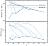 |
Fig. 9. Minimum mass (top) and minimum xH2 fraction (bottom) of halos hosting clumps in our simulation as a function of redshift. The blue solid lines show the evolution of these minimums and the dashed lines show the subsequent mass or xH2 evolution of the relevant ’minimal’ halo, usually increasing in both mass and H2 fraction. In the top panel, the horizontal lines show the critical mass found by Yoshida et al. (2003) and Machacek et al. (2003). |
3.4.2. Physical properties of halos hosting cold gas clump
The minimal mass, Mcrit, of a halo hosting star formation is the main property we investigate here. This critical mass has been inferred from theoretical predictions (Tegmark et al. 1997). It can be used to estimate the global primordial star formation rate. For example, Chantavat et al. (2023) use a redshift-dependant equation to compute the abundances of pop III. In their 3D simulation, Yoshida et al. (2003) investigate the minimal mass and find Mcrit = 7 × 10⁵ M⊙, independent from redshift. Similarly, Machacek et al. (2001) find a critical mass of ≃3 × 10⁵ M⊙ in a 3D simulation.
The upper panel of Fig. 9 shows the minimum mass of halos hosting gas clumps in each output. We infer a minimum mass of ∼1 − 5 × 10⁵ M⊙, which only weakly depends on the redshift. Our higher resolution simulation agrees well with this result from the fiducial simulation, as we show in Appendix A. The value we find is in fairly good agreement with previous simulations, as the value found here is between the results from Yoshida et al. (2003) and Machacek et al. (2001).
The baryonic fraction, fb, is also expected to have an influence. Figure 10 shows a histogram of the baryonic fraction for the all sample of halos (blue) and those with clump (red) with the Poissonian error bars. We observe a clear threshold of fb, crit ∼ 10−1 for a halo to host a clump.
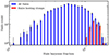 |
Fig. 10. Histogram of the probability density of the baryonic fraction for the all population of halos (blue bars) and those hosting clumps (red bars). Error bars correspond to the Poissonian error. |
3.5. Halo formation history and accretion rate
The presence of a clump is first dictated by the virial mass (or, alternatively, the molecular fraction xH2, which is also correlated to virial mass, see Fig. 8). However, there is a range of masses where there exist halos with and without clumps, therefore, we want to look at other halo properties that can distinguish between these two classes of halos in the mass range where there is an overlap.
We first focus on the halo history and accretion rate. Indeed, the growth of halos via accretion and mergers can be violent and thus have an impact on their properties and star formation. If slow accretion tends to favor equilibrium within the halos, a merger of two DM halos can affect the thermal and chemical evolution of the gas. To study the effects of accretion and mergers, we follow the evolution of individual halos and compare those that form clumps and those that do not.
3.5.1. Halo history
We can study the evolution of halos to see if a higher accretion rate, which heats the gas, delays the presence of a clump. Figure 11 shows the evolution of a random sample of halos hosting clumps at z = 18 (top row) and another subset of halos that do not (bottom row). For both, the right panel shows the evolution of the virial mass as a function of the redshift and the left one gives the H2 abundance as a function of the volume average gas temperature. In the top row, the boundary between the solid and the dashed circles marks the first snapshot at which a halo hosts a clump. The first row reflects Fig. 9 as we can clearly see a threshold in both the virial mass and xH2 above which a halo hosts a clump. The threshold is much clearer for xH2 as there is a wider range in Mvir for which there exists halos both with and without gas clumps. None of the halos without cold gas clumps reaches either of these thresholds (M ≥ 7 × 10⁵ M⊙ or xH2 ≥ 2 × 10⁻⁴).
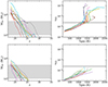 |
Fig. 11. Evolution of halos across snapshots. Top: sample of halos hosting clump at z = 18.8, left: halo virial mass vs redshift, right: halo H2 abundance vs mass average gas temperature. The boundary between the solid line and dashed line corresponds to the snapshot at which a halo first host a cold gas clump. Bottom: same plot for a sample of halos that do not host cold gas clump. The gray rectangle shows the interval in the crirical value of Mvir and xH2 identified in Sect. 3.4. |
The plot of xH2 versus the gas temperature highlights three phases in the halo evolution. First, as the halo accretes mass and is collapsing, its temperature increases adiabatically as it cannot exchange heat with the surrounding medium. Then, once it reaches the critical temperature for H2 formation (∼1 − 1.5 × 10³ K), H2 starts to play a role and to cool down the gas. However, at the same time, the halo is still accreting gas which acts as a heating term, counterbalancing the effect of H2 cooling. This explains the vertical part of the trajectory. Finally, H2 formation starts to saturate and the halo heats up again as cooling cannot compensate dynamical heating. Overall, the halo history seems to have only a limited impact.
3.5.2. Accretion rate
We can also directly study the impact of the accretion rate in a given snapshot. For this, we show in Fig. 12 the accretion rate at the virial radius versus the virial mass of halos. We computed the accretion rate with the difference of mass of each halo between two snapshots. Again, the red points correspond to halos that host cold and dense clumps and the blue ones those that do not. The accretion rate is computed between two snapshots at z = 18 and z = 18.8. First, we can clearly see that at a given mass, halos that host cold gas clumps tend to have a smaller accretion rate. This is especially true at the critical mass close to ≃106 M⊙ where a halo first hosts a clump.
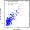 |
Fig. 12. Virial mass versus the accretion rate at the virial radius at z = 18. The red circles are halos hosting clumps and the blue ones those without. The green dotted line shows |

Following Yoshida et al. (2003), we computed a critical accretion rate by comparing the heating due to the accretion to the H2 cooling. The dynamical heating due to the accretion rate can be linked to the increase of the virial temperature of the halo as follows:
 (22)
(22)
where we use Eq. (19) for the second equality, α depends on the factors of this equation. The temperature of the gas could be different from the virial temperature, but the two are equal before the onset of H2 cooling. The H2 cooling rate is:
 (23)
(23)
where ΛH2 is the molecular hydrogen cooling rate.
If the cooling and heating terms are equal, a halo cannot cool down and, thus, clump formation is delayed. The molecular cooling rate only depends on the abundance of H2, which can be assumed constant in our restricted mass range and ΛH2, which is roughly proportional to T2 between 100 and 5000 K as we use the cooling rate from Glover & Abel (2008). Equalling the two rates gives a critical accretion rate above which a cloud cannot cool down thanks to molecule cooling. As  , the crirical growth rate reads as
  . Figure 12 shows that this relation is valid above 5 × 10⁵ M⊙ but breaks for less massive halos. Indeed, in this case, the limiting factor is the mass of the halo.
3.6. Spin parameter
We computed the angular momentum  with the classic expression:
 (24)
(24)
with  as the position of the DM particle or centre of gas cell, i, with respect to the clump barycentre (which is not necessary the same as the halo barycentre), mi is the mass of the particle or cell, and
  its velocity relative to that of the clump. We compute
  both for the DM and the baryons.
The angular momentum depends sensitively on the mass of an object, as Eq. (24) is a sum. Moreover, more massive objects have higher rotational velocities. Therefore, to compare the rotational support of halos with a wide range of mass, we would need a more appropriately weighted physical quantit : we chose to compute the spin parameter, following the definition from Bullock et al. (2001),
 (25)
(25)
with  , where G is the gravitational constant, M is the mass of the object, and R is the radius in case of a circular object. Also, J⋆ and M⋆ are the angular momentum in the halo frame and the mass of the considered particles (either the gas or the DM in our case), J⋆/M⋆ is the specific angular momentum. For the DM, we computed the spin parameter using the virial properties Rvir and Mvir. For the baryons, we computed the angular momentum and the mass over all cells within a sphere centred of the centre of mass and of radius, Rvir. Numerical studies (Bromm et al. 2002; Hirano et al. 2014) have highlighted the importance of the angular momentum and, thus, of the spin parameter, as both of these aspects may influence the collapse of the gas cloud.
Figure 13 shows the correlation between the spin parameter from the DM and that of the baryons in our simulation at z = 18. The red points are the halos hosting gas clump and the blue one show the ones without. As shown by the two histograms, the distribution of the spin parameter follows a lognormal distribution:
 (26)
(26)
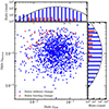 |
Fig. 13. Spin parameter for the DM versus the baryonic one at z = 18. The red points are the halos hosting clump. On top and on the side are the distribution for the two quantities, again red are halos with clump and blue the all distribution of halos. The histograms are fitted with a lognormal distribution (black curve), with the parameters |


We find  and
and  . The fitted value for the DM is in agreement with Sasaki et al. (2014) and Yoshida et al. (2003). Furthermore, Sasaki et al. (2014) performed high-resolution DM-only simulations with the code GADGET-3 to study the properties of DM halos. The spin parameter is of the same order of magnitude for the two components and we observe a larger scatter in the spin of the baryons than for the DM. There is no correlation between the two components. de Souza et al. (2013) also found a much weaker correlation at this redshift compare to lower redshift as the two components have more time to interact and redistribute angular momentum at lower redshift. From the probability distribution function (PDF) of the two components, we see that halos hosting clumps tend to have a lower DM spin parameter and a higher baryonic one.
The angle between the angular momentum of the DM and the baryons, θ, can reveal the degree of interaction between the two components. Figure 14 shows the distribution of θ for all halos and those hosting clumps for the three last snapshots (at z = 19.5, 18.8 and 18)1. The distribution shows a trend with a peak at 40° and a slow decrease toward larger angle. The average value is roughly 70° for all halos and for halos hosting clumps, meaning that the DM and baryons velocity fields are not aligned. The distribution of the angle is the same for the two populations of halos.
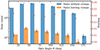 |
Fig. 14. Histogram of the probability density of the angle θ between the DM and baryonic angular momentum vectors for halos without clumps (blue bars) and halos hosting clumps (red bars) for the three last snapshots (corresponding to redshifts 19.5, 18.8 and 18). Error bars correspond to the Poissonian error. The fraction on the right-axis corresponds to the ratio of the number of halos hosting a clump versus the total number of halos. |
3.7. Shape and triaxiality parameter
We are also interested in the shape of the detected halos and clumps. To do so, we compute the triaxiality from the gas and the DM component. Indeed, the free-fall time of a collapsing object depends on its aspect ratio (Pon et al. 2012), thus on its triaxiality. The triaxiality also gives a rough estimate of the shape, mainly the oblateness and prolateness of a clump.
3.7.1. Halo virial scale
To compute the triaxiality, we need to find the eigenvalues of the inertia tensor I. We compute the inertia tensor with the classic definition, as used by de Souza et al. (2013),
 (27)
(27)
where ri and mi are the distant with respect to the halo centre and the mass of a DM matter or a gas cell, while δjk is the Kronecker delta. The sum is computed over all cells and particles of a given halos, N is the number of elements.
The eigenvalue value from I, a ≥ b ≥ c correspond to the axis ratio of an ellipsoid representing the equivalent homogenous shape of the halo. The axis ratio can be normalize, to account for the sphericity, s = c/a (a spherical halo has s = 1), the oblateness, q = b/a, and the prolateness, p = c/b. From this definition, the triaxiality is:
 (28)
(28)
if q = 1 (meaning a = b ≥ c), T → 0 and the halo is shaped like an oblate (disk-shaped), whereas if p = 1 (meaning a ≥ c = b), T → 1 and the halo is shaped like a prolate (filament-shaped).
We computed the triaxiality parameter for the DM component of every halo. Figure 15 shows a plot of the halo DM spin parameter versus the triaxiality parameter with an histogram for both quantity. The distribution of the triaxiality parameter shows that most halos are prolate, namely, they have a filamentary shape. This is coherent with theories predicting halos to accrete matter from filaments. There is a trend linking a higher triaxiality parameter to a higher spin parameter.
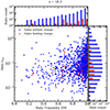 |
Fig. 15. Spin parameter versus the triaxiality parameter in our simulation, at z = 18 for the halos. |
3.7.2. Cold and dense gas scale
We go on to investigate the properties of the gas at much smaller scales. Our simulation is able to resolve the gas, until nH ∼ 105 cm−3, where the gas is unstable and collapsing. It is interesting to study the local properties of the dense gas, as these will be the initial conditions for future zoom-in and isolated high-resolution simulations.
We computed the spin and the triaxiality parameter for the dense gas clouds following the previous formulation. Here, we computed it only for the gas denser than 100 cm−3 to focus on the densest phase within a clump. This threshold corresponds to the point where molecular cooling is the most efficient; thus, the lowest temperature is achieved, which can be seen on the phase diagram. The distribution of the triaxiality parameter is shown in Fig. 16. It is different from that of the halo distribution (see Fig. 15). Here, the distribution is much more uniform.
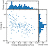 |
Fig. 16. Spin parameter versus the triaxiality parameter for the gas clouds, at z = 18. |
The distribution of the triaxiality parameter is nearly uniform between 0 and 1, contrary to the distribution at the halo scale. The presence of oblate geometry of the gas at higher density indicates that some clumps are rotationally supported. Gao et al. (2007) also found such a trend in their simulation. They performed high-resolution cosmological simulations to study the birth site of primordial stars. We observe a slight trend between a larger spin parameter and a larger triaxiality. A higher triaxiality parameter means a more pronounced disk shape, which is expected to be more rotationally supported and thus have a larger spin parameter. We find no correlation between the spin of the dense gas and the one computed at the virial scale from the baryons. The large-scale spin does not seem to be connected with the dynamic of the gas once it has cooled.
3.8. Cooling species
Our chemical network includes two cooling species, HD and H2. As H2 is much more abundant than HD, the cooling is mainly driven by H2 in most cases. However, previous studies (Ripamonti 2007; Greif et al. 2011) have identified cases where HD cooling is effective; HD can further cool the gas, even to the CMB floor. This HD-cooling mode has also been identified by Hirano et al. (2015) in their 3D hydrodynamic simulations. Following this study and that of McGreer & Bryan (2008), we can split the halos into HD-cooling ones and others. We chose to differentiate between these two types of halos by fHD/fH2 ≥ 10−3, where fHD (resp. fH2) is the HD (resp. H2) mass-fraction of the halo computed for the gas inside its virial radius. We only considered halos with a clump for this analysis as they are the ones directly related to this kind of HD cooling. Of the 73 halos hosting clumps detected at z = 18, 36 are HD-cooling, meaning nearly half of them host a high HD fraction. We observe that this ratio tends to increase with redshift, starting from roughly 30% at z = 22 to 50% at z = 18. We observed a slightly higher fraction compared with the 10% fraction found in Hirano et al. (2015). We think this might be due to the selection criteria, as we restricted our sample to halos where we detected a clump. Indeed, we have a fraction of 10–12% of HD-cooling halos when we consider all halos more massive than 4 × 10⁵ M⊙.
A higher HD fraction is linked with a lower gas temperature among our halo sample. Figure 17 shows the average profile from various halos with different fHD/fH2. All halos showed on this plot have similar mass, between 1.4 × 10⁶ M⊙ and 1.6 × 10⁶ M⊙. However, their ratio fHD/fH2 differs at the virial scale, as indicated by the color bar on the right. Then, fHD/fH2 is between 4 × 10⁻⁴ and 2.2 × 10⁻³, meaning that some halos are HD-cooling ones. The bottom plot from Fig. 17 clearly shows that in the HD-cooling halos, HD formation is only triggered at high density, nH ≥ 102 cm−3, ie at low temperature Tgas ∼ 1 − 5 × 10² K (upper panel), which is what we expect from theory. The upper panel in Fig. 17 clearly shows that HD-cooling halos are colder, nearly reaching 102 K at nH = 104 cm−3, which is still above the CMB cooling limit at this redshift (∼50 K). We see that HD cooling is non-negligible in the range of 102 − 106 cm−3 in our simulation, which is in agreement with McGreer & Bryan (2008). Overall, these results are consistent with those from Hirano et al. (2015), Greif et al. (2011).
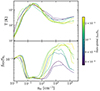 |
Fig. 17. Average profile of primordial halos at z = 18. The top plot shows the mass-average gas temperature versus the density, the bottom gives fHD/fH2 versus the gas density. The color map corresponds to fHD/fH2. All halos have similar mass, between 1.4 × 10⁶ M⊙ and 1.6 × 10⁶ M⊙. The only difference among theses is fHD/fH2, which is indicated via the line color and the color bar on the right. fHD/fH2 is computed via a mass-average mean of the gas within the virial radius. |
Small differences at the halo scale can be amplified in the collapse and lead to different properties of the star-forming region, in particular the HD fraction. In our simulation, it is not clear what is causing a higher HD fraction in some halos. At the clump scale, we find that a higher fHD/fH2 is correlated with a lower spin parameter. Figure 18 shows a plot of the mass-average fHD/fH2 versus the spin parameter for each clump of the simulation at z = 18. We observe a trend linking a higher spin parameter and a higher HD fraction within a clump. One explanation for this behaviour is that the collapse is slower for a rapid rotating cloud which could lead to an enhanced HD formation and more cooling. With a prolonged collapse, there is an extended window for molecular cooling since the creation of molecules does not happen instantly. Furthermore, HD formation is enhanced at low temperature, hence, there is a higher fHD/fH2 ratio for slow collapse. This mechanism has been observed by Nishijima et al. (2023) and could be efficient here.
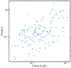 |
Fig. 18. Mass-average fHD/fH2 versus the specific spin parameter for each clump of the simulation at z = 18. The color coding is the same as before and depends on the threshold. |
3.9. Spatial distribution of halos hosting clumps
We have seen that halos hosting star formation have particular physical and chemical properties, in particular, there is a clear mass threshold for a halo to host a cold gas clump. The search for population III birth sites is a search for the most massive halos. However, the properties of halos can be influenced by their environment. For example, Gao et al. (2005) found that halos assembled earlier are much more clustered and Sasaki et al. (2014) found that clustered halos have a higher spin parameters due to stronger tidal forces. To study this point, we computed the two-point correlation function as it highlights such clustering effects. We compared the correlation function for halos with clumps to that of all halos with masses above our resolution limit. We followed the method from Hamilton (1993), who computed the correlation function ξ(r) from two catalogues, with the first following a random uniform distribution and that of the simulation. With this, ξ(r) is expressed as:
 (29)
(29)
where DD(r), RR(r), and DR(r) are the number of pairs separated by a distance, r, respectively in our simulation (halo-halo pairs), in the random distribution (random-random pairs) and between the random and simulated catalogue (random-halo pairs).
Figure 19 shows the two-point correlation function of three categories of halos: all halos (blue dotted line), halos hosting clumps (orange solid line), and halos more massive than Mcrit = 1 × 10⁶ M⊙. Halos hosting clumps are as much clustered as the ones more massive than 1 × 10⁶ M⊙. The mean separation between two halos hosting clumps is only 0.5 pkpc. The correlation function of halos hosting star formation is coherent with that of halos more massive than 1 × 10⁶ M⊙, the threshold identified previously. The presence of a clump is not influenced by the clustering of a halo. Then, as massive halos are more clustered than all halos, we observe the same behaviour for halos with clump.
 |
Fig. 19. Two-point correlation function of halos in our two simulation at z = 18. The dashed blue line shows that of all halos detected, the orange solid line with circles gives that of halos hosting clumps, and the green dashed line with crosses gives that of halos with Mvir ≥ 1 × 10⁶ M⊙. |
4. Discussion
4.1. Birth sites of primordial stars
Our cosmological simulation enables us to probe the condition in which primordial stars were born. The minimum mass for halos hosting star formation we derive in our simulation is consistent with previous results. The minimum mass is primarily set by the fraction of molecular hydrogen produced in the DM halos, which is linked to its virial temperature. Because of the limited volume of our simulation (1 h−1cMpc), we are not able to capture the very first star-forming halos, appearing in rare density fluctuations (σ ≥ 4) of the Gaussian density field. They were probably born at much higher redshift (z ≥ 30) than this study can capture. However, they are extremely rare and so, they are not representative of the global primordial halo population. In order to resolve the birth of the first primordial stars, we would need either a much larger box size or to artificially simulate an over-dense region of the Universe.
The chemical properties of halos hosting collapsing gas clumps are quite universal concerning molecular hydrogen. In all of those halos, we observe a similar H2 fraction. However, we observe differences in the HD fraction, which are linked with a higher degree of rotation at the star-forming cloud scale.
4.2. Caveats
In our simulations, we did not include streaming velocities between baryons and DM. The relative velocity decreases with the redshift as vstream ∝ (1 + z). Druschke et al. (2020) found that streaming velocity has a negligible effect on the spin and shape of the DM component in mini-halos, but strongly affects the gas component. Its spin parameter increases and it is less spherical. Simulations studying the link with primordial star formation shows that it delays the formation of the first pop III stars. Schauer et al. (2019) study this effect in a cosmological simulation. There results without streaming velocity are in agreement with our work, but when they include non-zero streaming velocity the minimum mass for halo formation is increased by a factor of a few. In the most extreme case, star formation occurs exclusively in atomic cooling halo, with Tvir ≥ 104 K. This point is left for future studies.
We also do not include magnetic fields in our cosmological simulation. The mean magnetic field of the early Universe is not constrained. Even the presence of any magnetic field before the first stars is in question (Attia et al. 2021). Stacy et al. (2022) compute the primordial IMF with magnetic field. They start from a uniform field B0 = 4.5 × 10⁻¹² G at z = 54. The growth of the field is then nearly proportional to n2/3 in the range 10−2 − 108 cm−3, reaching 10−2 G at nH = 108 cm−3. The effects of magnetic field are negligible is the range of our present simulation. However, Stacy et al. (2022) found that is has a significant influence of the primordial IMF by suppressing fragmentation and, thus, low-mass stars as well. The primordial magnetic field at the halo scale probably requires additional study and further constraints to get coherent seeds at the halo scale.
The first feedback of pop III stars is radiative feedback from the photons emitted by the star. These photons, in particular those in the Lyman-Werner (LW) bands, can photo-ionize and photodissociate molecular hydrogen in a nearby halo. The change in the chemical composition can influence the result of the collapse, to form the so called population III.2 stars (Greif et al. 2008; Hirano et al. 2014): a distinct population of metal-free stars formed in halos illuminated by a neighbouring already formed pop III star. Such background radiation can increase the ionisation fraction and photo-dissociate H2. A higher ionisation fraction acts as a catatalyst for H2 formation but Lyman-Werner photons can also dissociate H2. To study this first feedback, we need to estimate the spatial distribution of halos forming stars. We have seen, in a qualitative sense, that halos hosting star formation are as clustered as other halos, highlighting the role of radiative feedback. The timescale for mechanical and chemical feedback is much longer than the radiative one, but plays a major role in the transition between population III and II stars.
5. Conclusion
In this study, we run a cosmological simulation following the evolution of DM and baryons to study the birth sites of primordial stars. Our study makes it possible to obtain the statistical properties of the low-mass halos hosting primordial star formation. The resolution of our cosmological simulation enables us to resolve the star forming region until sufficiently high density ∼105 cm−3 to ensure the gravitational instability of the cold and dense gas cloud. We use an updated chemical network following the abundances of keys species (e−, H, H+, H−, D, D+, He, H2,  , HD, and HeH+). We now plan to run zoom-in simulations and isolated collapse to sample the IMF with sink particles.
Our analysis is focused on many important properties of the halos, in particular, the distribution of mass, spin, shape, and the chemical properties. We also briefly study the properties of the dense clouds. Our main results can be summarised as follows:
– The gas radial profiles are coherent with the global physical understanding of the accretion mechanism. We observe the formation of a shock at small scales close to the centre of the halo, which heats up the gas to 104 K at nH = 101 cm−3.
– The minimal halo mass for halo hosting pop III star formation is found to be ∼7 × 10⁵ M⊙, in coherence with previous results. We observe a resolution convergence for this lower limit. We also observe a minimum H2 abundance for a halo of xH2 ≃ 2 × 10⁻⁴ at the halo scale.
– Halo history does not have a major impact on clump formation. However, a high accretion rate can slightly delay the presence of star-forming clump.
– The spin parameter of the DM is independent of that of baryons at the halo scale. We also observed no correlation between the direction of the angular momentum for the two components.
– At the halo scale, halos tend to have filamentary shapes. At the clump scale, the distribution of the gas triaxiality parameter is flat. It means that the disk shape is more frequent, which can be due to a larger degree of rotation.
– The HD abundance is not uniform among the halo population. Halos with a higher HD abundance are colder as the temperature in the range 102 − 104 cm−3 depends a lot on the HD abundance. The higher fraction of HD is linked with a higher spin parameter of the dense gas.
We stack three snapshots here to reduce noise due to few halos hosting clumps.
Acknowledgments
We thank Maxime Gontel, Pierre Hily-Blant and Alexandre Faure for their help and for letting us use their chemical network. We gratefully acknowledge support from the PSMN (Pôle Scientifique de Modélisation Numérique) of the ENS de Lyon for the computing resources. The authors are grateful to the LABEX Lyon Institute of Origins (ANR-10-LABX-0066) Lyon for its financial support within the Plan France 2030 of the French government operated by the National Research Agency (ANR). The authors are grateful to the LABEX Lyon Institute of Origins (ANR-10-LABX-0066) Lyon for its financial support within the program “Investissements d’Avenir” of the French government operated by the National Research Agency (ANR).
References
- Attia, O., Teyssier, R., Katz, H., et al. 2021, MNRAS, 504, 2346 [NASA ADS] [CrossRef] [Google Scholar]
- Aubert, D., Pichon, C., & Colombi, S. 2004, MNRAS, 352, 376 [Google Scholar]
- Barkana, R., & Loeb, A. 2001, Phys. Rep., 349, 125 [NASA ADS] [CrossRef] [Google Scholar]
- Bromm, V., Coppi, P. S., & Larson, R. B. 2002, ApJ, 564, 23 [Google Scholar]
- Bullock, J. S., Dekel, A., Kolatt, T. S., et al. 2001, ApJ, 555, 240 [NASA ADS] [CrossRef] [Google Scholar]
- Byrne, G. D., & Hindmarsh, A. C. 1987, J. Comput. Phys., 70, 1 [NASA ADS] [CrossRef] [Google Scholar]
- Cen, R. 1992, ApJS, 78, 341 [NASA ADS] [CrossRef] [Google Scholar]
- Chantavat, T., Chongchitnan, S., & Silk, J. 2023, MNRAS, 522, 3256 [NASA ADS] [CrossRef] [Google Scholar]
- de Souza, R. S., Ciardi, B., Maio, U., & Ferrara, A. 2013, MNRAS, 428, 2109 [NASA ADS] [CrossRef] [Google Scholar]
- Druschke, M., Schauer, A. T. P., Glover, S. C. O., & Klessen, R. S. 2018, MNRAS, 481, 3266 [CrossRef] [Google Scholar]
- Druschke, M., Schauer, A. T. P., Glover, S. C. O., & Klessen, R. S. 2020, MNRAS, 498, 4839 [NASA ADS] [CrossRef] [Google Scholar]
- Eisenstein, D. J., & Hut, P. 1998, ApJ, 498, 137 [NASA ADS] [CrossRef] [Google Scholar]
- Flower, D. R., & Pineau des Forêts, G., 2001, MNRAS, 323, 672 [NASA ADS] [CrossRef] [Google Scholar]
- Forrey, R. C. 2013, ApJ, 773, L25 [NASA ADS] [CrossRef] [Google Scholar]
- Galli, D., & Palla, F. 1998, A&A, 335, 403 [NASA ADS] [Google Scholar]
- Galli, D., & Palla, F. 2013, ARA&A, 51, 163 [NASA ADS] [CrossRef] [Google Scholar]
- Gao, L., Springel, V., & White, S. D. M. 2005, MNRAS, 363, L66 [NASA ADS] [CrossRef] [Google Scholar]
- Gao, L., Yoshida, N., Abel, T., et al. 2007, MNRAS, 378, 449 [NASA ADS] [CrossRef] [Google Scholar]
- Glover, S. C. O., & Abel, T. 2008, MNRAS, 388, 1627 [NASA ADS] [CrossRef] [Google Scholar]
- Grassi, T., Bovino, S., Schleicher, D. R. G., et al. 2014, MNRAS, 439, 2386 [Google Scholar]
- Greif, T. H., Johnson, J. L., Klessen, R. S., & Bromm, V. 2008, MNRAS, 387, 1021 [NASA ADS] [CrossRef] [Google Scholar]
- Greif, T. H., Springel, V., White, S. D. M., et al. 2011, ApJ, 737, 75 [NASA ADS] [CrossRef] [Google Scholar]
- Guillet, T., & Teyssier, R. 2011, J. Comput. Phys., 230, 4756 [Google Scholar]
- Hahn, O., & Abel, T. 2011, MNRAS, 415, 2101 [Google Scholar]
- Hamilton, A. J. S. 1993, ApJ, 417, 19 [Google Scholar]
- Hirano, S., Hosokawa, T., Yoshida, N., et al. 2014, ApJ, 781, 60 [NASA ADS] [CrossRef] [Google Scholar]
- Hirano, S., Hosokawa, T., Yoshida, N., Omukai, K., & Yorke, H. W. 2015, MNRAS, 448, 568 [NASA ADS] [CrossRef] [Google Scholar]
- Kazantzidis, S., Kravtsov, A. V., Zentner, A. R., et al. 2004, ApJ, 611, L73 [Google Scholar]
- Kiyuna, M., Hosokawa, T., & Chon, S. 2023, MNRAS, 523, 1496 [NASA ADS] [CrossRef] [Google Scholar]
- Klessen, R. S., & Glover, S. C. O. 2023, ARA&A, 61, 65 [NASA ADS] [CrossRef] [Google Scholar]
- Lipovka, A., Núñez-López, R., & Avila-Reese, V. 2005, MNRAS, 361, 850 [NASA ADS] [CrossRef] [Google Scholar]
- Lukić, Z., Heitmann, K., Habib, S., Bashinsky, S., & Ricker, P. M. 2007, ApJ, 671, 1160 [CrossRef] [Google Scholar]
- Machacek, M. E., Bryan, G. L., & Abel, T. 2001, ApJ, 548, 509 [NASA ADS] [CrossRef] [Google Scholar]
- Machacek, M. E., Bryan, G. L., & Abel, T. 2003, MNRAS, 338, 273 [NASA ADS] [CrossRef] [Google Scholar]
- McGreer, I. D., & Bryan, G. L. 2008, ApJ, 685, 8 [CrossRef] [Google Scholar]
- McKee, C. F., & Tan, J. C. 2008, ApJ, 681, 771 [NASA ADS] [CrossRef] [Google Scholar]
- Nishijima, S., Hirano, S., & Umeda, H. 2023, ApJ, submitted [arXiv:2311.10386] [Google Scholar]
- Novosyadlyj, B., Sergijenko, O., & Shulga, V. M. 2017, Kinematics Phys. Celestial Bodies, 33, 255 [NASA ADS] [CrossRef] [Google Scholar]
- Omukai, K. 2000, ApJ, 534, 809 [NASA ADS] [CrossRef] [Google Scholar]
- Park, J., Ricotti, M., & Sugimura, K. 2021, MNRAS, 508, 6193 [NASA ADS] [CrossRef] [Google Scholar]
- Planck Collaboration VI. 2020, A&A, 641, A6 [NASA ADS] [CrossRef] [EDP Sciences] [Google Scholar]
- Pon, A., Toalá, J. A., Johnstone, D., et al. 2012, ApJ, 756, 145 [NASA ADS] [CrossRef] [Google Scholar]
- Reed, D. S., Bower, R., Frenk, C. S., Jenkins, A., & Theuns, T. 2007, MNRAS, 374, 2 [NASA ADS] [CrossRef] [Google Scholar]
- Rees, M. J., & Ostriker, J. P. 1977, MNRAS, 179, 541 [NASA ADS] [CrossRef] [Google Scholar]
- Regan, J. 2023, Open J. Astrophys., 6, 12 [NASA ADS] [CrossRef] [Google Scholar]
- Ripamonti, E. 2007, MNRAS, 376, 709 [NASA ADS] [CrossRef] [Google Scholar]
- Sasaki, M., Clark, P. C., Springel, V., Klessen, R. S., & Glover, S. C. O. 2014, MNRAS, 442, 1942 [CrossRef] [Google Scholar]
- Schauer, A. T. P., Glover, S. C. O., Klessen, R. S., & Ceverino, D. 2019, MNRAS, 484, 3510 [NASA ADS] [CrossRef] [Google Scholar]
- Seager, S., Sasselov, D. D., & Scott, D. 2000, ApJS, 128, 407 [NASA ADS] [CrossRef] [Google Scholar]
- Sheth, R. K., & Tormen, G. 2002, MNRAS, 329, 61 [Google Scholar]
- Stacy, A., Bromm, V., & Lee, A. T. 2016, MNRAS, 462, 1307 [NASA ADS] [CrossRef] [Google Scholar]
- Stacy, A., McKee, C. F., Lee, A. T., Klein, R. I., & Li, P. S. 2022, MNRAS, 511, 5042 [NASA ADS] [CrossRef] [Google Scholar]
- Tegmark, M., Silk, J., Rees, M., et al. 1997, ApJ, 474, 1 [NASA ADS] [CrossRef] [Google Scholar]
- Teyssier, R. 2002, A&A, 385, 337 [CrossRef] [EDP Sciences] [Google Scholar]
- Toro, E. F., Spruce, M., & Speares, W. 1994, Shock Waves, 4, 25 [Google Scholar]
- Tweed, D., Devriendt, J., Blaizot, J., Colombi, S., & Slyz, A. 2009, A&A, 506, 647 [NASA ADS] [CrossRef] [EDP Sciences] [Google Scholar]
- Yoshida, N., Sokasian, A., Hernquist, L., & Springel, V. 2003, ApJ, 598, 73 [NASA ADS] [CrossRef] [Google Scholar]
- Yoshida, N., Omukai, K., Hernquist, L., & Abel, T. 2006, ApJ, 652, 6 [NASA ADS] [CrossRef] [Google Scholar]
Appendix A: Halo mass function and the higher resolution simulation
Reproducing the halo mass function from numerical simulations is a real challenge and suffers from a great deal of caveats, especially at high redshift. One difficulty is reaching a high mass resolution in a volume large enough to sample the cosmological mass perturbation spectrum completely. At high redshifts, the effects of the finite box size become particularly important because any overdensities represent rare fluctuations in the spectrum of linear fluctuations (Reed et al. 2007). Also, the box size cuts all larger fluctuations than those that can fit within it. The modes with a large wavelength are thus not present. Another effect linked with the finite box size is the cosmic variance, namely, the run-to-run variations introduced by the finite sampling of density modes. As stated in Lukić et al. (2007), the variance within a same set of simulations can induce variation as much as an order of magnitude. Finally, The parameters of the halo finder can also induce variations. We check (in Section 3.1) how our fiducial simulation reproduces the halo mass function.
Furthermore, we tested the resolution convergence of this simulation with a higher resolution simulation with the parameter stated in Table 1. We plot the halo mass function of the two simulations on Figure A.1 (same format as Figure 2). The sample of the halo mass function is valid until 104 M⊙ in the high-resolution simulation, which further extends our resolution limit.
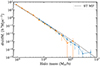 |
Fig. A.1. Comparison of the Sheth-Tormen mass function (dashed line) and the one detected in our two simulations at z = 18 (solid line with circle). The error bars are the Poissonian error bars. |
To test the convergence, we reproduce Figure 9 which shows the minimal mass and H2 fraction of halos hosting cold gas clump. The plot corresponding to the two simulation are shown on Figure A.2. In these two panels, the blue curve is the same as that of Figure A.2. The curve from the high-resolution simulation (the orange line) is in agreement with the blue one, showing that the two simulations agree for the low-mass halo limit.
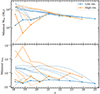 |
Fig. A.2. Minimum H2 mass fraction of halos hosting gas clumps detected with our algorithm. The blue (resp. the orange) line corresponds to the high (resp. the low) resolution simulation. The dashed lines show the subsequent mass or xH2 evolution of the relevant ’minimal’ halo, usually increasing in both mass and H2 fraction with the same color-coding. |
Appendix B: Chemical initial conditions
We computed the chemical abundances at z = 100, thanks to a one-zone model that takes into account the physical evolution of the Universe from z = 104. Our network includes photo-ionisation and photo-dissociation by the CMB photons and it is still valid at higher redshift. Computing the initial chemical abundances in this way enables us to be consistent with our RAMSES-KROME simulation, starting at redshift z = 100.
Chemical abundances at the redshifts, z = 104, z = 103, and z = 100
After the primordial nucleosynthesis, the Universe only consists of hydrogen, deuterium, helium and a tiny fraction of lithium. At a redshift of z = 104, all atoms are fully ionised as the thermal radiation is above there excitations levels (Seager et al. 2000). The recombination starts at a redshift of 1100 and at z = 100, the Universe is nearly neutral. However, the electron fraction and the number density of the molecules is not zero, even at this redshift. To study the formation of the first luminous objects, we need to know the initial chemical abundances of every species. This is of primordial importance as molecular formation is catalysed and strongly enhanced by the ionisation fraction, for example.
We considered a one-zone spherical Universe. The density is assumed to be uniform at all times and it corresponds to the co-moving density : ρ = ΩBρca3, where ΩB is the density parameter, ρc is the critical density, and a is the expansion factor. We set the radiation temperature as: Trad = TCMB × a, with TCMB = 2.73 K (the temperature of the CMB). We started at z = 104, assuming that all species are fully ionised, taking  and
and  . We chose to start the one-zone simulation at z = 104 with all species fully ionised. We took the maximum ionised level for all species: H+, D+, He. Our network does not include He++ and He+, so we started our simulation with only He, which is not realistic at high redshifts, but this choice does not influence the values found at z = 100.
Figure B.1 shows the evolution of abundances of different species of the early Universe. Our results are consistent with simulation of molecule formation in the early Universe (Novosyadlyj et al. 2017) and from other primordial networks.
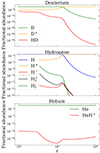 |
Fig. B.1. Evolution of the species as a function of redshift. Top : Deuterium species (D, D+ and HD), Middle : Hydrogen species (H, H+, H−, |

Appendix C: Chemical network
Here, we present the chemical network used in the simulation. Full details about the network, in particular, the rates, will be described in a future paper: Faure et al (in prep.). The molecular abundances, especially those of H2 and HD, were found to be in good agreement with previous studies, suggesting that the dominant (thermal) reaction rate coefficients have reached such a level of accuracy that they are no longer a limiting factor. An important reaction that needs further investigations is the charge exchange between  and H. The full chemical network is available upon request.
Reaction of the chemical network.
All Tables
All Figures
|
Fig. 1. Mass-weighted projection of the gas density in the simulation at z = 18. |
| In the text | |
|
Fig. 2. Comparison of the Sheth-Tormen mass function (dashed line) and the one determined in our simulation at z = 18 (solid line with circle). The error bars shows the Poissonian error. The simulation is in good agreement with the analytical halo mass function. |
| In the text | |
|
Fig. 3. Number of halos detected above 8 × 10⁴ M⊙ and 7 × 10⁵ M⊙ in our simulation box. The dashed lines are the theoretical prediction from the Sheth-Tormen mass function, while the solid lines with circular points are the results from our simulation. The errorbars are the Poissonian error. |
| In the text | |
|
Fig. 4. Clumps virial parameter αvir versus the baryonic mass at z = 18. |
| In the text | |
|
Fig. 5. Maps of a halo at z = 18 of mass Mvir = 3 × 10⁶ M⊙ and Tvir = 5.7 × 10³ K. The first map shows the gas density, the middle one the gas temperature and the rightmost one a map of H2 mass fraction. Every property is computed from a mass-average in a slice 30 pc deep. The red circle is the virial radius of the halo. The density map shows the gas collapsing from larger scale, channeling along filaments into the halo. At roughly the virial radius, the gas is heated and starts to pile up. Then, as molecule formation is triggered, gas starts to cool down. Despite the much higher density in the centre of the halo of ∼105 cm−3, the gas is much colder, reaching a few hundred K. Here, in the densest region, the H2 mass fraction reaches ∼10−3. The gas temperature correlates strongly with the H2 fraction, revealing the importance of H2 for cooling. |
| In the text | |
|
Fig. 6. Phase diagrams of the gas within the virial radius of the halo of Fig. 5. We show the temperature, H2 fraction, and HD fraction versus the gas density and the temperature versus the H2 fraction. The logarighmic colormap is weighted with the mass of the gas within each bin. |
| In the text | |
|
Fig. 7. Profiles of mass-weighted average density, gas temperature and radial velocity of a sample of halos at z = 18. The gas temperature is volume-weighted and the inflow velocity is mass-weighted. The horizontal lines are the virial properties of the halo: in the upper panel, the virial temperature; in the lower panel, the virial velocity. |
| In the text | |
|
Fig. 8. Mass-weighted H2 fraction, xH2, versus virial the temperature for all halos. The red circles are halos hosting clumps and the blue ones are those without them. The black dashed line is a power law fit for the blue points, i.e. halo without clumps. |
| In the text | |
|
Fig. 9. Minimum mass (top) and minimum xH2 fraction (bottom) of halos hosting clumps in our simulation as a function of redshift. The blue solid lines show the evolution of these minimums and the dashed lines show the subsequent mass or xH2 evolution of the relevant ’minimal’ halo, usually increasing in both mass and H2 fraction. In the top panel, the horizontal lines show the critical mass found by Yoshida et al. (2003) and Machacek et al. (2003). |
| In the text | |
|
Fig. 10. Histogram of the probability density of the baryonic fraction for the all population of halos (blue bars) and those hosting clumps (red bars). Error bars correspond to the Poissonian error. |
| In the text | |
|
Fig. 11. Evolution of halos across snapshots. Top: sample of halos hosting clump at z = 18.8, left: halo virial mass vs redshift, right: halo H2 abundance vs mass average gas temperature. The boundary between the solid line and dashed line corresponds to the snapshot at which a halo first host a cold gas clump. Bottom: same plot for a sample of halos that do not host cold gas clump. The gray rectangle shows the interval in the crirical value of Mvir and xH2 identified in Sect. 3.4. |
| In the text | |
|
Fig. 12. Virial mass versus the accretion rate at the virial radius at z = 18. The red circles are halos hosting clumps and the blue ones those without. The green dotted line shows |
| In the text | |
|
Fig. 13. Spin parameter for the DM versus the baryonic one at z = 18. The red points are the halos hosting clump. On top and on the side are the distribution for the two quantities, again red are halos with clump and blue the all distribution of halos. The histograms are fitted with a lognormal distribution (black curve), with the parameters |
| In the text | |
|
Fig. 14. Histogram of the probability density of the angle θ between the DM and baryonic angular momentum vectors for halos without clumps (blue bars) and halos hosting clumps (red bars) for the three last snapshots (corresponding to redshifts 19.5, 18.8 and 18). Error bars correspond to the Poissonian error. The fraction on the right-axis corresponds to the ratio of the number of halos hosting a clump versus the total number of halos. |
| In the text | |
|
Fig. 15. Spin parameter versus the triaxiality parameter in our simulation, at z = 18 for the halos. |
| In the text | |
|
Fig. 16. Spin parameter versus the triaxiality parameter for the gas clouds, at z = 18. |
| In the text | |
|
Fig. 17. Average profile of primordial halos at z = 18. The top plot shows the mass-average gas temperature versus the density, the bottom gives fHD/fH2 versus the gas density. The color map corresponds to fHD/fH2. All halos have similar mass, between 1.4 × 10⁶ M⊙ and 1.6 × 10⁶ M⊙. The only difference among theses is fHD/fH2, which is indicated via the line color and the color bar on the right. fHD/fH2 is computed via a mass-average mean of the gas within the virial radius. |
| In the text | |
|
Fig. 18. Mass-average fHD/fH2 versus the specific spin parameter for each clump of the simulation at z = 18. The color coding is the same as before and depends on the threshold. |
| In the text | |
|
Fig. 19. Two-point correlation function of halos in our two simulation at z = 18. The dashed blue line shows that of all halos detected, the orange solid line with circles gives that of halos hosting clumps, and the green dashed line with crosses gives that of halos with Mvir ≥ 1 × 10⁶ M⊙. |
| In the text | |
|
Fig. A.1. Comparison of the Sheth-Tormen mass function (dashed line) and the one detected in our two simulations at z = 18 (solid line with circle). The error bars are the Poissonian error bars. |
| In the text | |
|
Fig. A.2. Minimum H2 mass fraction of halos hosting gas clumps detected with our algorithm. The blue (resp. the orange) line corresponds to the high (resp. the low) resolution simulation. The dashed lines show the subsequent mass or xH2 evolution of the relevant ’minimal’ halo, usually increasing in both mass and H2 fraction with the same color-coding. |
| In the text | |
|
Fig. B.1. Evolution of the species as a function of redshift. Top : Deuterium species (D, D+ and HD), Middle : Hydrogen species (H, H+, H−, |
| In the text | |
Current usage metrics show cumulative count of Article Views (full-text article views including HTML views, PDF and ePub downloads, according to the available data) and Abstracts Views on Vision4Press platform.
Data correspond to usage on the plateform after 2015. The current usage metrics is available 48-96 hours after online publication and is updated daily on week days.
Initial download of the metrics may take a while.