| Issue |
A&A
Volume 688, August 2024
|
|
|---|---|---|
| Article Number | A183 | |
| Number of page(s) | 16 | |
| Section | Astrophysical processes | |
| DOI | https://doi.org/10.1051/0004-6361/202449650 | |
| Published online | 21 August 2024 | |
Impact of primordial black hole dark matter on gas properties at very high redshift: Semianalytical model
1
Instituto de Astrofísica, Pontificia Universidad Católica de Chile, Av. Vicuña Mackenna 4860, Santiago, Chile
2
Centro de Astro-Ingeniería, Pontificia Universidad Católica de Chile, Av. Vicuña Mackenna 4860, Santiago, Chile
3
Instituto de Astronomía Teórica y Experimental (IATE), CONICET-Universidad Nacional de Córdoba, Laprida 854, X5000BGR Córdoba, Argentina
4
Institute of Astronomy, University of Cambridge, Madingley Road, Cambridge CB3 0HA, UK
5
Department of Astronomy, University of Texas, Austin, TX 78712, USA
6
Instituto de Astronomía y Física del Espacio, CONICET-UBA, 1428 Buenos Aires, Argentina
7
Departamento de Física Teórica, Universidad Autónoma de Madrid, 28049 Cantoblanco, Madrid, Spain
Received:
18
February
2024
Accepted:
14
May
2024
Abstract
Context. Primordial black holes (PBHs) have been proposed as potential candidates for dark matter (DM) and have garnered significant attention in recent years.
Aims. Our objective is to delve into the distinct impact of PBHs on the gas properties and their potential role in shaping the cosmic structure. Specifically, we aim to analyze the evolving gas properties while considering the presence of accreting PBHs with varying monochromatic masses and in different quantities. By studying the feedback effects produced by this accretion, our final goal is to assess the plausibility of PBHs as candidates for DM.
Methods. We developed a semianalytical model that works on top of the CIELO hydrodynamical simulation around z ∼ 23. This model enables a comprehensive analysis of the evolution of gas properties affected by PBHs. Our focus lies on the temperature and hydrogen abundances, with specific emphasis on the region closest to the halo center. We explore PBH masses of 1, 33, and 100 M⊙, located within mass windows in which a substantial fraction of DM could exist in the form of PBHs. We investigated various DM fractions composed of these PBHs (fPBH > 10−4).
Results. Our findings suggest that PBHs with masses of 1 M⊙ and fractions greater than or equal to approximately 10−2 would be ruled out due to the significant changes induced in the gas properties. The same applies to PBHs with a mass of 33 M⊙ and 100 M⊙ and fractions greater than approximately 10−3. These effects are particularly pronounced in the region nearest to the halo center, potentially leading to delayed galaxy formation within halos.
Key words: black hole physics / dark matter / early Universe
Corresponding author; This email address is being protected from spambots. You need JavaScript enabled to view it. .
© The Authors 2024
 Open Access article, published by EDP Sciences, under the terms of the Creative Commons Attribution License (https://creativecommons.org/licenses/by/4.0), which permits unrestricted use, distribution, and reproduction in any medium, provided the original work is properly cited.
This article is published in open access under the Subscribe to Open model. This email address is being protected from spambots. You need JavaScript enabled to view it. to support open access publication.
1. Introduction
The existence of primordial black holes (PBHs), a hypothetical type of black hole (BH) that formed soon after the Big Bang, could shed light on the mystery surrounding the nature of dark matter (DM), which has persisted for almost a century (Zwicky 1933). DM appears to be the most abundant mass component in the Universe, dominating the dynamics of collapsed objects and providing the underlying structure for the entire visible cosmos. To date, it is widely assumed that DM may consist of so far unknown particles that predominantly interact via gravity and possibly through weak interactions with visible matter (e.g., Feng 2010). However, despite numerous efforts to uncover weakly interacting massive particles as potential DM candidates, no particle has been found to match the predicted properties, such as the allowed range in interaction cross section and energy parameter space (Baudis 2012; Boveia & Doglioni 2018).
The detection of gravitational waves (GWs) from merging black hole binaries by the Laser Interferometer Gravitational-Wave Observatory (LIGO) and the Virgo interferometer (VIRGO) (Abbott et al. 2016) has rekindled the idea, initially proposed by Hawking (1971), that PBHs could serve as DM candidates. It was shown that the merger rates of PBHs could be compatible with this observation without violating the requirement that PBHs are at most as abundant as the DM in the Universe (Bird et al. 2016; Clesse & García-Bellido 2017; Sasaki et al. 2018). Notably, the best-fit power law + peak model determined a Gaussian peak at 33 M⊙ for black hole masses detected by LIGO (Abbott et al. 2021).
The widely studied hypothesis suggests that PBHs originate from high-density perturbations generated by inflationary dynamics at small scales (Green & Kavanagh 2021; Carr et al. 2021). Depending on the specific formation mechanism, PBHs can emerge with different masses. The nature of the fluctuation enhancement defines the shape of their mass distribution function (Sureda et al. 2021). Peaks in the power spectrum yield nearly monochromatic distributions (Magaña et al. 2023). For instance, scenarios such as chaotic new inflation may generate relatively narrow peaks (Saito et al. 2008). Conversely, models featuring inflection points in the potential plateau (García-Bellido & Ruiz Morales 2017) or hybrid inflation (Clesse & García-Bellido 2015) lead to extended mass functions spanning a wide range of PBH masses.
The potential discovery of PBHs carries significant implications for our understanding of the Universe, even though they only constitute a fraction of the total DM. Notably, PBHs may influence the formation of large-scale structures through Poisson fluctuations (Meszaros 1975; Padilla et al. 2021) and serve as seeds for supermassive black holes (SMBHs) with masses ranging from 105 M⊙ to 1010 M⊙ (Carr & Rees 1984). SMBHs have been identified at the centers of galaxies at redshifts as high as z ∼ 7, corresponding to a Universe age younger than 0.8 billion years (Carr & Silk 2018). This challenges explanations that solely rely on accreting stellar remnant black holes (Volonteri 2010).
This scenario gains plausibility when the seed for these SMBHs is a sufficiently massive PBH that grows through accretion. Moreover, PBHs can potentially serve as seeds for the formation of massive galaxies, providing a potential explanation for the recent detection of unusually massive galaxy candidates at z > 8 by the James Webb Space Telescope (JWST) (Liu & Bromm 2022; Labbé et al. 2023; Glazebrook et al. 2024).
Additionally, PBHs could offer a solution to the cusp-core problem observed in low-mass galaxies without relying on baryonic processes alone (Boldrini et al. 2020). Furthermore, they provide a valuable avenue for gaining insights into the physics governing small scales and early epochs (Cole & Byrnes 2018; Sato-Polito et al. 2019; Kalaja et al. 2019; Gow et al. 2021). The varied masses and densities of PBHs could lead to a range of potentially observable effects.
One particularly intriguing case supporting the cosmological significance of PBHs is SDSS J1004+4112. This system features strong microlensing in a quadruple system with a massive cluster lens, comprising a centrally dominant galaxy surrounded by several smaller galaxies. In this scenario, the quasar images exhibit a remarkable separation of 16 arcsec, which is well beyond the reach of detectable starlight. The observed strong microlensing effect in this system challenges conventional explanations and prompts consideration of a cosmological distribution of solar-mass compact bodies, argued to be PBHs (Hawkins 2020).
As PBHs have not yet been detected, there are constraints on their maximum number density and, consequently, on the fraction of DM they comprise (Carr 2019; Sureda et al. 2021). Specifically, PBHs with masses exceeding MPBH ∼ 5 × 10⁻¹⁹ M⊙ could accrete baryonic matter. Additionally, their lifetimes might surpass the age of the Universe (Page & Hawking 1976; MacGibbon 1987; Araya et al. 2021).
Recently, Liu et al. (2022) investigated the impact of PBHs on the formation of the first stars in the Universe. The authors developed a subgrid model integrated into a customized version of GIZMO (Hopkins 2015) and conducted zoom-in simulations of small (∼50 kpc) overdense regions where first star formation is expected to occur at z ∼ 20 − 30. These simulations used high resolutions mDM ∼ 2 M⊙ and mgas ∼ 0.4 M⊙ for DM and gas particles, respectively. Focusing their study on PBHs with masses around 30 M⊙, they concluded that the conventional understanding of first star formation in molecular-cooling minihalos remains largely unaltered when PBHs constitute fPBH ≈ 10−4 − 0.1 of the DM. However, they observed effects on the clumpiness and density profile of the gas distribution due to the presence of PBHs. These effects arise from the potential of PBHs to heat the gas and/or decelerate its collapse by accretion feedback and substructures around PBHs, ultimately resulting in a shallower gas density profile.
Moreover, Ziparo et al. (2022) explored cosmic radiation backgrounds from PBHs, presenting a semianalytical model that predicts X-ray and radio emissions by these sources. Their model considers the distribution of PBHs within DM halos and in the intergalactic medium (IGM). Notably, emission from PBHs in the IGM is not as significant as the overall PBH emission. It contributes between 1% and 40% to the total. The majority of cosmic X-ray and radio background emission comes from PBHs within DM mini-halos with masses below 106 M⊙ during early epochs (z > 6). While PBHs (comprising approximately 0.3% of the DM) could explain the observed cosmic X-ray background excess, they cannot explain the cosmic radio background (see also Zhang et al. 2024).
Furthermore, Kashlinsky (2021) employed a hydrodynamical formalism to analyze the interaction between DM and baryons in the early Universe. He found that supersonic advection, particularly in scenarios involving LIGO-type BHs as DM, leads to early collapse, potentially explaining the SMBHs in high-redshift (z > 7) quasars.
Our primary objective is to investigate whether PBHs are plausible constituents of DM and the feedback effect they might produce in the interstellar medium (ISM) and IGM. We accomplish this by examining their potential mass ranges and evaluating their contribution to the overall content of DM. Specifically, we explore monochromatic PBH mass scenarios of 1, 33, and 100 M⊙, where PBHs might play a significant role in the DM composition, consistent with findings in previous research (Villanueva-Domingo et al. 2021). Furthermore, we explore various levels of PBH contributions to DM, using the parameter fPBH = 10−4, 10−3, 10−2, 10−1 and 1 to represent the mass fraction of DM that is composed of PBHs. To assess their impact on the ISM and IGM, we consider PBH accretion feedback, a process involving the injection of energy that alters the properties of the surrounding gas. To achieve this goal, we introduce a new semianalytical model integrated into a hydrodynamical simulation. For this purpose, we use galaxies from the ChemodynamIcal propertiEs of gaLaxies and the cOsmic web (CIELO; Tissera et al. in prep.). These simulations were used previously to study the impact of a local group environment on infalling disk satellites (Rodríguez et al. 2022) and the impact of baryons on the shape of dark matter halos (Cataldi et al. 2023).
To enhance the versatility and applicability of our model while also addressing resolution limitations, we introduce a novel treatment inspired by the work of Liu et al. (2022). This approach involves adapting and integrating their high-resolution halo gas-density profile into our simulation, thereby enabling the study of the accretion regimes of PBHs within the central densest regions of the halos. This method not only enables a comprehensive evaluation of the impact of PBHs on the ISM, but also opens the possibility of its application to larger simulated volumes.
This paper is structured as follows. Section 2 outlines the theoretical framework for PBH accretion physics. Section 3 details the implementation of the semianalytical model in the zoom-in hydrodynamical simulation, and it specifies our methods for gas-particle heating and cooling. Section 4 presents our findings and discusses their implications, including analyses of variations within our model. Finally, Section 5 summarizes our results and conclusions.
2. Primordial black hole accretion physics
In this section, we describe the theoretical model we employed to compute PBH accretion and emission.
2.1. Bondi-Hoyle-Lyttleton accretion
We assumed that in the IGM and in halos, PBHs accrete via the Bondi-Hoyle-Lyttleton model with an accretion rate given by
 (1)
(1)
where  is the Bondi radius, G = 6.6743 × 10⁻⁸cm3/g/s2 is the gravitational constant, M is the PBH mass, n is the gas number density, μ is the mean molecular weight, mp = 1.6726219 × 10⁻²⁴g is the proton mass, and
  represents the characteristic velocity. Here, v stands for the relative velocity between the gas and the PBH, which in the simulation can be taken as the relative velocity between the gas and the DM, and cs stands for the sound speed in the medium, defined for an ideal gas as
 (2)
(2)
where γ = 5/3 is the adiabatic index, kB = 1.380649 × 10⁻¹⁶ erg/K is the Boltzmann constant, and T is the absolute gas temperature.
2.2. Condition for accretion disk formation
To determine whether an accretion disk forms around a black hole (BH) with mass M, we analyzed whether the outer edge of the BH accretion disk, denoted as rout, resides within the radius of the innermost stable circular orbit (ISCO). No efficient disk formation is expected when the outer edge is situated within the ISCO radius. The radius of the outer disk edge is given by Agol & Kamionkowski (2002)
 (3)
(3)
where rs = 2GM/c2 represents the Schwarzschild radius of the BH, and c = 2.9979246 × 1010cm/s is the speed of light in vacuum.
For a Schwarzschild BH, that is, a BH without rotation that is spherically symmetric and uncharged, the ISCO radius is defined as
 (4)
(4)
This radius is the minimum distance at which an object can maintain a stable circular orbit around the BH, resisting the overpowering gravitational pull.
2.3. Accretion regimes
According to the accretion rate, the flow of material undergoing accretion could lead to the formation of a thin disk or of an advection-dominated accretion flow (ADAF), characterized by an uncertain outer accretion disk radius. Following Takhistov et al. (2022), we assumed that when the dimensionless accretion parameter ṁ = Ṁ/ṀEdd exceeds a threshold of 0.07α, where α = 0.1 represents the viscosity parameter, a standard thin α disk forms. Here, ṀEdd is the Eddington accretion rate, calculated assuming Eddington luminosity and a radiative efficiency of 0.1, characteristic of thin disks (Kato et al. 2008).
Furthermore, for a more comprehensive analysis, following Takhistov et al. (2022), we divided the ADAF into three distinct subregimes. The first subregime is the luminous hot accretion flow (LHAF), where the accretion parameter falls within the range ṀADAF = 0.1α2 < ṁ < ṀLHAF = 0.7α. The second regime corresponds to the standard ADAF, applicable when ṀADAF = 10−3α2 < ṁ < ṀADAF. Last, the electron ADAF (eADAF) regime applies when ṁ < ṀeADAF. In the following sections, we study the details of each accretion regime.
2.3.1. Thin disk
The standard thin disk formed by the accretion onto PBHs is optically thick and efficiently emits blackbody radiation (Shakura & Sunyaev 1973), enabling a fully analytical description. The variation in disk temperature with radius outside the inner disk region is described by (Pringle 1981)
![Mathematical equation: $$ \begin{aligned} T(r)=T_{\rm i}\left(\frac{r_{\rm i}}{r}\right)^{3 / 4}\left[1-\left(\frac{r_{\rm i}}{r}\right)^{\frac{1}{2}}\right]^{\frac{1}{4}}, \end{aligned} $$](/articles/aa/full_html/2024/08/aa49650-24/aa49650-24-eq7.gif) (5)
(5)
where ri is the inner disk radius, which is taken to be the ISCO radius, and
 (6)
(6)
where σB = 5.6703744 × 10⁻⁵g/s3/K4 is the Stefan-Boltzmann constant.
Beyond the inner disk edge, the disk reaches a maximum temperature of Tmax = 0.488Ti at radius r = 1.36ri.
The thin-disk emission spectrum results from a combined contribution of the blackbody spectra from each radius. Using the scaling relations of Pringle (1981) and requiring continuity, the resulting spectrum can be approximately described as
 (7)
(7)
where ν is the photon energy, To = T(rout) is the temperature at the outer disk radius, and
 (8)
(8)
cα is normalized such that the emission has the maximum possible efficiency for a Schwarzschild BH (∫Lνdν = 0.57 Ṁc2) (Takhistov et al. 2022).
2.3.2. ADAF
When an ADAF disk forms, the heat generated by viscosity is not efficiently radiated away, and a significant amount of energy is advected into the BH event horizon by matter heat capture and the gas influx. In this scenario, the disk exhibits a complex multicomponent emission spectrum, with the dominant components stemming from electron cooling, synchrotron radiation, inverse-Compton (IC) scattering, and bremsstrahlung processes.
To characterize the flow, we adopted the following parameter values: the fraction of the viscously dissipated energy that directly heats electrons, δ = 0.3; the ratio of gas pressure to total pressure, β = 10/11; the minimum flow radius, set equal to the ISCO radius, rmin = 3rs; and the viscosity parameter, α = 0.1. These parameter choices are consistent with recent numerical simulations and observations (Yuan & Narayan 2014), and they were also employed in the model presented by Takhistov et al. (2022).
The synchrotron emission is self-absorbed and peaks at a photon energy of
 (9)
(9)
where θe represents the temperature in units of the electron mass me,
 (10)
(10)
The peak luminosity is given by
 (11)
(11)
The synchrotron photons undergo IC scattering with the surrounding electron plasma. The resulting IC spectrum is given by
 (12)
(12)
where
 (13)
(13)
with  the electron scattering optical depth, and
  .
.
Finally, the emission from bremsstrahlung of the thermal spectrum is given by
 (14)
(14)
where c1 = 0.5 and F(θe) is given by Mahadevan (1997)
![Mathematical equation: $$ \begin{aligned} F(\theta _{e}) = {\left\{ \begin{array}{ll} \begin{aligned}&4\left(\frac{2 \theta _{e}}{\pi ^{3}}\right)^{\frac{1}{2}}\left(1+1.78 \theta _{e}^{1.34}\right) \\&+ 1.73 \theta _{e}^{\frac{3}{2}}\left(1+1.1 \theta _{e}+\theta _{e}^{2}-1.25 \theta _{e}^{\frac{5}{2}}\right), \end{aligned}&\theta _{e} \le 1, \\ \begin{aligned}&\left(\frac{9 \theta _{e}}{2 \pi }\right)\left(\ln \left[1.12 \theta _{e}+0.48\right]+1.5\right) \\&+ 2.30 \theta _{e}\left(\ln \left[1.12 \theta _{e}\right]+1.28\right), \end{aligned}&\theta _{e} \ge 1. \end{array}\right.} \end{aligned} $$](/articles/aa/full_html/2024/08/aa49650-24/aa49650-24-eq19.gif) (15)
(15)
Each ADAF subregime has different temperature dependences because θe is determined by balancing the heating and radiation processes (Mahadevan 1997). Direct viscous electron heating is dominant at low accretion rates, while ion-electron collisional heating replaces it at higher accretion rates. The method for calculating θe in each subregime can be found in Section 3.1.3 of Takhistov et al. (2022).
Figure 1 illustrates the boundary lines that define the different accretion regimes using a fixed PBH mass of 33 M⊙. The interplay between the gas density and the characteristic velocity of the surrounding medium determines to which regime the system belongs. The figure illustrates a clear correlation, indicating that lower characteristic velocities and higher gas densities are associated with higher accretion rates, delineating the boundaries between different accretion regimes.
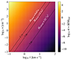 |
Fig. 1. Continuous color map of the parameter ṁ across a grid of characteristic velocities and hydrogen number densities considering a fixed PBH mass of 33 M⊙. The dashed black lines indicate the thresholds for MeADAF, MADAF, and MLHAF as a function of the viscosity parameter α = 0.1. The region above MLHAF corresponds to the thin-disk formation regime, while in the region between MLHAF and MADAF, LHAF occurs. The area between MADAF and MeADAF corresponds to the standard ADAF. The eADAF regime exists below MeADAF. |
Figure 2 displays examples of the resultant spectra (calculated using the formalism described above) generated by PBHs within varying gas density environments and having different masses, all at a fixed characteristic velocity in the medium of 10 km/s. The curves showing a knee are indicative of thin-disk emission. With higher densities at a certain PBH mass, the power produced by PBHs increases.
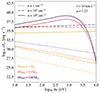 |
Fig. 2. Spectra generated by accreting PBHs of 1, 33, and 100 M⊙ (in yellow, red, and purple, respectively) in different gas density environments (1 cm−3 as dotted lines, 102 cm−3 as dash-dotted lines, and 104 cm−3 as solid lines). This example assumes a constant characteristic velocity |

3. Implementation
In this section, we provide an overview of our semianalytical model implementation. We start by introducing the hydrodynamical simulation we used and then describe the essential subgrid physics. Given our focus on implementing PBHs on galactic scales, where the dynamical and temporal timescales vary widely, we required simplifications and adaptations to mimic the expected effects at the scales we can resolve.
3.1. CIELO simulations
We worked with the high-resolution run of the CIELO suite of zoom-in hydrodynamical simulations. This project aimed to study the assembly and evolution of galaxies in different environments (Tissera in prep.; Rodríguez et al. 2022; Cataldi et al. 2023).
These simulations adopted a ΛCDM cosmology with Ω0 = 0.317, ΩΛ = 0.6825, ΩB = 0.049, and h = 0.6711 (Planck Collaboration I 2014).
The version of GADGET-3 we used to run these simulations includes a multiphase model for the gas component, metal-dependent cooling (Sutherland & Dopita 1993), star formation, and supernova (SN) feedback as described in Scannapieco et al. (2005) and Scannapieco et al. (2006). These multiphase and SN-feedback models were used to successfully reproduce the star formation activity of galaxies during quiescent and starburst phases and can drive violent mass-loaded galactic winds with a strength reflecting the depth of the potential well (Scannapieco et al. 2005, 2006). This physically motivated thermal SN-feedback scheme does not include any ad hoc mass-scale-dependent parameters. As a consequence, it is particularly well suited for the study of galaxy formation in a cosmological context.
For this work, we used the highest-resolution run of the Pehuen halos1 of the CIELO suite, which corresponds to 29 zoom-in initial conditions generated with the MUSIC code (Hahn & Abel 2011). Pehuen halos were taken from a DM-only run of a cosmological periodic cubic box with a side length of L = 50 Mpc h−1. In the highest-resolution run, the DM mass resolution was 1.36 × 10⁵ M⊙ h−1, and the initial gas particle mass was 2.1 × 10⁴ M⊙ h−1.
Virialized halos were identified by applying the friends-of-friends (FoF) algorithm (Davis et al. 1985), and the substructures within each dark matter halo were selected by using the SUBFIND code (Springel et al. 2001; Dolag et al. 2009). Figure 3 illustrates the projected distribution of hydrogen number density and temperature in the simulation at z ∼ 23. The location of the halos considered for this analysis is highlighted. These halos have more than 15 and 20 gas an dark matter particles, respectively.
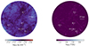 |
Fig. 3. Projected distribution of the hydrogen number density (left panel) and temperature (right panel) of gas in the Pehuen halos at z ∼ 23. Each halo considered in this paper is distinguished by a labeled circle with a radius equal to ten times the virial radius of the respective halo. |
Considering the nature of this work, it is relevant to mention that CIELO does not have a molecular cooling implementation, which is a relevant factor at the redshift under consideration. However, we applied this cooling semianalytically in post-processing to correctly follow the changes in the gas temperature due to PBHs at very high redshift. All physical processes were coded so that they could be switched off or on, as required.
The following sections provide a comprehensive description of the gas heating and cooling model (Sections 3.2 and 3.3, respectively), along with the application of these models to the simulation (Section 3.4). In this implementation, we considered each DM particle to consist of a specific constant fraction of PBHs (fPBH), and we assumed that the phase-space distribution of PBHs at the scales resolved by CIELO simulations is identical to that of standard cold DM. To select the gas particles affected by PBH feedback, for a DM particle i, we used the smoothed-particle hydrodynamics (SPH) smoothing length of the nearest gas particle, denoted as hi. Importantly, for the purposes of this paper, we chose to demonstrate the model outcomes at z ≈ 23, a time preceding the formation of the first stars in the simulation. This is because we do not expect PBH effects to be significant in comparison to SN feedback. Nonetheless, the versatility of our model extends to any other simulation and redshift.
3.2. Gas heating
We calculated the resulting heating power from the PBH emission as follows:
 (16)
(16)
where Lν(ν) is the specific luminosity at frequency ν, calculated using the formalism presented in Section 2.3. Here, fh is the fraction of energy deposited as heat. Following Takhistov et al. (2022), we adopted fh = 1/3, which is consistent with the estimates of Shull & van Steenberg (1985), Ricotti et al. (2002), Furlanetto & Stoever (2010), and Kim (2021). Additionally, τ is the optical depth for the gas component. The integral was computed over the energy range from Emin = 13.6 eV to Emax = 5Ti, with Ti as the characteristic temperature of the inner disk. For energies below Emin, hydrogen gas behaves as optically thin to continuous emission, leading to inefficient ionizing radiation absorption. Given the exponential decline of thin-disk emission spectra at higher energies, contributions beyond Emax become negligible.
For 13.6 eV < E < 30 eV, we employed the photoionization cross section given by (Bethe & Salpeter 1957; Band et al. 1990),
 (17)
(17)
where y = E/E0, E0 = 1/2Ei, and σ0 = 605.73 Mb = 6.06 × 10⁻¹⁶ cm2. Above 30 eV, we used attenuation length data from Figure (32.16) of Olive (2014).
The optical depth for a gas system of size l and with number density n is then given by
 (18)
(18)
3.3. Gas cooling
Since PBH feedback heats the surrounding gas, it is essential to correctly account for temperature loss due to cooling processes to determine the effective heating rate. In this section, we outline the cooling mechanisms we considered in our model.
3.3.1. Atomic cooling
We calculated the atomic cooling considering the processes described in Cen (1992), that is, collisional excitation of neutral hydrogen (H0) and singly ionized helium (He+) by electrons, collisional ionization of H0, He0, and He+, standard recombination of H+, He+, and He++, dielectronic recombination of He+, and free-free emission (bremsstrahlung) for all ions.
We adopted the cooling rates obtained by following the approach described in Katz et al. (1996), that is, considering collisional equilibrium abundances at any given temperature: The collisional excitation contributions from H and He dominate the cooling until the free–free transitions become important. Table 1 of Katz et al. (1996) contains the set of radiative cooling rates adopted in this work (the formulas were taken from Black 1981, with the modifications introduced by Cen 1992).
The atomic cooling functions we implemented are valid for gas temperatures higher than 5 × 10³ K. At temperatures outside this range, the formation of negative ions (H−) and molecules (H2,  ,
,  , and HeH+) can affect the thermal properties of the gas (Black 1981).
3.3.2. Molecular cooling
For gas temperatures lower than 5 × 10³ K, we considered molecular cooling by molecular hydrogen (H2) and hydrogen deuteride (HD). We implemented the H2 cooling following the model of Galli & Palla (1998). In this model, the final functional form of the total cooling in units of ergcm−3 s−1 is given by
 (19)
(19)
where ΛH2, LTE= HR + HV is the high-density limit, expressed as the sum of the rotational and the vibrational cooling at high densities, given by (Hollenbach & McKee 1979)
![Mathematical equation: $$ \begin{aligned} \begin{aligned} H_R=&\left(9.5 \times 10^{-22} T_3^{3.76}\right) /\left(1+0.12 T_3^{2.1}\right) \\&\times \exp \left[-\left(0.13 / T_3\right)^3\right]+3 \times 10^{-24} \exp \left[-0.51 / T_3\right] \\ H_V=\,&\, 6.7 \times 10^{-19} \exp \left(-5.86 / T_3\right) \\&+1.6 \times 10^{18} \exp \left(-11.7 / T_3\right) \end{aligned}, \end{aligned} $$](/articles/aa/full_html/2024/08/aa49650-24/aa49650-24-eq27.gif) (20)
(20)
with T3 = T/103, and ΛH2, n → 0 is the low-density limit, given by
![Mathematical equation: $$ \begin{aligned} \begin{aligned} \log \left(\Lambda _{\mathrm{H}_2, \mathrm{n} \rightarrow 0}\right)=\,&\, {\left[-103+97.59 \log (T)-48.05 \log (T)^2\right.} \\&\left.\times 10.8 \log (T)^3-0.9032 \log (T)^4\right] n_{\mathrm{H}}. \end{aligned} \end{aligned} $$](/articles/aa/full_html/2024/08/aa49650-24/aa49650-24-eq28.gif) (21)
(21)
The final H2 cooling is valid in the range 13 K < T < 105 K.
For HD cooling, we used the modified version of Lipovka et al. (2005) given by Coppola et al. (2011), which is valid for gas temperatures below 2 × 10⁴ K. Lipovka et al. (2005) provided a two-parameter fit of the collisional cooling function that depends on temperature and H fractional abundance. Coppola et al. (2011) evaluated a radiative cooling function that takes into account both dipole and quadrupole electric transitions, for which they used the calculations by Abgrall et al. (1982).
For completeness, we note that in primordial gas, another cooling agent is provided by LiH, but this is found to be always subdominant (Liu & Bromm 2018) and was thus not considered here.
3.3.3. Inverse-Compton cooling
In addition to the radiative cooling processes, we included IC cooling of the microwave background given by Ikeuchi & Ostriker (1986),
 (22)
(22)
where TCMB, z = 2.73 × (1 + z) is the CMB temperature at redshift z.
Finally, we took into account the volume expansion (contraction) of gas particles in each model iteration, resulting in adiabatic cooling (heating).
Given the heating and cooling theoretical framework, we describe below how we implemented them in our model.
3.4. Subgrid model
We worked with per-particle data extracted from the CIELO simulation, encompassing both gas and DM particles. Under the assumption that each DM particle contains a specific constant fraction of PBHs, we calculated the gas heating by PBH accretion over a period of 5 Myr starting at z = 22.85. This short period was chosen because it allowed us to assume that the particles did not undergo significant changes in their positions and were not strongly affected by gravitational effects among themselves. The starting redshift was chosen at the last available snapshot in the CIELO simulation before the onset of star formation. This setup allowed us to explore the possible impact of PBH feedback on gas properties, and hence, on the regulation of the star formation activity. Additionally, this also ensured that there were virialized halos containing at least ten gas particles. Given the substantial sensitivity of cooling rates to gas temperature, we executed gas heating and cooling computations through 135 discrete time steps. The selection of this time step count was determined through a convergence test that determined the minimum number of steps required for convergence while ensuring computational efficiency.
We recalculated the mass accreted by the PBHs at each time step by considering Eq. (1). We find that the mass accreted by PBHs is negligible in all our calculations, ensuring that the masses of the PBHs remains unchanged throughout the implementation.
Below, we provide a detailed breakdown of the iterative procedure steps.
-
We computed the density and characteristic velocity of the gas surrounding the PBHs. To accomplish this, we encompassed all gas particles within a sphere centered on a DM particle, with a radius equivalent to 2hi. The attributes of these gas particles were weighted using the spline kernel such that for a gas particle j (Monaghan & Lattanzio 1985),
 (23)
(23)where r represents the distance between DM particle i and gas particle j, and hj is the smoothing length of gas particle j. All properties were estimated by using the kernel to weight the contributions of the neighboring gas particles. These particles are called neighbors of a given DM particle.
-
We injected energy contributed by the PBHs associated with a given DM particle into all the gas neighbors of a given DM particle using the weights of Eq. (23).
-
After all the heating contributions resulting from accretion onto PBHs were incorporated into the thermal energy of each individual gas particle, we calculated the temperature increase and updated nH0, nH+, nHe0, nHe+, nHe++, and ne number densities using Eqs. (30)–(38) of Katz et al. (1996), but considering nH = nH0 + nH+ + nH2, with nH fixed at the value given by the CIELO simulation to conserve the numbers of hydrogen nuclei (see Appendix A for more details). For simplicity, nH2 was calculated by using the approximation of Tegmark et al. (1997), such that the fraction of H2 with respect to the total hydrogen number density was given by
 (24)
(24)This approximation is valid for gas temperatures T ≲ 103K, the temperature range in which cooling by H2 works.
-
Then, we cooled the gas depending on its temperature, as described in Sections 3.3.1, 3.3.2, and 3.3.3, and recalculated the per-particle gas volume due to adiabatic expansion or contraction.
3.5. Gas density treatment
Figure 3 shows that CIELO has resolution limitations that prevent us from considering the high densities expected at scales below 10 pc. To overcome this limitation in gas resolution, we adopted an innovative approach. We used the density profile at the onset of star formation, at z ≈ 30, within a halo of 2 × 10⁵ M⊙ from the case A zoom-in region for LCDM from Liu et al. (2022), which offers better resolution (hereafter referred to as the reference density profile). First, we rescaled the reference density profile so that it aligned with the virial mass of our halos. We achieved this by multiplying the reference profile by the ratio of the enclosed mass within our CIELO halos at their respective virial radii to the enclosed mass given by the reference halo at its virial radius. Although our implementation started at z ∼ 23, the mass of the reference density profile typically was within an order of magnitude of the masses of the halos present in CIELO. This effectively integrated the reference density profile into our simulations, compensating for resolution limitations below about 10 pc. Subsequently, by discerning the percentage of gas with a particular density within the halos, we determined the proportion of accretion inside the halo that occurred through each mechanism (eADAF, ADAF, LHAF, and thin disk), as these mechanisms are contingent upon the density of accreted gas. Figure 4 illustrates an example of the rescaled density profile for a CIELO halo (upper panel) and the enclosed mass profile (lower panel). With this information, we calculated in this example the accretion rate of a 33 M⊙ PBH using a mechanism determined by the gas density at different radial locations within the halo.
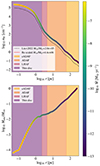 |
Fig. 4. Gas density profile and enclosed mass profile for a 33 M⊙ PBH. The upper panel displays the gas density profile taken from Liu et al. (2022) (dashed black line) alongside the rescaled density profile for one of our CIELO halos (red line). In the lower panel, the enclosed mass profile over the virial mass for this halo is shown. In both panels, the profiles are color-coded based on the gas-accretion rate of a 33 M⊙ PBH. For this particular example, we set |

We employed a subgrid model to characterize the density distribution of gas particles, focusing on the positions of neighboring gas surrounding DM particles. This method aids in identifying regions in which it is suitable to apply the halo density profile. To accomplish this, we employed a criterion that identifies halo-dominated regions when 70% of the neighboring gas particles are gravitationally bound to the halo. Following this, we used the rescaled reference density profile to the regions identified as halo-dominated.
This novel method successfully takes the gas density distributions within dark matter halos into account beyond the spatial scales that can be resolved in a cosmological context.
In Fig. 5, we present a comprehensive view of PBH accretion and heating across various masses (1 M⊙, 33 M⊙, and 100 M⊙ from left to right) within the density versus velocity plane. The contour lines delineate specific accretion regimes (eADAF, ADAF, and LHAF) that are aligned with the scheme in Fig. 1. The figure excludes the 10−12 M⊙ PBH case because the dominance of the eADAF regime across the entire velocity and density range for this mass leads to significantly lower accretion rates and heating values than for the other PBH masses explored in this study. All depicted results are representative of conditions at z ∼ 23, giving out the initial gas conditions in our implementation, hereafter referred to as the large-scale implementation.
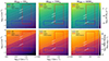 |
Fig. 5. Accretion and heating rates of PBHs with varying masses in the density vs. velocity plane. The color-coded panels illustrate the behavior of PBHs with varying masses (1 M⊙, 33 M⊙, and 100 M⊙ columns from left to right) in the density vs. velocity plane, depicting the accretion rate (upper row) and the resulting heating rate (bottom row). The dashed white lines delineate the upper limits of specific accretion regimes (eADAF, ADAF, and LHAF) as shown in Fig. 1. The red rectangles enclose the density and characteristic velocity ranges around each PBH within the halos, employing a rescaled version of the gas density profiles from Liu et al. (2022) and the CIELO particle velocities. The blue rectangles encapsulate weighted values around PBHs in the IGM. The dashed yellow line marks the peak density of a gas particle in the CIELO simulation. These results are representative of gas conditions at z ∼ 23. |
4. Results and discussion
4.1. Semianalytical model outcomes
This section presents our semianalytical model outcomes applied to the CIELO simulation, based on which, we explored the PBH impact on gas properties within and outside halos. The analysis took place at z ∼ 23 and the model was implemented over 5 Myr. We considered PBH masses of 1, 33, and 100 M⊙ as potential DM contributors. We also tested varied PBH DM contributions ranging from fPBH = 10−4 to 1. Our semianalytical model assessed changes in gas properties (in particular, nH, nH2, and T) for each PBH mass and fPBH combination.
As indicated in Eq. (1), the accretion rate depends not only on the gas density, but also on the mean molecular weight and on the characteristic velocity in the medium. Figure 6 presents a binned spatial distribution of DM particles surrounding a halo with a virial mass of 4.6 × 10⁶ M⊙ and a virial radius of 0.2 kpc. The color of each bin represents the average value of the relative velocity between the DM particle and the surrounding gas, the sound speed in the medium, and the mean molecular weight (from left to right). These properties distribution leads to different PBH accretion regimes and, consequently, different emission intensities. The characteristic velocity in the medium is primarily determined by the relative velocity between the gas and the DM particles.
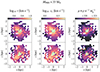 |
Fig. 6. Key gas properties around dark matter particles in projected spatial coordinates. The upper panels illustrate the spatially projected distribution of dark matter particles in the (x, y) coordinates, and the lower panels depict the distribution in the (x, z) coordinates. The colors indicate the mean values of the weighted (from left to right) relative velocity between the DM particle and the neighboring gas particles, the sound speed in the medium, and the mean molecular weight. The particle distribution is centered on a halo with Mvir = 4.6 × 10⁶ M⊙, Tvir = 8768 K, and rvir = 0.2 kpc, highlighted by cyan circles in each panel. |
In Fig. 7, the spatial distribution of gas particles is depicted, colored according to properties obtained through the implementation of our model. The left panel illustrates the ratio of the temperature when applying only our cooling model without PBH heating, and the virial temperature of the halo. The middle and right panel present results obtained by applying our reference model (MPBH, fPBH) = (33 M⊙, 1). In the middle panel, we show the ratio of the final temperature with this model and the virial temperature of the halo, and in the right panel, we display the final neutral hydrogen number density.
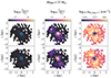 |
Fig. 7. As in Fig. 6, but for the spatial distribution of gas particles and the mean values (from left to right) of the ratio of the temperature obtained by applying only the cooling model (fPBH = 0) and the virial temperature of the halo, the ratio of the temperature considering the entire dark matter component as composed of 33 M⊙ PBHs (fPBH = 1) and the virial temperature of the halo (Tvir = 8768 K), and the final neutral gas density of this last model. |
The differences with and without PBHs are noticeable. While the gas can cool down in the cooling-only model (i.e., without the PBH model and only the cooling models), in the reference model, the gas experiences significant heating in regions with higher gas densities and lower characteristic velocities. Inside the halo, the temperature increases by roughly one order of magnitude compared to the virial temperature, and the neutral hydrogen gas density decreases considerably, rendering these conditions unsuitable for star formation.
We extended this analysis to six halos, covering a range of virial masses from 1.2 × 10⁶ to 4.7 × 10⁶ M⊙ and virial temperatures from 3800 K to 8800 K. We applied our implementation to all DM particles around approximately 14 × rvir, which was chosen to encompass gas particles well within the ISM and IGM.
In the bottom panels of Figs. 8 and 9, the medians of the final gas temperature and neutral hydrogen number density are displayed, respectively. These medians are presented as functions of the distance from the center of the halos. Initially, individual profiles were calculated for each halo, and subsequently, the median values were derived among the six halos. Each column corresponds to the results obtained considering different PBH masses and fPBH values. The middle and upper panels of Figs. 8 and 9 depict the ratios of the final temperature and neutral hydrogen number density values with and without PBHs, respectively. The upper panel of Fig. 8 shows the final gas temperature of the PBHs model over the virial temperature of the halo. For reference, the case with the cooling-only model implementation (fPBH = 0) is also included (yellow stars). The error bars represent the standard deviation within each distance bin.
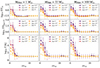 |
Fig. 8. Median temperature ratios and gas temperature as a function of distance from the halo center. From top to bottom, each row shows the median ratio of the final (i.e., after implementing our model) and the halo virial temperature, the median ratio of the final gas temperature and the gas temperature when only our cooling model is applied, and the median gas temperature. All as a function of distance from the halo center, expressed as a fraction of the virial radius. Each column from left to right corresponds to considering PBHs with masses of 1, 33, and 100 M⊙, with different fractions of DM composed of these PBHs, as indicated in each panel. For reference, we include the case of fPBH = 0, where we applied our cooling model alone. The error bars represent the standard deviation in each distance bin. Individual profiles were first calculated around each halo separately, and then the median values of the temperature ratios were derived from these individual profiles of the six halos. The virial temperatures range from 3800 to 8800 K. |
However, for higher PBH masses, an increase in PBH contributions to the DM budget, denoted by a higher value of fPBH, leads to more pronounced alterations in gas properties. Specifically, in the cases of PBH masses of 1 M⊙, 33 M⊙, and 100 M⊙, along with fractions exceeding or equal to 10−2, 10−3, and 10−3 respectively, the temperature rises to over 104 K, and the neutral hydrogen density is significantly affected toward the halo center. These changes in gas properties become less prominent at greater distances from the halo due to the properties of the medium (density and characteristic velocity), resulting in lower PBH accretion rates and, consequently, reduced energy injection into the medium. For this reason, our analysis was focused toward the halo center.
For a PBH mass of 1 M⊙, fractions of 10−2, 10−1, and 1 yield temperatures of (1.7, 2.0, and 2.0)Tvir, respectively, with these values representing the median within the halos. In terms of the temperature of the model without PBHs and employing our cooling model (TfPBH = 0) alone, these fractions result in temperatures toward the halo center of (324.8, 436.6, and 449.9)TfPBH = 0. Correspondingly, the neutral hydrogen density values as a fraction of the values considering our cooling implementation alone (nH0, fPBH = 0) are (2.3 × 10⁻³, 9.1 × 10⁻⁴, and 5.6 × 10⁻⁴)nH0, fPBH = 0.
For a 33 M⊙ PBH monochromatic mass function, varying fractions of 10−3, 10−2, 10−1, and 1 lead to temperatures proportional to (1.6, 1.9, 4.2, and 22.0)Tvir, respectively. In terms of TfPBH = 0, these fractions result in temperatures within regions near the halo center of (298.9, 407.2, 729.1, and 4949.4)TfPBH = 0. The corresponding neutral hydrogen density fractions are (2.7 × 10⁻³, 1.2 × 10⁻³, 1.0 × 10⁻⁵, and 2.0 × 10⁻⁹)nH0, fPBH = 0.
Similarly, for a 100 M⊙ PBH monochromatic mass function, fractions of 10−3, 10−2, 10−1, and 1 correspond to temperatures of (1.8, 2.2, 6.1, and 29.0)Tvir, respectively. In terms of TfPBH = 0, these fractions result in temperatures within regions near the halo center of (353.9, 460.0, 984.1, and 5847.6)TfPBH = 0. The corresponding neutral hydrogen density fractions are (1.9 × 10⁻³, 8.4 × 10⁻⁴, 1.2 × 10⁻⁶, and 1.4 × 10⁻⁹)nH0, fPBH = 0.
Our results indicate that the changes in temperature in the region closest to the halo center cause significant variations in the density of neutral hydrogen, which is crucial for the formation of molecular hydrogen and, consequently, for star formation. Due to the drastic alterations in gas properties, our findings suggest that PBHs with masses of 1 M⊙ and fractions greater than or equal to approximately 10−2 are ruled out. The same applies to PBHs with a mass of 33 M⊙ and 100 M⊙ and fractions greater than approximately 10−3. This is a more restricted limit than was found by Liu et al. (2022) for 33 M⊙ PBHs of 10−1.
It is noteworthy that the accretion rate depends on the mass of the PBH. Therefore, there are low PBH masses that do not produce any impact on the gas properties, and hence our method provides no constraints in these cases. We conducted a test using MPBH = 10−12 M⊙, a potential mass window for PBH DM. In this scenario, even if the entire DM component is composed of PBHs, the expected heating is negligible and is found not to affect the final gas temperature.
In a near future, we plan to carry out a new simulation that incorporates our model in a self-consistent way with the evolution of the gas component and subsequent stellar formation, which could provide insight into the effects of PBHs on the regulation of the transformation of gas into stars at the very early stages of galaxy formation.
4.2. Variations in the implementation
In addition to the results presented above, we explored alternative approaches in our implementation. This section summarizes our findings.
4.2.1. Energy injection
In addition to the standard SPH method for energy injection, we also tested a spherically symmetric radiative transfer approximation. This involved determining the mean free path as a function of photon energy from the accretion disk. Subsequently, we sorted all gas particles based on their distance to the PBH, and using an interpolated function for the photon energy as a function of the mean free path, we injected energy into each gas particle accordingly. While the computational cost of this method was significantly higher, the main trends observed remained consistent with our previous results.
4.2.2. Halo threshold
As described in Section 3.5, we used a particle selection criterion to identify halo-dominated regions. Regarding the application of the halo density profile, we assumed that the density profile is considered valid when 70% of particles around each DM particle reside within the halo. We also conducted tests using more conservative thresholds, such as 80%. However, due to the resolution limitations of our simulations, imposing a stricter limit often caused the profile to not being applied to the majority of halos. Consequently, this resulted in negligible temperature changes within the halos, even for a significant fraction of massive PBHs.
Notably, opting for lower limits frequently resulted in a substantial expansion of regions classified as ‘halo-dominated’, encompassing even areas far from the halo where the validity of the halo density profile is not expected. Specifically, for a 60% threshold for our halo sample, the count of DM particles encircled by a ‘halo-dominated’ region increased by as much as 50% to 400%, selecting 1.5 to 5 times the actual number of particles in the halo. This sensitivity emphasizes the importance of carefully setting this parameter to avoid overestimating the high-density regions.
4.2.3. Halo-scale analytical implementation
In this section, we study an alternative iteration of our implementation that was specifically crafted to solve the resolution challenge related to gas density in the cooling equations. It is important to note that although we employed the halo density profile from Liu et al. (2022) to calculate the heating rate of PBHs within halos, we refrained from adjusting the individual gas density of CIELO particles according to this profile. This decision was influenced by the mass resolution constraints inherent to these CIELO particles and also for the sake of simplicity. Consequently, the cooling rate in the higher-density regions within the halos might be underestimated.
To explore this limitation, we developed a fully analytical model at a halo scale. We used temperature and density data from Liu et al. (2022), as depicted in the upper panel of Fig. 10. To spatially distribute PBHs within the halo, we integrated a Navarro, Frenk, and White (NFW; Navarro et al. 1997) density profile. The lower panel of Fig. 10 illustrates the DM profile along with the distribution of PBHs at various radii based on their respective masses.
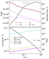 |
Fig. 10. Temperature, numerical densities, and DM density profiles as functions of distance from the halo center. In the upper panel, the continuous line illustrates the temperature (left y-axis), and the dashed lines represent numerical densities (right y-axis), both as functions of distance from the halo center in units of the virial radius, as obtained from Liu et al. (2022). In the lower panel, the continuous line denotes the DM density profile (NFW) on the left y-axis, and on the right y-axis, the number of PBHs enclosed within each radius for a specific monochromatic mass is shown, as labeled. The halo under consideration is at z = 30.3 and has Mvir = 2 × 10⁵ M⊙, with rvir = 60 pc. |
The method we adopted involves the creation of spherical shells within the halo, identifying regions with specific densities and temperatures. Instead of employing the SPH method, we employed the approach outlined in Section 4.2.1. The corresponding heating rates due to PBH accretion were calculated by using the same method as applied in our large-scale implementation and subsequently injected into each gas shell.
It is important to note that this model differs from the previous one in that it does not consider the energy contribution of gas heating due to accretion onto PBHs in the vicinity of the halo. This distinction may lead to an underestimation of heating. Additionally, a characteristic velocity of 10 km/s was fixed for the analysis, different from the previous implementation, where the characteristic velocity of CIELO particles was employed.
However, our primary focus was on cooling. Within this framework, the cooling rates were calculated by considering the high gas densities provided by the Liu et al. (2022) density profile.
The results illustrating the final gas temperature for a halo at z = 30.3, with a virial mass of Mvir = 2 × 10⁵ M⊙ and a virial radius of rvir = 60 pc are shown in Fig. 11. In regions of high density, close to the halo center, the temperature increase is generally more pronounced, peaking at densities near 103 cm−3. While high densities are considered in the cooling equations, it is observed that cooling does not surpass heating in the cases of interest. For instance, for MPBH = 1 M⊙ and fPBH = 10−4, the median temperature calculated using this implementation is 100 K, while the median temperature within the halo region depicted in Fig. 8 is 250 K.
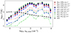 |
Fig. 11. Final gas temperature inside the halo characterized in Fig. 10 as a function of the initial neutral hydrogen number density of each gas shell. The final temperature is computed considering different PBHs masses and various fractions of DM composed of these PBHs, as labeled. The initial temperature is included with black circles. |
We also investigated the sensitivity of the results to variations in the virial halo masses, considering a range within the scale of CIELO halos. The observed trends in the final gas temperature remained consistent with our main results.
5. Summary and conclusions
We developed a semianalytical model that works on top of the CIELO hydrodynamical zoom-in simulation to investigate the influence of PBHs on gas properties within and outside halos at z ∼ 23. We comprehensively examined the evolution of gas properties, including temperature, molecular hydrogen density, and neutral hydrogen density, in the presence of PBHs around z ∼ 23. In the simulated region, we identified six halos with virial masses of about 106 M⊙.
We explored diverse combinations of PBH masses (1, 33, and 100 M⊙) and fractions of DM composed of these PBHs (10−4, 10−3, 10−2, 10−1, and 1). Our results revealed that PBHs with masses of 1 M⊙ and fractions greater than or equal to approximately 10−2 induce significant changes in gas properties. The same applies to PBHs with a mass of 33 M⊙ and 100 M⊙ and fractions greater than approximately 10−3. These alterations could potentially delay star-forming activities to lower redshifts than expected or might even inhibit star formation, particularly within the halos.
Notably, for 33 M⊙ PBHs with fractions exceeding 10−2, the final temperature increases by more than ten times compared to the initial temperature, and the neutral hydrogen density decreases to less than 10−3 times its initial value toward the halo center. Due to the temperature increase, the cooling time in this case is reduced by about ten times. Similar trends emerge with 100 M⊙ PBHs; a fraction exceeding approximately 10−3 leads to comparable variations in the gas properties to the latter PBH mass, however.
We further explored variations in our implementation, including a spherically symmetric radiative transfer calculation for energy injection. While this method exhibited consistent trends with our previous results, it was computationally more demanding. Additionally, we tested different particle selection criteria to consider a halo density profile. We found that setting the threshold at 70% yielded more applicable profiles for the thin-disk formation in halos with massive PBHs given our simulation resolution. On the other hand, more conservative thresholds, such as 80%, often resulted in negligible changes, underlining the sensitivity of the method to this parameter.
Moreover, we developed a fully analytical model based on an NFW profile and the gas density profile from Liu et al. (2022), allowing us to test the density treatment adopted in our semianalytical model.
In conclusion, our model implementation demonstrated significant variations in gas properties due to the presence of PBHs. Notably, PBHs with masses of 1 M⊙ and fractions greater than 10−2 markedly influence gas properties. This significant impact is also observed for PBHs with masses of 33 M⊙ and 100 M⊙ and fractions exceeding roughly 10−3. One important consideration is the potential influence of the Lyman-Werner radiation produced during PBH accretion, which could dissociate H2 and HD molecules. This process may result in less efficient cooling, and thus, in potentially higher final gas temperatures and more restrictive allowed fractions. This process will be analyzed in a future work.
A potential caveat regarding the temperature increase observed in our results is that the dynamical reaction of gas to PBH heating was not considered. When simulating heating or cooling and hydrodynamics on the fly, the feedback from PBHs can be self-regulated, so that strong accretion in dense regions will be rare. In this case, the heating by PBHs mostly operates at relatively low densities. When cooling wins at such low densities, the gas will collapse and form compact dense clumps. Some of these clumps may not contain PBHs and could still form stars, a phenomenon referred to as survivorship bias in Liu et al. (2022). In our case, we implicitly assumed that PBHs always exist in dense regions that can potentially form stars, which is not necessarily true in reality because of the discrete nature of PBHs and the self-regulation of BH accretion feedback, as shown in Liu et al. (2022). Moving forward, we aim to address this limitation by conducting self-consistent hydrodynamical simulations that incorporate the PBH accretion feedback model. This simulation will aim to validate our approach and offer deeper insights into the influence of PBHs on star formation processes.
Additionally, in the near future, our focus will be to use this PBH model to calculate the extensive radiation background generated by PBHs across X-ray and radio frequencies, employing semianalytical techniques. Furthermore, we plan to move away from assuming isotropic accretion by PBHs and instead consider the angular momentum of the accreted gas.
Despite the uncertainties in our idealized modeling, it is evident that the feedback exerted by PBHs on the primordial gas in the high-redshift Universe may lead to strong constraints on the properties of a possible PBH dark matter component. This thermal accretion-driven coupling with the gas fundamentally distinguishes PBH dark matter from the more standard particle-based alternatives, giving us an additional empirical probe to ascertain the nature of dark matter.
“Pehuen” is a term from Mapudungú used to refer to the Araucaria araucana tree, a native specie from South America found in Chile and Argentina. It is renowned for its edible pine nuts and has cultural significance among indigenous communities.
Acknowledgments
CC is supported by ANID-PFCHA/Doctorado Nacional/2020 – 21202137. PBT acknowledges partial funding by Fondecyt-ANID 1200703/2020, 1240465/2024, and ANID Basal Project FB210003. NDP was supported by a RAICES, a RAICES-Federal and PICT-2021-I-A-00700 grants from the Ministerio de Ciencia, Tecnología e Innovación, Argentina. BL is supported by the Royal Society University Research Fellowship. SP acknowledges partial support from MinCyT through BID PICT 2020 00582 and from CONICET through PIP 2022 0214 RDT thanks the Ministerio de Ciencia e Innovación (Spain) for financial support under Project grant PID2021-122603NB-C21. This project has received funding from the European Union Horizon 2020 Research and Innovation Programme under the Marie Sklodowska-Curie grant agreement No 734374- LACEGAL. We acknowledge the use of the Ladgerda Cluster (Fondecyt 1200703/2020). The numerical simulation is part of the CIELO project, was performed at the Barcelona Supercomputer Center.
References
- Abbott, B., Abbott, R., Abbott, T., et al. 2016, Phys. Rev. Lett., 116, 061102 [CrossRef] [PubMed] [Google Scholar]
- Abbott, R., Abbott, T. D., Abraham, S., et al. 2021, ApJ, 913, L7 [NASA ADS] [CrossRef] [Google Scholar]
- Abgrall, H., Roueff, E., & Viala, Y. 1982, A&AS, 50, 505 [NASA ADS] [Google Scholar]
- Agol, E., & Kamionkowski, M. 2002, MNRAS, 334, 553 [NASA ADS] [CrossRef] [Google Scholar]
- Araya, I. J., Rubio, M. E., San Martín, M., et al. 2021, MNRAS, 503, 4387 [NASA ADS] [CrossRef] [Google Scholar]
- Band, I. M., Trzhaskovskaia, M. B., Verner, D. A., & Iakovlev, D. G. 1990, A&A, 237, 267 [NASA ADS] [Google Scholar]
- Baudis, L. 2012, Phys. Dark Univ., 1, 94 [NASA ADS] [CrossRef] [Google Scholar]
- Bethe, H. A., & Salpeter, E. E. 1957, in Quantum Mechanics of One- and Two-Electron Systems (Berlin, Heidelberg: Springer), 88 [Google Scholar]
- Bird, S., Cholis, I., Muñoz, J. B., et al. 2016, Phys. Rev. Lett., 116, 201301 [NASA ADS] [CrossRef] [Google Scholar]
- Black, J. H. 1981, MNRAS, 197, 553 [NASA ADS] [Google Scholar]
- Boldrini, P., Miki, Y., Wagner, A. Y., et al. 2020, MNRAS, 492, 5218 [Google Scholar]
- Boveia, A., & Doglioni, C. 2018, Ann. Rev. Nucl. Part. Sci., 68, 429 [CrossRef] [Google Scholar]
- Carr, B. 2019, Astrophys. Space Sci. Proc., 56, 29 [NASA ADS] [CrossRef] [Google Scholar]
- Carr, B. J., & Rees, M. J. 1984, MNRAS, 206, 801 [NASA ADS] [CrossRef] [Google Scholar]
- Carr, B., & Silk, J. 2018, MNRAS, 478, 3756 [NASA ADS] [CrossRef] [Google Scholar]
- Carr, B., Kohri, K., Sendouda, Y., & Yokoyama, J. 2021, Rep. Prog. Phys., 84, 116902 [CrossRef] [Google Scholar]
- Cataldi, P., Pedrosa, S. E., Tissera, P. B., et al. 2023, MNRAS, 523, 1919 [NASA ADS] [CrossRef] [Google Scholar]
- Cen, R. 1992, ApJS, 78, 341 [NASA ADS] [CrossRef] [Google Scholar]
- Clesse, S., & García-Bellido, J. 2015, Phys. Rev. D, 92, 023524 [NASA ADS] [CrossRef] [Google Scholar]
- Clesse, S., & García-Bellido, J. 2017, Phys. Dark Univ., 15, 142 [NASA ADS] [CrossRef] [Google Scholar]
- Cole, P. S., & Byrnes, C. T. 2018, JCAP, 2018, 019 [CrossRef] [Google Scholar]
- Coppola, C. M., Lodi, L., & Tennyson, J. 2011, MNRAS, 415, 487 [NASA ADS] [CrossRef] [Google Scholar]
- Davis, M., Efstathiou, G., Frenk, C. S., & White, S. D. M. 1985, ApJ, 292, 371 [Google Scholar]
- Dolag, K., Borgani, S., Murante, G., & Springel, V. 2009, MNRAS, 399, 497 [Google Scholar]
- Feng, J. L. 2010, ARA&A, 48, 495 [NASA ADS] [CrossRef] [Google Scholar]
- Furlanetto, S. R., & Stoever, S. J. 2010, MNRAS, 404, 1869 [NASA ADS] [Google Scholar]
- Galli, D., & Palla, F. 1998, A&A, 335, 403 [NASA ADS] [Google Scholar]
- García-Bellido, J., & Ruiz Morales, E. 2017, Phys. Dark Univ., 18, 47 [CrossRef] [Google Scholar]
- Glazebrook, K., Nanayakkara, T., Schreiber, C., et al. 2024, Nature, 628, 277 [NASA ADS] [CrossRef] [Google Scholar]
- Gow, A. D., Byrnes, C. T., Cole, P. S., & Young, S. 2021, JCAP, 2021, 002 [Google Scholar]
- Green, A. M., & Kavanagh, B. J. 2021, J. Phys. G Nucl. Part. Phys., 48, 043001 [NASA ADS] [CrossRef] [Google Scholar]
- Hahn, O., & Abel, T. 2011, MNRAS, 415, 2101 [Google Scholar]
- Hawking, S. 1971, MNRAS, 152, 75 [Google Scholar]
- Hawkins, M. R. S. 2020, A&A, 643, A10 [NASA ADS] [CrossRef] [EDP Sciences] [Google Scholar]
- Hollenbach, D., & McKee, C. F. 1979, ApJS, 41, 555 [Google Scholar]
- Hopkins, P. F. 2015, MNRAS, 450, 53 [Google Scholar]
- Ikeuchi, S., & Ostriker, J. P. 1986, ApJ, 301, 522 [NASA ADS] [CrossRef] [Google Scholar]
- Kalaja, A., Bellomo, N., Bartolo, N., et al. 2019, JCAP, 2019, 031 [CrossRef] [Google Scholar]
- Kashlinsky, A. 2021, Phys. Rev. Lett., 126, 011101 [NASA ADS] [CrossRef] [Google Scholar]
- Kato, S., Fukue, J., & Mineshige, S. 2008, Black-Hole Accretion Disks– Towards a New Paradigm (Kyoto, Japan: Kyoto University Press), 549 [Google Scholar]
- Katz, N., Weinberg, D. H., & Hernquist, L. 1996, ApJS, 105, 19 [NASA ADS] [CrossRef] [Google Scholar]
- Kim, H. 2021, MNRAS, 504, 5475 [CrossRef] [Google Scholar]
- Labbé, I., van Dokkum, P., Nelson, E., et al. 2023, Nature, 616, 266 [CrossRef] [Google Scholar]
- Lipovka, A., Núñez-López, R., & Avila-Reese, V. 2005, MNRAS, 361, 850 [NASA ADS] [CrossRef] [Google Scholar]
- Liu, B., & Bromm, V. 2018, MNRAS, 476, 1826 [CrossRef] [Google Scholar]
- Liu, B., & Bromm, V. 2022, ApJ, 937, L30 [NASA ADS] [CrossRef] [Google Scholar]
- Liu, B., Zhang, S., & Bromm, V. 2022, MNRAS, 514, 2376 [NASA ADS] [CrossRef] [Google Scholar]
- MacGibbon, J. H. 1987, Nature, 329, 308 [NASA ADS] [CrossRef] [Google Scholar]
- Magaña, J., Martín, M. S., Sureda, J., et al. 2023, MNRAS, 520, 4276 [CrossRef] [Google Scholar]
- Mahadevan, R. 1997, ApJ, 477, 585 [NASA ADS] [CrossRef] [Google Scholar]
- Meszaros, P. 1975, A&A, 38, 5 [NASA ADS] [Google Scholar]
- Monaghan, J. J., & Lattanzio, J. C. 1985, A&A, 149, 135 [NASA ADS] [Google Scholar]
- Navarro, J. F., Frenk, C. S., & White, S. D. M. 1997, ApJ, 490, 493 [Google Scholar]
- Olive, K. 2014, Chin. Phys. C, 38, 090001 [Google Scholar]
- Padilla, N. D., Magaña, J., Sureda, J., & Araya, I. J. 2021, MNRAS, 504, 3139 [NASA ADS] [CrossRef] [Google Scholar]
- Page, D. N., & Hawking, S. W. 1976, ApJ, 206, 1 [NASA ADS] [CrossRef] [Google Scholar]
- Planck Collaboration I. 2014, A&A, 571, A1 [NASA ADS] [CrossRef] [EDP Sciences] [Google Scholar]
- Pringle, J. E. 1981, ARA&A, 19, 137 [NASA ADS] [CrossRef] [Google Scholar]
- Ricotti, M., Gnedin, N. Y., & Shull, J. M. 2002, ApJ, 575, 33 [NASA ADS] [CrossRef] [Google Scholar]
- Rodríguez, S., Garcia Lambas, D., Padilla, N. D., et al. 2022, MNRAS, 514, 6157 [CrossRef] [Google Scholar]
- Saito, R., Yokoyama, J., & Nagata, R. 2008, J. Cosmol. Astropart. Phys., 2008, 024 [CrossRef] [Google Scholar]
- Sasaki, M., Suyama, T., Tanaka, T., & Yokoyama, S. 2018, Phys. Rev. Lett., 121, 059901 [CrossRef] [Google Scholar]
- Sato-Polito, G., Kovetz, E. D., & Kamionkowski, M. 2019, Phys. Rev. D, 100, 063521 [NASA ADS] [CrossRef] [Google Scholar]
- Scannapieco, C., Tissera, P. B., White, S. D. M., & Springel, V. 2005, MNRAS, 364, 552 [NASA ADS] [CrossRef] [Google Scholar]
- Scannapieco, C., Tissera, P. B., White, S. D. M., & Springel, V. 2006, MNRAS, 371, 1125 [NASA ADS] [CrossRef] [Google Scholar]
- Shakura, N. I., & Sunyaev, R. A. 1973, A&A, 24, 337 [NASA ADS] [Google Scholar]
- Shull, J. M., & van Steenberg, M. E. 1985, ApJ, 298, 268 [NASA ADS] [CrossRef] [Google Scholar]
- Springel, V., White, S. D. M., Tormen, G., & Kauffmann, G. 2001, MNRAS, 328, 726 [Google Scholar]
- Sureda, J., Magaña, J., Araya, I. J., & Padilla, N. D. 2021, MNRAS, 507, 4804 [CrossRef] [Google Scholar]
- Sutherland, R. S., & Dopita, M. A. 1993, ApJS, 88, 253 [Google Scholar]
- Takhistov, V., Lu, P., Gelmini, G. B., et al. 2022, J. Cosmol. Astropart. Phys., 2022, 017 [CrossRef] [Google Scholar]
- Tegmark, M., Silk, J., Rees, M. J., et al. 1997, ApJ, 474, 1 [NASA ADS] [CrossRef] [Google Scholar]
- Villanueva-Domingo, P., Mena, O., & Palomares-Ruiz, S. 2021, Front. Astron. Space Sci., 8, 681084 [CrossRef] [Google Scholar]
- Volonteri, M. 2010, A&ARv., 18, 279 [NASA ADS] [CrossRef] [Google Scholar]
- Yuan, F., & Narayan, R. 2014, ARA&A, 52, 529 [NASA ADS] [CrossRef] [Google Scholar]
- Zhang, S., Liu, B., & Bromm, V. 2024, MNRAS, 528, 180 [CrossRef] [Google Scholar]
- Ziparo, F., Gallerani, S., Ferrara, A., & Vito, F. 2022, MNRAS, 517, 1086 [NASA ADS] [CrossRef] [Google Scholar]
- Zwicky, F. 1933, Helvetica Phys. Acta, 6, 110 [NASA ADS] [Google Scholar]
Appendix A: Chemistry in the model
For a specified density, temperature, and ionizing background spectrum, we used the slightly modified equations from Katz et al. (1996), accounting for the presence of H2, to determine the values of nH0, nH+, nHe0, nHe+, nHe++, and ne,
 (A.1)
(A.1)
 (A.2)
(A.2)
 (A.3)
(A.3)
 (A.4)
(A.4)
 (A.5)
(A.5)
 (A.6)
(A.6)
where y = (nHe0 + nHe+ + nHe++)/nH, and we assumed ΓγHe0 = ΓγHe+ = 0.
The collisional ionization rates (ΓeH0, etc.) and recombination rates (αH+, etc.) are listed in in Table A.1.
Recombination and collisional ionization rates
All Tables
All Figures
|
Fig. 1. Continuous color map of the parameter ṁ across a grid of characteristic velocities and hydrogen number densities considering a fixed PBH mass of 33 M⊙. The dashed black lines indicate the thresholds for MeADAF, MADAF, and MLHAF as a function of the viscosity parameter α = 0.1. The region above MLHAF corresponds to the thin-disk formation regime, while in the region between MLHAF and MADAF, LHAF occurs. The area between MADAF and MeADAF corresponds to the standard ADAF. The eADAF regime exists below MeADAF. |
| In the text | |
|
Fig. 2. Spectra generated by accreting PBHs of 1, 33, and 100 M⊙ (in yellow, red, and purple, respectively) in different gas density environments (1 cm−3 as dotted lines, 102 cm−3 as dash-dotted lines, and 104 cm−3 as solid lines). This example assumes a constant characteristic velocity |
| In the text | |
|
Fig. 3. Projected distribution of the hydrogen number density (left panel) and temperature (right panel) of gas in the Pehuen halos at z ∼ 23. Each halo considered in this paper is distinguished by a labeled circle with a radius equal to ten times the virial radius of the respective halo. |
| In the text | |
|
Fig. 4. Gas density profile and enclosed mass profile for a 33 M⊙ PBH. The upper panel displays the gas density profile taken from Liu et al. (2022) (dashed black line) alongside the rescaled density profile for one of our CIELO halos (red line). In the lower panel, the enclosed mass profile over the virial mass for this halo is shown. In both panels, the profiles are color-coded based on the gas-accretion rate of a 33 M⊙ PBH. For this particular example, we set |
| In the text | |
|
Fig. 5. Accretion and heating rates of PBHs with varying masses in the density vs. velocity plane. The color-coded panels illustrate the behavior of PBHs with varying masses (1 M⊙, 33 M⊙, and 100 M⊙ columns from left to right) in the density vs. velocity plane, depicting the accretion rate (upper row) and the resulting heating rate (bottom row). The dashed white lines delineate the upper limits of specific accretion regimes (eADAF, ADAF, and LHAF) as shown in Fig. 1. The red rectangles enclose the density and characteristic velocity ranges around each PBH within the halos, employing a rescaled version of the gas density profiles from Liu et al. (2022) and the CIELO particle velocities. The blue rectangles encapsulate weighted values around PBHs in the IGM. The dashed yellow line marks the peak density of a gas particle in the CIELO simulation. These results are representative of gas conditions at z ∼ 23. |
| In the text | |
|
Fig. 6. Key gas properties around dark matter particles in projected spatial coordinates. The upper panels illustrate the spatially projected distribution of dark matter particles in the (x, y) coordinates, and the lower panels depict the distribution in the (x, z) coordinates. The colors indicate the mean values of the weighted (from left to right) relative velocity between the DM particle and the neighboring gas particles, the sound speed in the medium, and the mean molecular weight. The particle distribution is centered on a halo with Mvir = 4.6 × 10⁶ M⊙, Tvir = 8768 K, and rvir = 0.2 kpc, highlighted by cyan circles in each panel. |
| In the text | |
|
Fig. 7. As in Fig. 6, but for the spatial distribution of gas particles and the mean values (from left to right) of the ratio of the temperature obtained by applying only the cooling model (fPBH = 0) and the virial temperature of the halo, the ratio of the temperature considering the entire dark matter component as composed of 33 M⊙ PBHs (fPBH = 1) and the virial temperature of the halo (Tvir = 8768 K), and the final neutral gas density of this last model. |
| In the text | |
|
Fig. 8. Median temperature ratios and gas temperature as a function of distance from the halo center. From top to bottom, each row shows the median ratio of the final (i.e., after implementing our model) and the halo virial temperature, the median ratio of the final gas temperature and the gas temperature when only our cooling model is applied, and the median gas temperature. All as a function of distance from the halo center, expressed as a fraction of the virial radius. Each column from left to right corresponds to considering PBHs with masses of 1, 33, and 100 M⊙, with different fractions of DM composed of these PBHs, as indicated in each panel. For reference, we include the case of fPBH = 0, where we applied our cooling model alone. The error bars represent the standard deviation in each distance bin. Individual profiles were first calculated around each halo separately, and then the median values of the temperature ratios were derived from these individual profiles of the six halos. The virial temperatures range from 3800 to 8800 K. |
| In the text | |
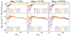 |
Fig. 9. Same as the middle and lower panels of Fig. 8, but for the neutral hydrogen number density. |
| In the text | |
|
Fig. 10. Temperature, numerical densities, and DM density profiles as functions of distance from the halo center. In the upper panel, the continuous line illustrates the temperature (left y-axis), and the dashed lines represent numerical densities (right y-axis), both as functions of distance from the halo center in units of the virial radius, as obtained from Liu et al. (2022). In the lower panel, the continuous line denotes the DM density profile (NFW) on the left y-axis, and on the right y-axis, the number of PBHs enclosed within each radius for a specific monochromatic mass is shown, as labeled. The halo under consideration is at z = 30.3 and has Mvir = 2 × 10⁵ M⊙, with rvir = 60 pc. |
| In the text | |
|
Fig. 11. Final gas temperature inside the halo characterized in Fig. 10 as a function of the initial neutral hydrogen number density of each gas shell. The final temperature is computed considering different PBHs masses and various fractions of DM composed of these PBHs, as labeled. The initial temperature is included with black circles. |
| In the text | |
Current usage metrics show cumulative count of Article Views (full-text article views including HTML views, PDF and ePub downloads, according to the available data) and Abstracts Views on Vision4Press platform.
Data correspond to usage on the plateform after 2015. The current usage metrics is available 48-96 hours after online publication and is updated daily on week days.
Initial download of the metrics may take a while.