| Issue |
A&A
Volume 697, May 2025
|
|
|---|---|---|
| Article Number | A65 | |
| Number of page(s) | 10 | |
| Section | Extragalactic astronomy | |
| DOI | https://doi.org/10.1051/0004-6361/202553701 | |
| Published online | 07 May 2025 | |
Can primordial black holes explain the overabundance of bright super-early galaxies?
1
Scuola Normale Superiore, Piazza dei Cavalieri 7, 56126 Pisa, Italy
2
Dipartimento di Fisica “Enrico Fermi”, Università di Pisa, Largo Bruno Pontecorvo 3, Pisa I-56127, Italy
⋆ Corresponding author.
Received:
8
January
2025
Accepted:
26
February
2025
Abstract
The James Webb Space Telescope (JWST) is detecting an excess of high-redshift (z ≳ 10) bright galaxies that challenge most theoretical predictions. To address this issue, we investigated the impact of primordial black holes (PBHs) on the halo mass function and UV luminosity function (LF) of super-early galaxies. We explored two key effects: (i) The enhancement of the massive halo abundance due to the compact nature and spatial distribution of PBHs, and (ii) the luminosity boost, characterized by the Eddington ratio λE, caused by active galactic nuclei (AGN) that are powered by matter accretion onto PBHs. We built an effective model, calibrated using data at lower redshifts (z ≈ 4 − 9), to derive the evolution of the LF, including the additional PBH contribution. A Bayesian analysis yielded the following results: (a) Although a small fraction (log fPBH ≈ −5.42) of massive (log MPBH/M⊙ ≈ 8.37) nonemitting (λE = 0) PBHs can explain the galaxy excess via the halo abundance enhancement, this solution is excluded by cosmic microwave background μ-distortion constraints on monochromatic PBHs. (b) If PBHs power an AGN that emits at super-Eddington luminosity (λE ≈ 10), the observed LF can be reproduced by a PBH population with a characteristic mass log MPBH/M⊙ ≈ 3.69, constituting a tiny (log fPBH ≈ −8.16) fraction of the cosmic dark matter content. In the AGN scenario, about 75% of the observed galaxies with MUV = −21 at z = 11 should host a PBH-powered AGN and typically reside in low-mass halos, Mh = 108 − 9 M⊙. These predictions can be tested with available and forthcoming JWST spectroscopic data. We note that our analysis considered a lognormal PBH mass function and compared its parameters with monochromatic limits on the PBH abundance. Further work is required to relax these limitations.
Key words: galaxies: evolution / galaxies: high-redshift / galaxies: luminosity function / mass function / quasars: supermassive black holes
© The Authors 2025
 Open Access article, published by EDP Sciences, under the terms of the Creative Commons Attribution License (https://creativecommons.org/licenses/by/4.0), which permits unrestricted use, distribution, and reproduction in any medium, provided the original work is properly cited.
This article is published in open access under the Subscribe to Open model. This email address is being protected from spambots. You need JavaScript enabled to view it. to support open access publication.
1. Introduction
Since its launch, the James Webb Space Telescope (JWST) led to the photometric discovery (Naidu et al. 2022; Castellano et al. 2022; Atek et al. 2023; Labbé et al. 2023) and spectroscopical analysis (Arrabal Haro et al. 2023; Bunker et al. 2023; Curtis-Lake et al. 2023; Robertson et al. 2023; Wang et al. 2023; Hsiao et al. 2024; Zavala et al. 2025) of galaxies up to about redshift z = 14 (Carniani et al. 2024), when the Universe was ≈300 Myr old. The abundant new data from the JWST shed light on the primordial Universe. This allows us to study the first galaxies in great detail. The analysis of the observations has shown an excess of high-redshift (z ≳ 10) bright galaxies that challenge most theoretical predictions (Labbé et al. 2023; Robertson et al. 2023, 2024; Casey et al. 2024; Harvey et al. 2025; Finkelstein et al. 2024; Fujimoto et al. 2024).
The inferred abundance of these systems is indeed higher by about an order of magnitude than any prediction based on pre-JWST data, such as hydrodynamical simulations (e.g., IllustrisTNG, Vogelsberger et al. 2020; FLARES, Vijayan et al. 2021; BlueTides, Wilkins et al. 2017), abundance-matching models (e.g., UniverseMachine, Behroozi et al. 2020), and also extrapolations from lower-redshift fits (e.g. Bouwens et al. 2022a) of the ultraviolet (UV) luminosity function (LF). This tension constitutes an important challenge to our knowledge of the galaxy formation and evolution process in the early Universe, and several possible solutions have been proposed to solve this problem.
Astrophysical solutions include a stochastic star formation rate (SFR) in early galaxies that could boost the bright end of the LF to the observed level (Mason et al. 2023; Shen et al. 2024). However, (i) the magnitude of the SFR flickering predicted from simulations is debated (Pallottini & Ferrara 2023; Sun et al. 2023), (ii) the rms amplitude necessary to explain the overabundance problem was shown to be inconsistent with the observed mass-metallicity relation (Pallottini et al. 2024), and (iii) an analysis of the spectral energy density showed that the SFR stochasticity of early galaxies is relatively low (Ciesla et al. 2024).
Alternatively, the tension can be solved by scenarios in which either a negligible dust attenuation produced by radiation-driven outflows brightens the galaxies (attenuation-free, Ferrara et al. 2023, 2025), or the star formation efficiency is high due to inefficient supernova feedback in dense regions (Dekel et al. 2023). These models and their implications are still under scrutiny.
Moreover, modifications of the “concordance” Λ cold dark matter (ΛCDM) model have also been explored. If the number density of massive halos were indeed higher than predicted by ΛCDM, the tension could be released without postulating significant changes in the underlying astrophysics (e.g., star formation efficiency or dust attenuation). This can be achieved, for instance, by assuming different cosmological scenarios, such as an early dark energy contribution at z ≈ 3500 (Klypin et al. 2021); shen:2024 that significantly changes the halo abundance at z > 10. In addition, the halo mass function (HMF) can also be enhanced (i) by an effective modification of the transfer function (Padmanabhan & Loeb 2023), (ii) by non-Gaussianities that make overdense regions more frequent (Biagetti et al. 2023), or (iii) by the contribution of primordial black holes (PBHs) to the halo formation (Liu & Bromm 2022).
However, these proposals might cause other tensions: (i) An enhanced transfer function is argued to be excluded by low-z Hubble observations (Sabti et al. 2024), (ii) the amplitude of non-Gaussian fluctuations is tightly constrained by cosmic microwave background (CMB) observations (Planck Collaboration IX 2020), and (iii) a monochromatic ≈1010 M⊙ PBH solution contributing to structure formation is excluded by CMB μ-distortions (Chluba et al. 2012; Nakama et al. 2018; Gouttenoire et al. 2024).
We focus on the effects of PBHs on the observed galaxy LF by relaxing the constraints imposed by Liu & Bromm (2022) by considering the possibility that PBHs have an extended mass function, as predicted by some inflationary models (García-Bellido et al. 2021; Carr et al. 2021a), and/or non-negligibly contribute to the UV luminosity of the host galaxy. These two additions make the model more realistic and in principle allow lower-mass PBHs to affect observations without violating current CMB constraints (for the μ-distortion limit in particular, see Wang et al. 2025)1.
2. Methods
We started by fixing the astrophysical model for star formation, emission, and attenuation by matching low-redshift (z ≈ 4 − 9) data before considering the potential effects of PBHs. To do this, we computed the HMF for a given PBH mass distribution (Sect. 2.1), fit the stellar emission of galaxies to the low-z LF (Sect. 2.2), added the PBH emission contribution to the total UV luminosity (Sect. 2.3), computed the theoretical LF when PBHs are present (Sect. 2.4), and then determined the main parameters within a Bayesian framework (Sect. 2.5).
2.1. PBH effects on the structure formation
Following Inman & Ali-Haïmoud (2019), the power spectrum of ΛCDM can be modified through an additional term to account for the Poissonian shot noise (Carr & Silk 2018) produced by the discrete nature of PBHs,
 (1a)
(1a)
with
 (1b)
(1b)
where nPBH is the comoving number density of PBHs, D = D(z) is the growth factor2 from Inman & Ali-Haïmoud (2019), and fPBH can be written as
 (1c)
(1c)
for a monochromatic mass function. Θ is the step function that suppresses the PBH contribution on scales smaller than the critical one (Liu & Bromm 2022)
 (1d)
(1d)
These scales are strongly affected by nonlinear evolution through the seed effect (Carr & Silk 2018) and by mode mixing between isocurvature and adiabatic modes (Liu et al. 2022). We normalized the power spectrum in Eq. (1) by imposing the value for σ(R = 8 h−1 Mpc) = σ8 from Planck Collaboration VI (2020).
Following the excursion set theory for the halo collapse and using the approach from Press & Schechter (1974) accounting for the ellipsoidal collapse (Sheth & Tormen 2002), we computed the comoving number density of dark matter halos (halo mass function; HMF) as a function of z and of the halo mass (Mh).
Eq. (1) hold for PBHs with a monochromatic mass function, as considered by Liu & Bromm (2022). We allowed PBHs to have an extended mass function and adopted a lognormal distribution,
![Mathematical equation: $$ \begin{aligned} \dfrac{\mathrm{d} n({>}M)}{\mathrm{d} \log M} \propto \frac{1}{\sqrt{2\pi }\sigma } \exp \left[-\frac{1}{2}\left(\frac{\log M/M_{\rm PBH}}{\sigma }\right)^2\right], \end{aligned} $$](/articles/aa/full_html/2025/05/aa53701-25/aa53701-25-eq5.gif) (2)
(2)
where MPBH is the characteristic mass of PBHs, and σ is the rms of the distribution; the constant of proportionality was fixed by normalizing the integral of the distribution to fPBH. The monochromatic case can be retrieved in the limit σ → 0.
The lognormal mass function for PBHs is predicted by several inflationary models (e.g. Dolgov & Silk 1993; Green 2016; Kannike et al. 2017), and we chose it for its simple analytical form with only three parameters. Other mass functions are produced when considering different models (e.g. García-Bellido et al. 2021), eventually spanning a wider mass range than the lognormal and/or having several peaks. Further investigation should be undertaken to test them within our framework.
In Fig. 1 we show the HMF at z = 11 for several PBH models to highlight the differences to the standard ΛCDM structure formation. The corresponding power spectra are shown in the inset. Although in this case, PBHs constitute only a small fraction fPBH = 10−5 of the dark matter density, they can significantly affect the power spectrum with a boost of ≈10× around kcrit. The width of the mass function changes the sharpness of the power spectrum contribution, that is, the higher σ, the smoother it is around kcrit. An important feature of the power spectrum is the bump shift toward lower k for higher σ values. This is caused by the extended tail of the lognormal distribution. The general effect on the HMF is an enhancement in the halo abundance on a wide mass range that peaks at a mass scale slightly higher than MPBH. More massive PBHs require a smaller fPBH to imprint the same relative increase in the halo abundance around MPBH.
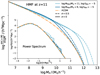 |
Fig. 1. Overview of the modifications to the HMF due to the PBH contribution to the power spectrum. The Sheth & Tormen (2002) HMF (n) at z = 11 is plotted as a function of halo mass (Mh) for a pure ΛCDM cosmology and for PBHs with lognormal mass functions, constituting a fraction fPBH = 10−5 of the total dark matter density; each color corresponds to a different PBH mass MPBH = 109 M⊙, 1011 M⊙, whereas continuous (dashed) lines represent monochromatic (lognormal with σ = 0.5) mass functions. For reference, we show the corresponding power spectra at z = 0 (PCDM, Eq. 1) as a function of the wavenumber (k) as an inset. |
The extended mass function changes the functional form of the power spectrum term in Eq. (1b), which must now be replaced with that in Eq. (A.5). In particular, the Θ function becomes smoother and has a width that depends on σ; the explicit derivation is given in Appendix A.
2.2. Stellar emission
We built an effective model for the stellar emission from galaxies that matched pre-JWST LF data and set our baseline for super-early galaxy applications. The LF (ΦUV) as a function of z was computed from the halo mass function n(> Mh, z) through the chain rule
 (3)
(3)
where Mh is the mass of halos hosting galaxies of magnitude MUV. With this approach, we only need an emission model MUV = MUV(Mh, z), that is, the expected magnitude of a galaxy based on its halo mass. This implicitly neglects possible stochasticity contributions to the galaxy emission (see e.g. Mason et al. 2023; Pallottini & Ferrara 2023; Gelli et al. 2024; Sun et al. 2024, for more details on the impact).
We chose a flexible functional form for the emission model,
![Mathematical equation: $$ \begin{aligned} M_{\rm UV} = p_1 + \left[p_2 \left(\frac{M_{\rm h}}{10^{11}\,\mathrm{M_\odot }}\right)^{p_3} + p_4\right] \log \left(\frac{M_{\rm h}}{10^{11}\,\mathrm{M_\odot }}\right) + p_5 z^{p_6} \end{aligned} $$](/articles/aa/full_html/2025/05/aa53701-25/aa53701-25-eq7.gif) (4)
(4)
where pi are parameters. The function combines a power law with a logarithm to properly match the LF at a fixed redshift with an additional term for the explicit dependence on z. Although this particular choice lacks a clear physical motivation, we find that it gives good results over the whole redshift range we considered. We fit these parameters to the LF data at z = 4, 5, 6, 7, 8, and 9 from Bouwens et al. (2021) by assuming a purely ΛCDM model (fPBH = 0 in Eq. 1) when computing the LF (Eq. 3). The errors on LF data were treated as Gaussian, which is a rough approximation, but allowed us to account for uncertainties in the fit in a simple way. The result is given by
 (5)
(5)
where the error of the fit is relatively large because of the strong correlation between the parameters retrieved from the six-parameter least-squares error procedure.
In Fig. 2 we report the modeled LF at different z along with the fitting data (Bouwens et al. 2021) and the Schechter function fit3 from Bouwens et al. (2022a). The fitting function (Eq. 4) appears to provide a very good approximation to the data over the whole redshift range of interest. The plot was produced using the best-fit values from Eq. (5) and neglecting their uncertainties. In general, this is a poor practice because it does not provide information about the robustness of the results. However, in this context, we are not interested in the precise values of the parameters, but only in the model agreement with the data points. In other words, it is not a problem if the solution we find does not have tightly constrained parameters. Therefore, we proceeded to neglect the uncertainties in Eq. (5) and considered only the best-fit values in the following treatment.
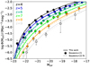 |
Fig. 2. Ultraviolet luminosity function of galaxies (Φ) at different redshifts compared to data (Bouwens et al. 2021, 2022a). The LF from our model (solid line, Eq. 4) was fit to the points at the reported redshifts (parameters in Eq. 5). |
We plot the MUV − Mh relation at z = 9 (Fig. 3) to compare our fiducial model with previous works. The models from Ferrara et al. (2023) were built through a semi-analytical model obtained by fitting the LF at z = 7 and considering the dust attenuation (Inami et al. 2022) from the REBELS survey (Bouwens et al. 2022b); in addition, the attenuation-free case is reported labeled AF. The model of Behroozi et al. (2019) used the stellar halo mass relation, which is derived via abundance matching, combined with their Eq. (D.5) to link the stellar mass to the UV magnitude, including dust attenuation. We also report the results of the BlueTides (Wilkins et al. 2017; Feng et al. 2015, 2016) hydrodynamical N-body simulation focused on the properties of galaxies with stellar masses M* ≥ 108 M⊙ at z ≥ 8. To compute the observed UV luminosity from simulated data, they assumed the intrinsic UV luminosity of a galaxy to be ∝SFR, and its dust attenuation to scale linearly with metallicity.
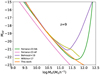 |
Fig. 3. Ultraviolet magnitude (MUV) as a function of Mh at z = 9 within different models. The relation in this work is obtained via a fit of the LF (see Eq. 4 for the functional form and Eq. 5 for the parameters). For comparison, we report MUV(Mh) from the semi-analytical model of Ferrara et al. (2023, in the dust-attenuated, DA, and attenuation-free, AF, cases), from the abundance-matching based procedure of Behroozi et al. (2019) and results from the BlueTides hydrodynamical simulations (Wilkins et al. 2017). |
Except for the attenuation-free case from Ferrara et al. (2023), the MUV − Mh relation from our model is very close to those from the literature up to Mh ≈ 1011 M⊙. Above this threshold, the models behave differently, and in our case, the luminosity of a galaxy monotonically increases with halo mass. This indicates that we may be missing heavily dust-obscured galaxies (expected in dust-attenuated models; see Ferrara et al. 2023 (DA), and Behroozi et al. 2019) and possibly also active galactic nucleus (AGN) feedback (considered in Wilkins et al. 2017). These effects become important only for MUV ≲ −22 and hence, they do not dramatically impact our conclusions.
We underline that we lack detailed information on the galaxy obscuration since it is included implicitly in the fit made with Eq. (4) (cf. with Ferrara et al. 2023). Fig. 3 shows that dust extinction affects only galaxies contained in massive (≳1012 M⊙), and thus rare, halos. We treat the AGN dust extinction in the following section.
2.3. PBH emission
An accreting PBH can emit light as AGN, and it can thus increase the brightness of its host galaxy. We quantified the PBH emission via the Eddington ratio λE, which is defined as the ratio of the AGN bolometric luminosity, Lbol, and its Eddington luminosity,
 (6)
(6)
where G is Newton’s constant, mp is the proton mass, c is the speed of light, and σT is the cross section for Thomson scattering. From the bolometric luminosity (Lbol = λELE), we retrieved the UV luminosity through the conversion factors from Shen et al. (2020)
 (7a)
(7a)
where
 (7b)
(7b)
and summed it to the stellar contribution to obtain the total emission from the galaxy,
 (7c)
(7c)
We did not explicitly account for dust attenuation in the AGN term, which reduces the observed luminosity, but considered it implicitly in the bolometric correction factors. The total UV magnitude was used to compute the LF including PBH emission. For simplicity, we assumed that λE is the same for each PBH, although more realistically, we do expect this parameter to have a wide distribution (Bhatt et al. 2024). The case in which PBHs do not emit can be retrieved by imposing λE = 0.
We caution that we used the same PBH mass function to compute the modified power spectrum and the PBH emission term, even though they should correspond to the spectra at matter-radiation equality and at the observed z, respectively. Stated differently, we neglected the accretion of PBHs from their formation epoch up to the observed z (Jangra et al. 2024; Nayak & Jamil 2012). This implies that the required λE values to fit the observed LF must be seen as upper limits. Assuming a specific model for accretion (e.g. Hasinger 2020), we can compute the PBH mass growth. Supposing that each of them grows by a factor K before z = 11, we retrieved the same results as considering a model in which PBH do not grow and setting  (further discussion in Sect. 4).
We underline that we did not account for the AGN duty cycle. Values < 1 for this quantity would reduce the number of active AGN, thus requiring a higher number of PBHs (i.e., fPBH) to retain the same results.
2.4. PBH spatial distribution
To properly estimate the contribution to the LF, we must populate galaxies with PBHs using some educated guesses.
First, we assumed that all PBHs reside in galactic halos rather than in the intergalactic medium. This choice maximized the impact of PBH emission at fixed fPBH and was motivated by the notion that PBHs may foster the growth of baryonic structures around them. This point has been made by some works, such as Inman & Ali-Haïmoud (2019, who conclude that isolated PBH are an artifact preferentially appearing for large fPBH values), while other works considered the presence of some intergalactic PBHs (Manzoni et al. 2024; Jangra et al. 2024).
Next, we distributed PBHs in halos with a mass Mh > Mmin = 107.5 M⊙. This choice was motivated by the fact that PBHs are probably not found in small halos and that galaxies hosted by halos with Mh < Mmin are fainter than the lowest LF constraints (according to our astrophysical model, Sect. 2.2). With higher Mmin values, the LF at z = 11 can instead not be reproduced properly by varying the model parameters because the predicted LF behaves differently at the faint end than the data. Our recipe is admittedly rough and should be refined based on more stringent physical arguments in the future. This could be done along the lines initially explored in Inman & Ali-Haïmoud (2019) and Liu et al. (2022).
In practice, we implemented the previous assumption by imposing that halos with Mh > Mmin contained a number of PBHs drawn from a Poisson distribution with mean x, independent of Mh. Each PBH was assigned a mass by extracting from the mass function. The value of x can be determined by matching the total cosmic number density of PBHs,
 (8)
(8)
where ⟨MPBH⟩ is the mass-function-averaged PBH mass, and n(> Mmin) is the number density of halos with Mh > Mmin. Therefore, we split the halos with a certain mass into groups based on the number of PBHs they host, we computed the PBH UV luminosity distribution within each group, and we added it to the stellar luminosity distribution. We finally binned the galaxies based on their UV luminosity to retrieve the LF. With this approach, halos of the same mass may host objects with different MUV due to the different contributions of PBHs, which may vary in number (following a Poissonian distribution) and in mass (according to their mass function).
2.5. Model parameters and their determination
In summary, the model had four parameters (three for the mass function and λE), which we constrained with the observed LF considering both the effects due to PBHs: the power spectrum enhancement, and the additional UV emission. We expected the model to present degeneracies since massive PBHs with low λE emit exactly like smaller PBHs with a higher λE. To avoid problems connected to these degeneracies, we worked in a Bayesian framework and imposed flat priors on the mass function parameters within the intervals,
 (9)
(9)
and considering different values for λE (0, 0.01, 0.1, 1, and 10). To obtain the posterior distribution, we ran Monte Carlo Markov chains (MCMCs) considering LF data at z = 11 from McLeod et al. (2024) and Donnan et al. (2024) as constraints.
3. Results
The posterior distributions resulting from our Bayesian analysis are reported in Tab. 1 using the 16, 50, and 84 percentiles and in Fig. B.1 in the form of a corner plot. The values of the parameters corresponding to different cases of λE (10, 1, 0.1, 0.01, and 0) are reported separately to facilitate the comparison of the results. An alternative parametrization of the results, which may be useful when comparing to other works, is reported in Appendix C.
Tabulated MCMC results.
In the λE = 0 case, very massive PBHs are required to match the LF since the power spectrum enhancement affects the HMF on a mass scale ≈MPBH and we needed to boost the abundance of galaxies that have Mh ≳ 1010 M⊙. The corner plot also shows that broader PBH mass functions (larger σ) require smaller MPBH due to the skewed shape of the lognormal distribution.
For cases with λE ≳ 0.01, the shapes of the posteriors are very similar to each other, but the location appears to be shifted in MPBH and fPBH. The peak position satisfies the “degeneracy conditions”
 (10a)
(10a)
and
 (10b)
(10b)
up to statistical uncertainties. Compared to the nonemitting case, the required PBH masses are lower, and the posterior on σ are no longer flat, but rather peaked around 0.7.
The different behaviors and shapes of the nonemitting and emitting solutions can be understood as follows. When λE = 0, by definition, only the power spectrum enhancement can induce changes in the LF. For solutions with λE > 0.01, the dark matter power spectrum is instead virtually the same as the ΛCDM one because of the low PBH mass; thus, the PBH-powered AGN luminosity contribution dominates the LF enhancement.
The relations in Eq. (10) state that the number density of PBHs is fixed (see Eq. 1c) and that their luminosity distribution (see Sect. 2.3) is also the same. This holds until the power spectrum contribution breaks this degeneracy.
The λE = 0.01 case presents a second solution with a very broad mass function (σ ≈ 1.5) and lower typical mass (MPBH ≈ 103 M⊙), which is absent in other cases. This solution lies on the border of our prior distribution, meaning that we can obtain only partial information about these wide mass functions within the limitations of this work. For this case, the combination of the retrieved parameters takes advantage of both the power spectrum enhancement (in the faint end) and of the PBH emission (in the bright end) to recover the detected LF.
To visualize how the LF is affected by PBHs, in Fig. 4 we compare the LF predicted by our standard ΛCDM model without PBHs (Sect. 2.2) with that including PBHs with λE = 0 and λE = 1. A striking difference between the two PBH models is evident at the bright end of the LF. The nonemitting case (λE = 0) presents a rapidly decreasing LF, which is similar to the exponential tail of a Schechter function. On the other hand, the case in which PBHs emit at the Eddington rate (λE = 1) predicts a much flatter slope at bright magnitudes that resembles a double power-law trend. This is particularly interesting as there has been some debate in the literature concerning the appropriate functional form of the bright end of the LF at z ≳ 7 (Bowler et al. 2014; Donnan et al. 2023). In our model, the actual shape of the LF is determined by the accretion efficiency onto PBHs.
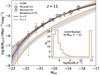 |
Fig. 4. Predicted UV luminosity function (Φ) at z = 11. Our standard ΛCDM model without PBHs (Sect. 2.2; solid orange curve) is compared with models including PBHs with λE = 0 (solid black) and λE = 1 (solid brown). The shaded regions denote the model uncertainties (16 and 84 percentiles at fixed MUV). The data from McLeod et al. (2024) and Donnan et al. (2024) at z = 11, and the fit from Bouwens et al. (2022a) to low-z data are also shown as a reference for our fiducial model. The inset shows the percentage of MUV = −21 galaxies that are hosted by halos of mass Mh for the λE = 1 case (brown line); the orange line is instead computed within the ΛCDM model without changing the normalization. Although the LF curves for both values of λE agree with data, they differ at the bright end of the LF. |
The inset in Fig. 4 shows the fraction of galaxies with MUV = −21 that are hosted by halos with mass Mh. In the standard ΛCDM model (and also in the λE = 0 case, not shown), the contribution comes from a single bin around 1011 M⊙. For λE = 1, instead, the distribution features a double-peak structure, with a high-mass (low-mass) peak produced by stellar (PBH-powered AGN) emission. As there is no significant difference in the rightmost part of the histograms, the bright-end LF enhancement is therefore mainly driven by galaxies in 108 − 9 M⊙ halos.
4. Discussion
PBHs have attracted considerable attention as possible dark matter candidates. These studies are limited in their predictions by our persisting ignorance of their typical mass, initial mass distribution, and abundance (Carr et al. 2021b). In Fig. 5 we report the currently available limits on monochromatic PBHs in the mass range relevant to the present study. The shaded regions correspond to combinations of parameters that differ from observations, and the stars represent our results. For simplicity, the constraints assume a monochromatic mass function, while results are reported as the peak of the posterior distribution we find. Lognormal mass functions usually have tighter limits due to the long tail of the distribution (Bellomo et al. 2018).
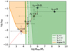 |
Fig. 5. PBH parameter exclusion plot in the fPBH − mPBH plane. We plot the constraint on the monochromatic PBH abundance from the CMB μ-distortion absence (Nakama et al. 2018, green lines) within different non-Gaussianity scenarios (fNL = 0, 10, ∞ represented by the solid, dashed, and dotted lines, respectively) and the one from the observed CMB angular power spectrum (Serpico et al. 2020, orange line). The shaded regions are excluded, and their colors denote the violated limit (same color scheme as for the lines). The stars and error bars give the results and uncertainty for different values of λE (Tab. 1). The dotted red line traces the expected trend for varying λE when only an AGN contribution is present. |
Between 102 M⊙ and 1010 M⊙, the two main constraints come from CMB observations. The first is from the undetected μ-distortion (Chluba et al. 2012; Nakama et al. 2018), and the second is obtained from the angular power spectrum (Serpico et al. 2020). The μ-distortion is a deviation in the CMB temperature distribution that may be caused by local heating due to PBHs when the age of the Universe was between 7 × 10⁶ s and 3 × 10⁹ s. In Fig. 5 the standard ΛCDM limit is reported as fNL = 0 (Gaussian fluctuations), while non-Gaussianity models are presented due to the loosening of constraints with higher fNL (we plot the cases fNL = 10, ∞). According to Planck Collaboration IX (2020), values of fNL > 10 are incompatible with observations. The CMB angular power spectrum limit is derived by computing the effect of accreting PBHs on the baryon angular distribution at the last scattering surface. Massive and abundant PBHs would indeed produce detectable patterns in the baryon density field.
The results we obtained in the case λE = 0 are compatible with those from Liu & Bromm (2022), who reported that fPBHmPBH ≳ 200 M⊙, mPBH ≳ 5 × 10⁸ M⊙ and σ = 0 (they considered only monochromatic PBHs) are required to explain JWST observations without assuming a high star formation efficiency. However, our λE = 0 solution leads to two problems: (i) At least a fraction of these massive black holes would probably accrete gas and emit with a detectable λE > 0, and (ii) the required abundance would be higher than the μ-distortion limits for their mass even for an extended mass function for PBHs. Allowing for PBH emission (λE > 0) ameliorates both issues as it automatically addresses the former and reconciles the results with the μ-distortion data constraints.
When considering high λE values, the mass function resulting from our study shifts toward lower-mass scales, evading the μ-distortion constraint. However, the angular power spectrum limit becomes dominant when MPBH ≲ 104 M⊙ (see Fig. 5), and values λE ≳ 10 provide consistent solutions to the problem.
The second solution found in the λE = 0.01 case violates the CMB angular power spectrum constraint even though much lower PBH masses are required than in the other cases. When comparing this solution with monochromatic limits, we must pay attention to the fact that the mass function is very wide: PBHs with mass ≈106 M⊙ are 2σ outliers, and their sole abundance is incompatible with μ-distortion limits, assuming that the constraint is not weakened by abundant low-mass PBHs.
Exploring diverse mass functions and considering even broader ones (e.g. García-Bellido et al. 2021) may provide useful insight on this topic and possibly find solutions that are compatible with CMB limits. Since results obtained by assuming extended mass functions are not reliably comparable with monochromatic constraints, a model-dependent analysis is required to solidly rule out the corresponding solutions. For example, Wang et al. (2025) reported looser constraints from the μ-distortion with a wide enough (σ ≳ 0.3) lognormal mass function when specific non-Gaussian primordial fluctuations models were assumed.
These considerations imply that the emission from PBHs acting as AGN is required for them to both explain the LF enhancement and comply with CMB observations. Moreover, our model entails that in 75% of the observed MUV = −21 sources at z ≈ 11 the emission should be dominated by an AGN (see the inset in Fig. 4), making it testable against spectroscopic observations. So far, spectroscopy on z ≳ 10 objects has revealed both AGN (e.g., UHZ1, Natarajan et al. 2024; GHZ2, Castellano et al. 2024) and star-forming galaxies (e.g., JADES-GS-z14-0, Carniani et al. 2024), but more data are required to provide a statistical sample to test our prediction.
We recall that we ignored the accretion of PBHs from their formation up to redshift z ≈ 11. To properly address this issue, further modeling of the PBH environment (Nayak & Jamil 2012; Jangra et al. 2024) is required. Naively, however, we note that if PBHs increase their mass by a factor 100 before z = 11 (as permitted by an efficient Bondi-Hoyle-Lyttleton accretion; see Jangra et al. 2024), they would explain JWST observation with λE being 100 times smaller than those found here (see Fig. B.1).
We also assumed that all PBH-powered AGN predicted by the model shine continuously and simultaneously, that is, we did not attempt to model the likely possibility that their duty cycle is < 1. In this case, a higher fPBH would be required to match the LF since a fraction of the PBHs would be quiescent. Unfortunately, the duty cycle would be degenerate with fPBH. Detailed numerical simulations could be useful to break this degeneracy.
5. Summary
We have investigated whether the inclusion of PBHs in the standard ΛCDM model can alleviate the problems raised by the observed excess of bright super-early (z > 10) galaxies. To do this, we computed the PBH contribution to the halo mass function (Sect. 2.1) and the galaxy LF (Sect. 2.3) for a lognormal initial PBH mass function (with a peak at MPBH and amplitude σ, Eq. 2), further assuming that they constitute a fraction fPBH of the dark matter and power an AGN with an Eddington ratio λE. Based on a Bayesian analysis (Sect. 2.5), we obtained the following results:
-
Although a small fraction (log fPBH ≈ −5.42) of massive (log MPBH/M⊙ ≈ 8.37 with σ ≈ 0.93), nonemitting (λE = 0) PBHs can explain the galaxy excess (Fig. B.1), this solution is in contrast with CMB μ-distortion constraints on monochromatic PBHs (Fig. 5) and must therefore be discarded.
-
If PBHs power an AGN that emits at super-Eddington luminosities (λE ≈ 10), the observed LF can be reproduced by a PBH population with a characteristic mass log MPBH/M⊙ ≈ 3.69, constituting a tiny (log fPBH ≈ −8.16) fraction of the cosmic dark matter content.
-
As λE and MPBH are degenerate, the LF remains unchanged when the degeneracy condition MPBHλE = 104.5 M⊙ is satisfied. A similar degeneracy exists between λE and fPBH (Eq. 10).
-
Although the LF can be reproduced by any set of (MPBH, λE) values satisfying the degeneracy condition, current CMB limits (Fig. 5) require that PBH-powered AGN emit at significant super-Eddington (λE ≳ 10) luminosities. This constraint can be overcome if PBHs grow by ≳10× their initial mass by the time of observation.
-
In the PBH scenario, about 75% of the observed galaxies with MUV = −21 at z = 11 should host a PBH-powered AGN and typically reside in low-mass halos, Mh = 108 − 9 M⊙ (Fig. 4). These predictions can be thoroughly tested with available and forthcoming JWST spectroscopic data.
Throughout the paper we assume a flat Universe with Planck Collaboration VI (2020) parameters Ωm = 0.30966, ΩΛ = 0.68885, Ωb = 0.04897, σ8 = 0.8102, and h = 0.6766, where Ωm, ΩΛ, Ωb are the matter, dark energy and baryon density ratios to the critical density, h is the Hubble constant in units of 100 km/s/Mpc and σ8 is the fluctuations’ rms amplitude parameter.
Since only PBHs have a Poisson noise term, in the initial perturbations isocurvature modes should be accounted for. The growth factor from Inman & Ali-Haïmoud (2019) refers to these fluctuations instead of the usual adiabatic ones.
We underline that the fit from Bouwens et al. (2022a) is performed directly on the LF, while we perform a fit on the MUV − Mh relation.
Acknowledgments
AF acknowledges support from the ERC Advanced Grant INTERSTELLAR H2020/740120. Partial support (AF) from the Carl Friedrich von Siemens-Forschungspreis der Alexander von Humboldt-Stiftung Research Award is kindly acknowledged. We gratefully acknowledge the computational resources of the Center for High Performance Computing (CHPC) at SNS. We acknowledge usage of WOLFRAM|ALPHA, the PYTHON programming language (Van Rossum & de Boer 1991; Van Rossum & Drake 2009), ASTROPY (Astropy Collaboration 2013), CORNER (Foreman-Mackey 2016), EMCEE (Foreman-Mackey et al. 2013), HMF (Murray et al. 2013), MATPLOTLIB (Hunter 2007), NUMPY (van der Walt et al. 2011), and SCIPY (Virtanen et al. 2020).
References
- Arrabal Haro, P., Dickinson, M., Finkelstein, S. L., et al. 2023, ApJ, 951, L22 [NASA ADS] [CrossRef] [Google Scholar]
- Astropy Collaboration (Robitaille, T. P., et al.) 2013, A&A, 558, A33 [NASA ADS] [CrossRef] [EDP Sciences] [Google Scholar]
- Atek, H., Shuntov, M., Furtak, L. J., et al. 2023, MNRAS, 519, 1201 [Google Scholar]
- Behroozi, P., Wechsler, R. H., Hearin, A. P., & Conroy, C. 2019, MNRAS, 488, 3143 [NASA ADS] [CrossRef] [Google Scholar]
- Behroozi, P., Conroy, C., Wechsler, R. H., et al. 2020, MNRAS, 499, 5702 [NASA ADS] [CrossRef] [Google Scholar]
- Bellomo, N., Bernal, J. L., Raccanelli, A., & Verde, L. 2018, JCAP, 2018, 004 [Google Scholar]
- Bhatt, M., Gallerani, S., Ferrara, A., et al. 2024, A&A, 686, A141 [NASA ADS] [CrossRef] [EDP Sciences] [Google Scholar]
- Biagetti, M., Franciolini, G., & Riotto, A. 2023, ApJ, 944, 113 [NASA ADS] [CrossRef] [Google Scholar]
- Bouwens, R. J., Oesch, P. A., Stefanon, M., et al. 2021, AJ, 162, 47 [NASA ADS] [CrossRef] [Google Scholar]
- Bouwens, R. J., Illingworth, G., Ellis, R. S., Oesch, P., & Stefanon, M. 2022a, ApJ, 940, 55 [NASA ADS] [CrossRef] [Google Scholar]
- Bouwens, R. J., Smit, R., Schouws, S., et al. 2022b, ApJ, 931, 160 [NASA ADS] [CrossRef] [Google Scholar]
- Bowler, R. A. A., Dunlop, J. S., McLure, R. J., et al. 2014, MNRAS, 440, 2810 [NASA ADS] [CrossRef] [Google Scholar]
- Bunker, A. J., Saxena, A., Cameron, A. J., et al. 2023, A&A, 677, A88 [NASA ADS] [CrossRef] [EDP Sciences] [Google Scholar]
- Carniani, S., Hainline, K., D’Eugenio, F., et al. 2024, Nature, 633, 318 [CrossRef] [Google Scholar]
- Carr, B., & Silk, J. 2018, MNRAS, 478, 3756 [NASA ADS] [CrossRef] [Google Scholar]
- Carr, B., Clesse, S., & García-Bellido, J. 2021a, MNRAS, 501, 1426 [Google Scholar]
- Carr, B., Kohri, K., Sendouda, Y., & Yokoyama, J. 2021b, Rep. Progr. Phys., 84, 116902 [Google Scholar]
- Casey, C. M., Akins, H. B., Shuntov, M., et al. 2024, ApJ, 965, 98 [NASA ADS] [CrossRef] [Google Scholar]
- Castellano, M., Fontana, A., Treu, T., et al. 2022, ApJ, 938, L15 [NASA ADS] [CrossRef] [Google Scholar]
- Castellano, M., Napolitano, L., Fontana, A., et al. 2024, ApJ, 972, 143 [Google Scholar]
- Chluba, J., Erickcek, A. L., & Ben-Dayan, I. 2012, ApJ, 758, 76 [Google Scholar]
- Ciesla, L., Elbaz, D., Ilbert, O., et al. 2024, A&A, 686, A128 [NASA ADS] [CrossRef] [EDP Sciences] [Google Scholar]
- Curtis-Lake, E., Carniani, S., Cameron, A., et al. 2023, Nat. Astron., 7, 622 [NASA ADS] [CrossRef] [Google Scholar]
- Dekel, A., Sarkar, K. C., Birnboim, Y., Mandelker, N., & Li, Z. 2023, MNRAS, 523, 3201 [NASA ADS] [CrossRef] [Google Scholar]
- Dolgov, A., & Silk, J. 1993, Phys. Rev. D, 47, 4244 [NASA ADS] [CrossRef] [Google Scholar]
- Donnan, C. T., McLeod, D. J., Dunlop, J. S., et al. 2023, MNRAS, 518, 6011 [Google Scholar]
- Donnan, C. T., McLure, R. J., Dunlop, J. S., et al. 2024, MNRAS, 533, 3222 [NASA ADS] [CrossRef] [Google Scholar]
- Feng, Y., Di Matteo, T., Croft, R., et al. 2015, ApJ, 808, L17 [Google Scholar]
- Feng, Y., Di-Matteo, T., Croft, R. A., et al. 2016, MNRAS, 455, 2778 [NASA ADS] [CrossRef] [Google Scholar]
- Ferrara, A., Pallottini, A., & Dayal, P. 2023, MNRAS, 522, 3986 [NASA ADS] [CrossRef] [Google Scholar]
- Ferrara, A., Pallottini, A., & Sommovigo, L. 2025, A&A, 694, A286 [NASA ADS] [CrossRef] [EDP Sciences] [Google Scholar]
- Finkelstein, S. L., Leung, G. C. K., Bagley, M. B., et al. 2024, ApJ, 969, L2 [NASA ADS] [CrossRef] [Google Scholar]
- Foreman-Mackey, D. 2016, J. Open Source Softw., 1, 24 [Google Scholar]
- Foreman-Mackey, D., Hogg, D. W., Lang, D., & Goodman, J. 2013, PASP, 125, 306 [Google Scholar]
- Fujimoto, S., Wang, B., Weaver, J. R., et al. 2024, ApJ, 977, 250 [NASA ADS] [CrossRef] [Google Scholar]
- García-Bellido, J., Carr, B., & Clesse, S. 2021, Universe, 8, 12 [Google Scholar]
- Gelli, V., Mason, C., & Hayward, C. C. 2024, ApJ, 975, 192 [NASA ADS] [CrossRef] [Google Scholar]
- Gouttenoire, Y., Trifinopoulos, S., Valogiannis, G., & Vanvlasselaer, M. 2024, Phys. Rev. D, 109, 123002 [Google Scholar]
- Green, A. M. 2016, Phys. Rev. D, 94, 063530 [NASA ADS] [CrossRef] [Google Scholar]
- Harvey, T., Conselice, C. J., Adams, N. J., et al. 2025, ApJ, 978, 89 [NASA ADS] [CrossRef] [Google Scholar]
- Hasinger, G. 2020, JCAP, 2020, 022 [CrossRef] [Google Scholar]
- Hsiao, T. Y.-Y., Abdurro’uf, Coe, D., et al. 2024, ApJ, 973, 8 [NASA ADS] [CrossRef] [Google Scholar]
- Hunter, J. D. 2007, Comput. Sci. Eng., 9, 90 [NASA ADS] [CrossRef] [Google Scholar]
- Inami, H., Algera, H. S. B., Schouws, S., et al. 2022, MNRAS, 515, 3126 [NASA ADS] [CrossRef] [Google Scholar]
- Inman, D., & Ali-Haïmoud, Y. 2019, Phys. Rev. D, 100, 083528 [NASA ADS] [CrossRef] [Google Scholar]
- Jangra, P., Gaggero, D., Kavanagh, B. J., & Diego, J. M. 2024, ArXiv e-prints [arXiv:2412.11921] [Google Scholar]
- Kannike, K., Marzola, L., Raidal, M., & Veermäe, H. 2017, JCAP, 2017, 020 [CrossRef] [Google Scholar]
- Klypin, A., Poulin, V., Prada, F., et al. 2021, MNRAS, 504, 769 [NASA ADS] [CrossRef] [Google Scholar]
- Labbé, I., van Dokkum, P., Nelson, E., et al. 2023, Nature, 616, 266 [CrossRef] [Google Scholar]
- Liu, B., & Bromm, V. 2022, ApJ, 937, L30 [NASA ADS] [CrossRef] [Google Scholar]
- Liu, B., Zhang, S., & Bromm, V. 2022, MNRAS, 514, 2376 [NASA ADS] [CrossRef] [Google Scholar]
- Manzoni, D., Ziparo, F., Gallerani, S., & Ferrara, A. 2024, MNRAS, 527, 4153 [Google Scholar]
- Mason, C. A., Trenti, M., & Treu, T. 2023, MNRAS, 521, 497 [NASA ADS] [CrossRef] [Google Scholar]
- McLeod, D. J., Donnan, C. T., McLure, R. J., et al. 2024, MNRAS, 527, 5004 [Google Scholar]
- Murray, S. G., Power, C., & Robotham, A. S. G. 2013, Astron. Comput., 3, 23 [CrossRef] [Google Scholar]
- Naidu, R. P., Oesch, P. A., van Dokkum, P., et al. 2022, ApJ, 940, L14 [NASA ADS] [CrossRef] [Google Scholar]
- Nakama, T., Carr, B., & Silk, J. 2018, Phys. Rev. D, 97, 043525 [NASA ADS] [CrossRef] [Google Scholar]
- Natarajan, P., Pacucci, F., Ricarte, A., et al. 2024, ApJ, 960, L1 [NASA ADS] [CrossRef] [Google Scholar]
- Nayak, B., & Jamil, M. 2012, Phys. Lett. B, 709, 118 [Google Scholar]
- Padmanabhan, H., & Loeb, A. 2023, ApJ, 953, L4 [NASA ADS] [CrossRef] [Google Scholar]
- Pallottini, A., & Ferrara, A. 2023, A&A, 677, L4 [NASA ADS] [CrossRef] [EDP Sciences] [Google Scholar]
- Pallottini, A., Ferrara, A., Gallerani, S., et al. 2024, A&A, submitted [arXiv:2408.00061] [Google Scholar]
- Planck Collaboration VI. 2020, A&A, 641, A6 [NASA ADS] [CrossRef] [EDP Sciences] [Google Scholar]
- Planck Collaboration IX. 2020, A&A, 641, A9 [Google Scholar]
- Press, W. H., & Schechter, P. 1974, ApJ, 187, 425 [Google Scholar]
- Robertson, B. E., Tacchella, S., Johnson, B. D., et al. 2023, Nat. Astron., 7, 611 [NASA ADS] [CrossRef] [Google Scholar]
- Robertson, B., Johnson, B. D., Tacchella, S., et al. 2024, ApJ, 970, 31 [NASA ADS] [CrossRef] [Google Scholar]
- Sabti, N., Muñoz, J. B., & Kamionkowski, M. 2024, Phys. Rev. Lett., 132, 061002 [Google Scholar]
- Serpico, P. D., Poulin, V., Inman, D., & Kohri, K. 2020, Phys. Rev. Res., 2, 023204 [NASA ADS] [CrossRef] [Google Scholar]
- Shen, X., Hopkins, P. F., Faucher-Giguère, C.-A., et al. 2020, MNRAS, 495, 3252 [Google Scholar]
- Shen, X., Vogelsberger, M., Boylan-Kolchin, M., Tacchella, S., & Naidu, R. P. 2024, MNRAS, 533, 3923 [Google Scholar]
- Sheth, R. K., & Tormen, G. 2002, MNRAS, 329, 61 [Google Scholar]
- Sun, G., Faucher-Giguère, C.-A., Hayward, C. C., et al. 2023, ApJ, 955, L35 [CrossRef] [Google Scholar]
- Sun, G., Muñoz, J. B., Mirocha, J., & Faucher-Giguère, C. A. 2024, JCAP, submitted [arXiv:2410.21409] [Google Scholar]
- van der Walt, S., Colbert, S. C., & Varoquaux, G. 2011, Comput. Sci. Eng., 13, 22 [Google Scholar]
- Van Rossum, G., & de Boer, J. 1991, CWI Quarterly, 4, 283 [Google Scholar]
- Van Rossum, G., & Drake, F. L. 2009, Python 3 Reference Manual (Scotts Valley, CA: CreateSpace) [Google Scholar]
- Vijayan, A. P., Lovell, C. C., Wilkins, S. M., et al. 2021, MNRAS, 501, 3289 [NASA ADS] [Google Scholar]
- Virtanen, P., Gommers, R., Oliphant, T. E., et al. 2020, Nat. Meth., 17, 261 [Google Scholar]
- Vogelsberger, M., Nelson, D., Pillepich, A., et al. 2020, MNRAS, 492, 5167 [NASA ADS] [CrossRef] [Google Scholar]
- Wang, B., Fujimoto, S., Labbé, I., et al. 2023, ApJ, 957, L34 [NASA ADS] [CrossRef] [Google Scholar]
- Wang, Z. H., Huang, H. L., & Piao, Y. S. 2025, ArXiv e-prints [arXiv:2501.08542] [Google Scholar]
- Wilkins, S. M., Feng, Y., Di Matteo, T., et al. 2017, MNRAS, 469, 2517 [NASA ADS] [CrossRef] [Google Scholar]
- Zavala, J. A., Castellano, M., Akins, H. B., et al. 2025, Nat. Astron., 9, 155 [Google Scholar]
Appendix A: PBH contribution to the power spectrum with lognormal IMF
We took a lognormal as the fiducial model for the PBH mass function
 (A.1)
(A.1)
where n0 is the number density scale; n0 can be connected to fPBH from
 (A.2a)
which implies
 (A.2b)
The corresponding fraction of dark matter mass in PBH of mass M is:
 (A.3)
(A.3)
Inverting the relation for kcrit in eq. 1 combined with eq. 1c, it is possible to define
 (A.4)
(A.4)
as the mass associated with a given critical wavenumber. The power spectrum contribution can then be computed as follows:
 (A.5)
(A.5)
Although it is not explicit from eq. A.5, in the limit σ → 0 we effectively recover the term in eq. 1. This expression is also convenient to avoid numerical problems with the derivation of the power spectrum around the scale of kcrit.
Appendix B: Posterior corner plot
For a better visualization of MCMC results, we plot in Fig. B.1 the posterior distribution described in Sec. 3.
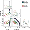 |
Fig. B.1. Corner plot of the posterior for the PBH models (Sec. 2). The parameters describing the mass function of the PBHs (eq. 2) are obtained via the MCMC using constraints at z = 11 and assuming PBHs are distributed independently of halo mass. Each color corresponds to a value for λE, as reported in the legend. An interesting feature to note is that, as long as λE > 0.01, changing λE shifts the posterior distribution, as indicated in eq. 10. Tabulated results are reported in Tab. 1. |
Appendix C: Alternative parametrization of results
In the case of a monochromatic mass function for PBHs, the power spectrum enhancement is completely degenerate in fPBH and mPBH. For this reason, in Fig. C.1 and Tab. C.1 we report the results from Sec. 3 with an alternative parametrization (product and ratio of fPBH and MPBH) that may be useful to compare with other works.
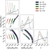 |
Fig. C.1. Alternative corner plot of the posterior for the PBH models (Sec. 2). Parameters resulting from the MCMC procedure (see Fig. B.1 and Tab. 1) have been recombined in the form of log(fPBHMPBH/M⊙) and log(MPBH/fPBH/M⊙). Each color corresponds to a value for λE, as reported in the legend. Tabulated results are reported in Tab. C.1. |
Tabulated MCMC results for the alternative parametrization.
All Tables
All Figures
|
Fig. 1. Overview of the modifications to the HMF due to the PBH contribution to the power spectrum. The Sheth & Tormen (2002) HMF (n) at z = 11 is plotted as a function of halo mass (Mh) for a pure ΛCDM cosmology and for PBHs with lognormal mass functions, constituting a fraction fPBH = 10−5 of the total dark matter density; each color corresponds to a different PBH mass MPBH = 109 M⊙, 1011 M⊙, whereas continuous (dashed) lines represent monochromatic (lognormal with σ = 0.5) mass functions. For reference, we show the corresponding power spectra at z = 0 (PCDM, Eq. 1) as a function of the wavenumber (k) as an inset. |
| In the text | |
|
Fig. 2. Ultraviolet luminosity function of galaxies (Φ) at different redshifts compared to data (Bouwens et al. 2021, 2022a). The LF from our model (solid line, Eq. 4) was fit to the points at the reported redshifts (parameters in Eq. 5). |
| In the text | |
|
Fig. 3. Ultraviolet magnitude (MUV) as a function of Mh at z = 9 within different models. The relation in this work is obtained via a fit of the LF (see Eq. 4 for the functional form and Eq. 5 for the parameters). For comparison, we report MUV(Mh) from the semi-analytical model of Ferrara et al. (2023, in the dust-attenuated, DA, and attenuation-free, AF, cases), from the abundance-matching based procedure of Behroozi et al. (2019) and results from the BlueTides hydrodynamical simulations (Wilkins et al. 2017). |
| In the text | |
|
Fig. 4. Predicted UV luminosity function (Φ) at z = 11. Our standard ΛCDM model without PBHs (Sect. 2.2; solid orange curve) is compared with models including PBHs with λE = 0 (solid black) and λE = 1 (solid brown). The shaded regions denote the model uncertainties (16 and 84 percentiles at fixed MUV). The data from McLeod et al. (2024) and Donnan et al. (2024) at z = 11, and the fit from Bouwens et al. (2022a) to low-z data are also shown as a reference for our fiducial model. The inset shows the percentage of MUV = −21 galaxies that are hosted by halos of mass Mh for the λE = 1 case (brown line); the orange line is instead computed within the ΛCDM model without changing the normalization. Although the LF curves for both values of λE agree with data, they differ at the bright end of the LF. |
| In the text | |
|
Fig. 5. PBH parameter exclusion plot in the fPBH − mPBH plane. We plot the constraint on the monochromatic PBH abundance from the CMB μ-distortion absence (Nakama et al. 2018, green lines) within different non-Gaussianity scenarios (fNL = 0, 10, ∞ represented by the solid, dashed, and dotted lines, respectively) and the one from the observed CMB angular power spectrum (Serpico et al. 2020, orange line). The shaded regions are excluded, and their colors denote the violated limit (same color scheme as for the lines). The stars and error bars give the results and uncertainty for different values of λE (Tab. 1). The dotted red line traces the expected trend for varying λE when only an AGN contribution is present. |
| In the text | |
|
Fig. B.1. Corner plot of the posterior for the PBH models (Sec. 2). The parameters describing the mass function of the PBHs (eq. 2) are obtained via the MCMC using constraints at z = 11 and assuming PBHs are distributed independently of halo mass. Each color corresponds to a value for λE, as reported in the legend. An interesting feature to note is that, as long as λE > 0.01, changing λE shifts the posterior distribution, as indicated in eq. 10. Tabulated results are reported in Tab. 1. |
| In the text | |
|
Fig. C.1. Alternative corner plot of the posterior for the PBH models (Sec. 2). Parameters resulting from the MCMC procedure (see Fig. B.1 and Tab. 1) have been recombined in the form of log(fPBHMPBH/M⊙) and log(MPBH/fPBH/M⊙). Each color corresponds to a value for λE, as reported in the legend. Tabulated results are reported in Tab. C.1. |
| In the text | |
Current usage metrics show cumulative count of Article Views (full-text article views including HTML views, PDF and ePub downloads, according to the available data) and Abstracts Views on Vision4Press platform.
Data correspond to usage on the plateform after 2015. The current usage metrics is available 48-96 hours after online publication and is updated daily on week days.
Initial download of the metrics may take a while.