| Issue |
A&A
Volume 685, May 2024
|
|
|---|---|---|
| Article Number | A31 | |
| Number of page(s) | 14 | |
| Section | Astrophysical processes | |
| DOI | https://doi.org/10.1051/0004-6361/202348903 | |
| Published online | 30 April 2024 | |
Heavy black hole seed formation in high-z atomic cooling halos
1
Centre for Astrophysics and Space Science Maynooth, Department of Theoretical Physics, Maynooth University, Maynooth, Ireland
e-mail: lewis.prole@mu.ie
2
Universität Heidelberg, Zentrum für Astronomie, Institut für Theoretische Astrophysik, Albert-Ueberle-Straße 2, 69120 Heidelberg, Germany
3
Universität Heidelberg, Interdisziplinäres Zentrum für Wissenschaftliches Rechnen, Im Neuenheimer Feld 205, 69120 Heidelberg, Germany
4
Cardiff University School of Physics and Astronomy, Cardiff, UK
Received:
11
December
2023
Accepted:
15
February
2024
Context. Halos with masses in excess of the atomic limit are believed to be ideal environments in which to form heavy black hole seeds with masses above 103 M⊙. In cases where the H2 fraction is suppressed, this is expected to lead to reduced fragmentation of the gas and the generation of a top-heavy initial mass function. In extreme cases this can result in the formation of massive black hole seeds. Resolving the initial fragmentation scale and the resulting protostellar masses has, until now, not been robustly tested.
Aims. We run zoom-in simulations of atomically cooled halos in which the formation of H2 is suppressed to assess whether they can truly resist fragmentation at high densities and tilt the initial mass function towards a more top-heavy form and the formation of massive black hole seeds.
Methods. Cosmological simulations were performed with the moving mesh code AREPO, using a primordial chemistry network until z ∼ 11. Three haloes with masses in excess of the atomic cooling mass were then selected for detailed examination via zoom-ins. A series of zoom-in simulations, with varying levels of maximum spatial resolution, captured the resulting fragmentation and formation of metal-free stars using the sink particle technique. The highest resolution simulations resolved densities up to 10−6 g cm−3 (1018 cm−3) and captured a further 100 yr of fragmentation behaviour at the centre of the halo. Lower resolution simulations were then used to model the future accretion behaviour of the sinks over longer timescales.
Results. Our simulations show intense fragmentation in the central region of the halos, leading to a large number of near-solar mass protostars. Even in the presence of a super-critical Lyman-Werner radiation field (JLW > 105J21), H2 continues to form within the inner ∼2000 au of the halo. Despite the increased fragmentation, the halos produce a protostellar mass spectrum that peaks at higher masses relative to standard Population III star-forming halos. The most massive protostars have accretion rates of 10−3–10−1 M⊙ yr−1 after the first 100 years of evolution, while the total mass of the central region grows at 1 M⊙ yr−1. Lower resolution zoom-ins show that the total mass of the system continues to accrete at ∼1 M⊙ yr−1 for at least 104 yr, although how this mass is distributed amongst the rapidly growing number of protostars is unclear. However, assuming that a fraction of stars can continue to accrete rapidly, the formation of a sub-population of stars with masses in excess of 103 M⊙ is likely in these halos. In the most optimistic case, we predict the formation of heavy black hole seeds with masses in excess of 104 M⊙, assuming an accretion behaviour in line with expectations from super-competitive accretion and/or frequent mergers with secondary protostars.
Key words: stars: black holes / stars: Population III / quasars: supermassive black holes / dark ages / reionization / first stars
© The Authors 2024
 Open Access article, published by EDP Sciences, under the terms of the Creative Commons Attribution License (https://creativecommons.org/licenses/by/4.0), which permits unrestricted use, distribution, and reproduction in any medium, provided the original work is properly cited.
This article is published in open access under the Subscribe to Open model. Subscribe to A&A to support open access publication.
1. Introduction
Quasi-stellar radio sources (quasars) are thought to be powered by supermassive black holes (SMBHs) which populate the centres of most, if not all, massive galaxies. Quasars have been detected out to redshifts of z > 7 with black hole (BH) masses believed to be in excess of 109 M⊙ (e.g., Mortlock et al. 2011; Matsuoka et al. 2019; Fan et al. 2023), implying that the seeds for these SMBHs formed in the early Universe. The existence of SMBHs with masses in excess of 109 M⊙ within the first billion years of the Universe poses a challenge to our understanding of both BH formation and BH accretion. Two mainstream pathways have emerged over the last four decades to explain how such massive objects appear so early in cosmic history; SMBHs may originate from so-called light seeds with masses less than 103 M⊙, or from heavy BH seeds with masses significantly in excess of 103 M⊙.
Light seeds are typically thought to form from the remnants of the first stars - Population III (Pop III) stars, which form in dark matter minihalos collapsing at a mass threshold of ∼106 M⊙. Initial ab initio modelling of Pop III star formation predicted an extremely top-heavy IMF for the first stars (e.g., Bromm et al. 1999, 2001; Abel et al. 2002) with characteristic masses of order 1000 M⊙. However, more recent studies throughout the last decade have found that Pop III stellar masses are lower than initially suggested (e.g., Stacy et al. 2010; Clark et al. 2011; Hirano et al. 2014; Susa 2019; Latif et al. 2022a; Prole et al. 2023; for a recent review see Klessen & Glover 2023) with characteristic masses of a few tens of M⊙. Depending on the exact onset of BH formation these light seeds would need to maintain accretion at the Eddington rate for several hundred million years in order to bridge the approximately seven orders of magnitude in mass required to reach the upper limits of the SMBH threshold. Alternatively, periods of super-Eddington accretion may offer a solution. In this case the light seed BH can grow at supra-exponential rates (Alexander & Natarajan 2014) which only need to last for brief periods of time (Lupi et al. 2016; Inayoshi et al. 2016). However, in both Eddington-limited and super-Eddington cases, radiative feedback from the accretion of matter onto BHs heats the surrounding gas and lowers the accretion rate (Johnson & Bromm 2007; Milosavljević et al. 2009; Alvarez et al. 2009; Smith et al. 2018) – making maintaining either Eddington accretion and/or super-Eddington accretion unlikely over sustained periods (Regan et al. 2019; Su et al. 2023; Massonneau et al. 2023). Finally, both Eddington and super-Eddington-limited growth require that the light seed sit at the centre of a powerful gas inflow and that the embryonic BH can readily accrete the surrounding dense gas. However, dynamical studies of BHs have shown that this is also a challenge, with light seeds tending to walk random trajectories around the host halo centres (Beckmann et al. 2019; Pfister et al. 2019). As a result of these obstacles to light seed growth, the possibility of much heavier BH seeds has also been studied, beginning with Rees (1978).
Forming heavy seeds has hinged on two separate but not necessarily distinct pathways. On the one hand dynamical processes have been invoked to explain heavy BH seed formation; runaway collisions in dense young star clusters could produce massive black holes (MBHs) of ∼103 M⊙ (e.g., Portegies Zwart et al. 2004; Glebbeek et al. 2009; Katz et al. 2015; Reinoso et al. 2023) that are candidates for the ultraluminous X-ray sources observed in young star-forming regions (Ptak & Colbert 2004). These MBHs may grow into SMBHs through binary mergers and/or gas accretion (Micic et al. 2007). BH mergers within a dense BH cluster may achieve the same outcome (Stone et al. 2017; Schleicher et al. 2022) through either collisions and/or gas accretion, although the growth prospects are far from certain (Arca Sedda et al. 2023). Additionally, SMBHs may form directly via galaxy mergers (Mayer et al. 2010; Mayer & Bonoli 2018).
On the other hand, conditions may exist in the early Universe conducive to the formation of truly massive stars with final masses well in excess of 103 M⊙ (Regan et al. 2020, 2023; Latif et al. 2022b) and possibly up as high as a few times 105 M⊙ (Woods et al. 2017). The formation of these massive primordial Pop III stars requires high inflow rates onto the stellar surface (Hosokawa & Omukai 2009; Hosokawa et al. 2012), but repeated numerical experiments have shown the stars to be stable for at least 2 Myr until their inevitable direct collapse into a MBH (e.g., Haemmerlé et al. 2018; Woods et al. 2020). Finally, it may also be that the processes that lead to a dense stellar cluster or a massive Pop III star form part of a continuum with a massive star-forming at the very centre of a dense stellar cluster, where collisions drive the formation of a very massive star (Boekholt et al. 2018; Chon & Omukai 2020; Schleicher et al. 2023).
Halos can reach masses surpassing the canonical minihalo mass of 106 M⊙ without experiencing star formation (in a ΛCDM cosmology) at the rare intersection of strong accretion flows in low shear environments (Tenneti et al. 2018; Huang et al. 2018). These haloes may then be capable of forming heavy BH seeds (Smidt et al. 2018; Wise et al. 2019; Zhu et al. 2022; Latif et al. 2022b). Here, highly supersonic turbulence, due to the powerful accretion streams, prevents collapse and subsequent star formation in the halo until it reaches a mass threshold of a few 107 M⊙, resulting in higher accretion rates on the central objects. Alternatively, additional physical factors have been shown to boost halo masses prior to star formation, most prominently dark matter-baryon streaming motions and Lyman-Werner (LW) radiation backgrounds, which lead to the formation of so-called atomically cooled halos. This paper focuses on the latter (super-critical LW flux), and aims to test whether atomically cooled halos can lead to the formation of a heavy seed Pop III star using state-of-the-art, high resolution, hydrodynamic simulations.
Pristine atomic cooling halos have long been suggested as the ideal environment in which to seed MBHs (Loeb & Rasio 1994; Spaans & Silk 2006; Prieto et al. 2013). If the H2 abundance inside the massive halo can be suppressed, the gas must cool predominatly through atomic hydrogen line emission and H− free-bound emission. The thermal pathway then taken by the gas inside an atomic cooling halo in the absence of effective H2 cooling deviates significantly from the standard Pop III star formation scenario (e.g., Omukai 2000; Klessen & Glover 2023).
Pop III star formation in minihalos is facilitated by molecular hydrogen. The DM halo potential well pulls in the gas and shock heats it up to ∼1000 K, At these temperatures, the H2 abundance increases to ∼10−4 (e.g., Tegmark et al. 1997; Greif et al. 2008) where rotational transitions can occur via electrical quadrupole radiation, which allows the gas to cool down to minimum temperatures of ∼200 K (e.g., Abel et al. 1997; Bromm et al. 1999; Glover & Abel 2008) and collapse, decoupling from the DM halo.
One potential way in which H2 abundances can be reduced is via a nearby source of LW radiation. These far-ultraviolet (FUV) photons in the Lyman and Werner bands of H2 (11.2–13.6 eV) can dissociate H2 via the two-step Solomon process (Field et al. 1966; Stecher & Williams 1967). Additionally, photons of above 0.76 eV can photodissociate H−, disrupting the primary H2 formation channel (e.g., Chuzhoy et al. 2007). Before the Strömgren spheres of Pop III stars overlap, the UV background below the ionisation threshold is able to penetrate large clouds and suppress their H2 abundance (Haiman et al. 1997). This photodissociation of H2 suppresses further star formation inside small halos and delays reionisation until larger halos form (Haiman et al. 2000). While other physical mechanism can have a similar effect, we are focused here in studying the gas collapse inside atomically cooling halos, which are both pristine and have had their H2 cooling efficiency suppressed.
In halos with virial temperatures below Tvir ∼ 8000 K, star formation is suppressed entirely if LW radiation reduces the H2 abundance below the level at which gas can cool within a Hubble time. For example, an intense burst of LW radiation from a neighbouring star-bursting protogalaxy just before the gas cloud undergoes gravitational collapse is proposed to prevent the cloud from collapsing or forming stars (Regan et al. 2017). However, the halo will continue to grow through hierarchical mergers (e.g., Chon et al. 2016; Dong et al. 2022). Once the virial temperature reaches ∼8000 K, it becomes possible for the gas to cool via Lyman-α emission. The required virial temperature is related to the virial mass through the relation (Fernandez et al. 2014)
giving a virial mass of ∼3 × 10⁷ M⊙ at z = 12 for a virial temperature of 8000 K. If a halo can grow to this mass it will become hot enough to cool via atomic line emission and begin to collapse (Oh & Haiman 2002; Bromm & Loeb 2003; Bromm & Yoshida 2011). In this scenario, the collapse occurs almost isothermally, and fragmentation of the gas is thought to be suppressed throughout.
The maximum density that can be reached in simulations of this process is related to the resolution of the simulation. To avoid artificial fragmentation, it is necessary to resolve the Jeans length, which progressively shrinks as the gas collapses to higher densities (Truelove et al. 1997). Therefore, the better the resolution of the simulation, the higher the density that it can reach. We know from simulations of the standard Pop III star formation scenario that the formation of the primordial protostar occurs at densities of 10−6–10−4 g cm−3 where the gas becomes adiabatic (Omukai 2000; Machida & Nakamura 2015). The Jeans length at this stage is 0.01-0.1 au, and so the required resolution is roughly a factor of ten smaller than this. Despite this, the resolution of most atomically cooled halo simulations is relatively poor in comparison, with most studies not resolving their gas past densities of 10−17 g cm−3 (e.g. Shang et al. 2010; Sugimura et al. 2014; Regan et al. 2014, 2017; Hartwig et al. 2015; Agarwal & Khochfar 2015; Glover 2015; Agarwal et al. 2016; Dunn et al. 2018). This resolution is sufficient to determine whether or not H2 cooling is important during the initial collapse of the gas, but does not allow one to draw conclusions about the later stages of the collapse. Some studies find evidence for small-scale fragmentation, even in the absence of effective H2 cooling (e.g. Becerra et al. 2015, 2018a; Chon et al. 2018; Suazo et al. 2019; Latif et al. 2020; Patrick et al. 2023). The number of fragments formed is generally much smaller than the number found in recent simulations of the standard Pop III star formation scenario. However, this may be a consequence of the limited peak density: in most of these studies, the gas density never exceeds ρ ∼ 10−10 g cm−3, four orders of magnitude smaller than the point at which we expect the collapse to become adiabatic (Becerra et al. 2018b). Studies that resolve atomically cooled halos up to near protostellar densities have only simulated the first few years after the formation of the first protostar, hence the sustained fragmentation and accretion behaviour is unknown (Inayoshi et al. 2014; Becerra et al. 2015).
This study aims to provide the most accurate picture of atomically cooled halo collapse at high densities to date, answering whether atomic cooling halos do experience reduced fragmentation and higher stellar or BH seed masses compared to the Pop III minihalo scenario, or whether the fragmentation at high densities produces protostellar masses similar to what we have seen in simulations of Pop III star-forming minihalos. To that end, we simulate the collapse of atomically cooled halos from cosmological initial conditions with zoom-in simulations running up to the lower limit of protostellar formation at 10−6 g cm−3 and capturing a further ∼100 yr of disc fragmentation. We directly compare our results to a recent study, Prole et al. (2023; hereafter LP23) which examined H2 cooling minihalos with the same simulation code, chemical set-up and maximum resolution as the simulations presented in this work.
The format of this paper is as follows: in Sect. 2 we outline the numerical technique used including the simulation code and chemical network. In Sect. 3 we discuss the collapse of the gas up to point immediately prior to sink formation, while in Sect. 4 we discuss the fragmentation of the gas after the insertion of sink particles. In Sect. 5 we analyse the growth of the stellar system and compare, via a convergence study, the evolution of the star particles into main sequence stars and discuss their eventual evolution into (massive) BHs. In Sect. 6 we discuss some caveats before concluding in Sect. 7.
2. Numerical method
2.1. AREPO
The simulations presented here were performed with the moving mesh code AREPO (Springel 2010) with a primordial chemistry set-up described in Sect. 2.2. AREPO combines the advantages of adaptive mesh refinement (AMR: Berger & Colella 1989) and smoothed particle hydrodynamics (SPH: Monaghan 1992) with a mesh made up of a moving, unstructured, Voronoi tessellation of discrete points. AREPO solves hyperbolic conservation laws of ideal hydrodynamics with a finite volume approach, based on a second-order unsplit Godunov scheme with an exact Riemann solver. Automatic and continuous refinement overcome the challenge of structure growth associated with AMR (e.g., Heitmann et al. 2008).
2.2. Chemistry
Collapse of primordial gas is closely linked to the chemistry involved (e.g., Glover et al. 2006; Yoshida et al. 2007; Glover & Abel 2008; Turk et al. 2011). We therefore use a fully time-dependent chemical network to model the gas. We use the treatment of primordial chemistry and cooling originally described in Clark et al. (2011), but with updated values for some of the rate coefficients, as summarised in Schauer et al. (2019). The network has 45 chemical reactions to model primordial gas made up of 12 species: H, H+, H−, H , H2, He, He+, He++, D, D+, HD and free electrons. Optically thin H2 cooling is modelled as described in Glover & Abel (2008): we first calculate the rates in the low density (n → 0) and LTE limits, and the smoothly interpolate between them as a function of n/ncr, where ncr is the H2 critical number density above which collisions are so frequent that they keep the populations close to their LTE values. To compute the H2 cooling rate in the low density limit, we account for the collisions with H, H2, He, H+ and electrons. To calculate the H2 cooling rate in the optically thick limit, we use an approach based on the Sobolev approximation (Yoshida et al. 2006; Clark et al. 2011). Prior to the simulation, we compute a grid of optically thick H2 cooling rates as a function of the gas temperature and H2 column density. During the simulation, if the gas is dense enough for the H2 cooling to potentially be in the optically thick regime (ρ > 2 × 10⁻¹⁶ g cm−3), we interpolate the H2 cooling rate from this table, using the local gas temperature and an estimate of the effective H2 column density computed using the Sobolev approximation. In addition to H2 cooling, we also account for several other heating and cooling processes: cooling from atomic hydrogen and helium, collisionally induced H2 emission, HD cooling, ionisation and recombination, heating and cooling from changes in the chemical make-up of the gas and from shocks, compression and expansion of the gas, three-body H2 formation and heating from accretion luminosity. For reasons of computational efficiency, the network switches off tracking of deuterium chemistry1 at densities above 10−16 g cm−3, instead assuming that the ratio of HD to H2 at these densities is given by the cosmological D to H ratio of 2.6 × 10⁻⁵. We note that although our treatment of H2 cooling accounts for the opacity of the gas at high densities, our treatment of the effects of other cooling processes, such as H− free-bound emission, does not currently account for the continuum opacity of the gas. At densities below ∼10−8 g cm−3, this makes little difference to the thermal evolution of the gas, but it means that we tend to overestimate the cooling rate at densities above this value. The adiabatic index of the gas is computed as a function of chemical composition and temperature with the AREPO HLLD Riemann solver.
2.3. Simulation setup
As discussed in the Introduction the goal of this study is to investigate the formation of primordial Pop III stars at the centre of a metal-free atomically cooling halo. Such halos have previously been investigated as ideal sites for heavy seed formation (Haiman et al. 1996; Regan & Haehnelt 2009; Latif et al. 2013d, 2015, 2020; Latif & Volonteri 2015; Wise et al. 2019). To generate the appropriate initial conditions we generated cosmological initial conditions using MUSIC (Hahn & Abel 2011). An initial cosmological simulation was performed within a co-moving box of side length 1 h−1 Mpc using a ΛCDM cosmology with parameters h = 0.6774, Ω0 = 0.3089, Ωb = 0.04864, ΩΛ = 0.6911, n = 0.96 and σ8 = 0.8159 (Planck Collaboration VI 2020). The simulations were initialised at z = 127 with an initial dark matter distribution using the transfer functions of Eisenstein & Hu (1998). The gas distribution was set within AREPO to initially follow the dark matter (i.e., GENERATE_GAS_IN_ICS = 1). We model the dark matter with 5123 particles and the gas was modelled with 5123 grid cells (prior to refinement). During the simulation, an additional Jeans refinement criterion was applied such that the Jeans length of the gas is always resolved with at least 4 grid cells. Hence, the gas is able to dynamically refine during the simulation allowing maximum resolution where required.
During this initial phase, we disabled the molecular chemistry functionality and hence utilised a simpler 6 species model such that H2 and HD abundances remained at their initial value. This eliminated the need for a LW background radiation field at this initial stage of the calculation since the goal of this study is to investigate the idealised case of Pop III formation inside of a pristine, atomically cooling halo at a virial temperature of approximately 8000 K. We note that applying a super-critical LW field has the same result on the H2 abundance. As the dominant HD formation pathway relies on the H2 abundance (Nakamura & Umemura 2002), a super-critical LW field also suppresses the HD abundance.
At z ∼ 13.3 the first atomic halo begins to collapse within our box. Two more, physically distinct halos collapse at z = 11.5. These first three halos to begin atomically cooling and collapsing were then extracted. The selection criteria was simple; while H2 rich halos begin cooling down from 1000 K from ∼10−23 g cm−3, reaching 200 K by ∼10−22 g cm−3, we have disabled H2 formation, hence the only way for the gas to collapse to these densities is via atomic cooling. A density threshold for selecting a collapsing halo was therefore chosen as slightly higher than this density at 10−21 g cm−3. Only halos containing gas cells with a density exceeding this threshold were selected for extraction and resimulation. The central coordinate of the halos was found using a friends of friends (FoF) algorithm and a new box length of 2 kpc (physical units) was cut around it. Using the new box cut from the parent box, the simulations were restarted as zoom-in simulations. The units were converted into physical units for the remainder of the zoom-in calculation and the simulation essentially run as an isolated galaxy simulation with periodic boundary conditions. Table 1 shows the virial mass, radius and temperature of each halo as calculated by the FoF algorithm as well as the redshift when it was extracted, while Fig. 1 shows the temperature-density profiles at that stage and Fig. 2 shows the radial profiles of the enclosed mass for both the gas and the DM.
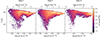 |
Fig. 1. 2D histograms of the temperature – density profiles for the halos at the point at which they were extracted from the initial cosmological simulation, weighted by total gas mass within each 2D bin. The halos have begun to gravitationally collapse via atomic cooling as seen from the close to isothermal temperature profile. They differ from the regular H2 minihalo case by the absence of a sharp drop in temperature to ∼200 K beginning at ∼10−23 g cm−3. |
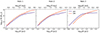 |
Fig. 2. Radial profiles of enclosed gas and DM mass for the three atomic halos at the point where they were extracted from the initial cosmological simulation. The baryonic component becomes comparable to the DM within the central ∼100 pc where it begins to decouple from the DM. In Halo 3, the baryonic component is dominant over DM on these scales. |
Halo virial masses, radii, and temperatures along with redshifts at the point where they were extracted from the initial cosmological simulation.
For the zoom-in simulations, the full chemistry model (12 species) is again enabled to get an accurate picture of H2 formation at very high densities inside the core of the collapsing halo. We invoke a blackbody radiation spectrum at temperature 105 K to model the expected emission from Pop III stars, with a super-critical LW radiation intensity of JLW = 105J21 (where J21 is in units of 10−21 erg s−1 cm−2 Hz−1 sr−1) to suppress H2 formation. We model the effects of H2 self-shielding using the TreeCol algorithm (Clark et al. 2012). We note that H− photodetachment via IR photons is also included.
We turn-on the 12 species model to examine the impact of H2 production which is inevitable at the highest densities. In our highest resolution simulations, we evolve the collapse up to a density of 10−6 g cm−3 before inserting sink particles (see Sect. 2.5) and capturing a further ∼100 yr of disc fragmentation and accretion behaviour, while in the lowest resolution simulation we capture ∼104 yr of accretion. See Table 2 for a list of simulation realisations and resolutions employed. The structure of Halo 3 at the end of the high resolution simulation is visualised in Fig. 3, which shows the density field along with H2 fraction and temperatures at various zoom-in scales.
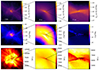 |
Fig. 3. Projection images of the zoom-in simulation box, showing density, H2 fraction and temperature for Halo 3 at the end of the simulation. From left to right, the zoom-in plots show at radius of 1 kpc, 10 pc and 0.1 pc, respectively. |
Simulation parameters.
2.4. Low resolution re-simulations
As our high resolution simulations are only able to evolve for approximately one hundred years after the formation of the first protostar due to their extreme computational cost, it is not possible to directly determine the zero age main sequence mass of the stars formed in the system. We therefore re-run the simulation of Halo 3 with lower resolution to make an estimate of protostellar growth on longer timescales. The resolution study presented in Prole et al. (2022a) found that the total mass accreted across all sink particles is well estimated by low resolution simulations, with less fragmentation yielding higher mass protostars. Our lower resolution simulations can therefore estimate the total mass in sink particles long after the high resolution simulations end. Since the three atomically cooled halos examined here have a similar total sink particle mass evolution (see Sect. 4), we only re-ran lower resolution simulations of Halo 3, which should nonetheless be a good proxy for all three halos.
We chose to re-run the simulation with threshold sink particle creation densities of 10−13 and 10−10 g cm−3, changing the minimum cell volume and gravitational softening lengths appropriately (see Sect. 2.5 for details). The three different density threshold simulations will be referred to as high, medium and low resolution from here on, although we emphasise that even the low resolution simulations have an extremely high spatial resolution of ∼300 au.
2.5. Sink particles
The simulation mesh must be refined during a gravitational collapse to ensure the local Jeans length is resolved. Once the mesh refines down to its minimum cell volume, sink particles must be introduced to represent the dense gas, preventing artificial instability in cells larger than their Jeans length. Our sink particle implementation was introduced in Wollenberg et al. (2020) and Tress et al. (2020). A cell is converted into a sink particle if it satisfies three criteria:
-
The cell reaches a threshold density.
-
It is sufficiently far away from pre-existing sink particles so that their accretion radii do not overlap.
-
The gas occupying the region inside the sink is gravitationally bound and collapsing.
Likewise, for the sink particle to accrete mass from surrounding cells, the cell must meet two criteria:
-
The cell lies within the accretion radius.
-
It is gravitationally bound to the sink particle.
A sink particle can accrete up to 90% of a cell’s mass, above which the cell is removed and the total cell mass is transferred to the sink.
Increasing the threshold density for sink particle creation drastically increases the degree of fragmentation, reducing the masses of subsequent secondary protostars (Prole et al. 2022a). However, increasing the sink particle threshold density also increases the computational challenge beyond which it is currently intractable. Ideally, sink particles would be introduced when the gas becomes adiabatic at ∼10−4 g cm−3 (Omukai 2000). However, the zero metallicity protostellar model of Machida & Nakamura (2015) suggests that stellar feedback kicks in to halt collapse at ∼10−6 g cm−3 (1018 cm−3), so we choose this as our sink particle creation density for our highest density simulations.
The accretion radius of a sink particle Rsink is chosen to be the Jeans length λJ corresponding to the sink particle creation density and corresponding temperature. Taking our high resolution simulation as an example, at a density of 10−6 g cm−3, we take the temperature value from Prole et al. (2022a) of 4460 K to give a Jeans length of 1.67 × 1012 cm (0.11 au). We set the minimum cell length to fit 8 cells across the sink particle accretion radius in compliance with the Truelove condition, by setting a minimum cell volume Vmin = (Rsink/4)3. The minimum gravitational softening length for cells and sink particles Lsoft is set to Rsink/2. The simulation parameters for the low, medium and high resolution simulations are summarised in Table 2.
The sink particle treatment also includes the accretion luminosity feedback from Smith et al. (2011), as implemented in AREPO by Wollenberg et al. (2020). Stellar internal luminosity is not included in this work, which is not a problem in our high resolution simulations because the Kelvin–Helmholtz times of the protostars formed are much longer than the period simulated, meaning that no stars will have yet begun nuclear burning. This however would affect our lower resolution simulations, which run for significantly longer periods, although the sink particles in those simulations (potentially) represent groups of protostars rather than individual stars. A comprehensive treatment of protostellar feedback is nonetheless outside the scope of this study.
Lastly, as protostellar mergers are often reported in primordial star-forming simulations (e.g., Greif et al. 2012; Hirano & Bromm 2017; Susa 2019), we include the treatment of sink particle mergers originally implemented in Prole et al. (2022a). Sink particles are merged if:
-
They lie within each other’s accretion radius.
-
They are moving towards each other.
-
Their relative accelerations are < 0.
-
They are gravitationally bound to each other.
Since sink particles carry no thermal data, the last criteria simply require that their gravitational potential exceeds the kinetic energy of the system. When these criteria are met, the larger of the sinks gains the mass and linear momentum of a smaller sink, and its position is shifted to the centre of mass of the system. We allow multiple mergers per time-step. For example, if sink A is flagged to merge into sink B, and sink B is flagged to merge into sink C, then both A and B will be merged into sink C simultaneously.
3. Initial collapse
Figure 4 summarises the state of the collapse at a point just before the formation of the first sink particle. The temperature-density relationship in the top panel shows that the initial contraction up to densities of 10−15 g cm−3 follows a near isothermal collapse as expected (e.g., Omukai 2000; Klessen & Glover 2023). Above this density, the temperature drop steepens, but remains close to isothermal. Here the temperature drops by around a factor of 2 over a density range of 104, giving an effective gamma of ∼0.95. This steepening of the temperature profile was first reported on in the one-zone calculations of Omukai (2001); at this density, the H2 abundance is still too low to provide significant cooling, instead the temperature drop corresponds to the point where cooling becomes dominated by H− free-bound cooling. The near-isothermal collapse of the gas is further evidenced in the bottom panel of Fig. 4 where we clearly see a ρ ∝ R−2 scaling of the density versus radius over more than six orders of magnitude in radius.
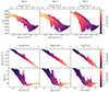 |
Fig. 4. 2D histograms of the characteristics of the halos at the point just before the formation of the first sink particle i.e., when the simulations approached their maximum density, weighted by the total gas mass within each 2D bin. Top panel: temperature-density relation. The collapse is close to isothermal at approximately 8000 K, with the temperature decreasing by only a factor of two over more than ten orders of magnitude in density. Bottom panel: radial profiles of density and H2 abundance. The density-radius relationship follows the ρ ∝ R−2 relationship expected for an isothermal collapse. The H2 abundances are initially negligible at the halo virial radius (R ∼ 100 pc) but increases in the centre of the halo once the density becomes high enough for self-shielding and three-body H2 formation to become effective). |
From the very bottom panel of Fig. 4, the H2 abundance begins to build up, albeit from very low abundance levels, within the inner 10−2 pc (∼2000 au) of the halo. While our LW field strength of J21 = 105 is already quite extreme, we run a second realisation of Halo 3 with an extremely high value of 1010 (as shown in the top panel of Fig. 5) to demonstrate that above roughly 10−15 g cm−3 LW photo-dissociation can not prevent an increase in the H2 abundance (nor probably can any other physical process). The three-body H2 formation rate per unit volume is proportional to n3 (where n is number density), whereas the corresponding scalings for the photodissociation rate and the H2 collisional dissociation rate are n and n2, respectively. Therefore H2 formation will inevitably overcome its destruction at high densities. In practice then the formation of H2 at high densities is inevitable.
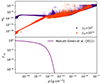 |
Fig. 5. H2 self shielding behaviour. Top: comparison of the build up of H2 in high density regions when a J21 = 105 and 1010 LW radiation field are used. Bottom: H2 shielding factor calculated using Eq. (12) from Wolcott-Green et al. (2011). |
Furthermore, a build in the H2 fraction at high densities owes to the exponential nature of the self-shielding. To demonstrate this, we calculate the H2 shielding factor given in Wolcott-Green et al. (2011) as
where NH2 is the H2 column density. The shielding factor acts as a transmission factor for the LW radiation, with lower values representing more effective shielding. We calculate values of NH2 by extrapolating from the column density-number density power law relation shown in Fig. 3 of Wolcott-Green et al. (2011). The shielding factor is given as a function of density in the bottom panel of Fig. 5, which quickly falls to 00 above densities of 10−15 g cm−3, independently of the LW intensity. This shows that the core will always be shielded from LW radiation above these densities regardless of the value of J21. A build up of H2 fraction within the dense core has been seen to various degrees in the radial profiles of previous studies. For example, the one-zone calculations of Omukai (2001) show a H2 fraction of ∼0.01 at a density of ∼10−8 g cm−3, while simulations by Becerra et al. (2015) reach a H2 fraction of ∼0.1 by ∼10−6 g cm−3 and Regan et al. (2017) reaches a H2 fraction of 10−4 by their maximum density of 10−15 g cm−3. What the results here show is that the very central regions of atomic cooling halos are highly likely to have small pockets of fully molecular gas.
4. Fragmentation and the initial mass function
We now move onto to discuss the build of the initial mass function and the resulting protostellar masses that are found in our simulations at the very highest densities when we introduce sink particles. In Fig. 6 we show the mass flux into concentric shells just before the formation of the first sink particle, comparing the standard Pop III star-forming minihalos (∼106 M⊙) of LP23 with the more massive, atomically cooled halos simulated here. Within the inner ∼100 pc, the accretion rate into the atomic halos exceeds the minihalo case by a factor of between 10 and 1000 due to the combined effects of a stronger DM gravitational well and a larger available reservoir of baryonic gas. In principle this should lead to the formation of more massive sinks given the higher accretion rates possible.
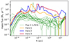 |
Fig. 6. Radial profile of the mass flux through consecutive shells i.e., the accretion rate onto the centre of the halo. For comparison, results from the 15 Pop III star-forming minihalos from LP23 are shown in green. |
Figure 7 shows how the total mass in sink particles, the mass of the most massive sink particle and the total number of sinks evolves in time. The total mass in sinks of the system exceeds the minihalo case by almost 2 order of magnitude due to the higher mass flux. While the initial accretion onto the most massive sink particle far exceeds the same quantity in the minihalos, the most massive sink is ejected from the system, that is, it migrates out of the high density gas and its accretion rate drops to zero in all three atomic halos within the first ∼50 yr after its formation. This results in the most massive sink particle aligning with the upper limit seen in the minihalos. The most surprising result is that the fragmentation of the gas in the centre of the atomic halos far exceeds the minihalo cases.
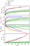 |
Fig. 7. Time evolution of the ratio of the mass of the largest sink to the total mass accreted across all sinks, the mass of the largest sink particle, the total mass accreted onto sink particles, and the total number of sink particles. For comparison, results from the 15 Pop III star-forming minihalos from LP23 are shown in green. |
As discussed earlier, H− formation becomes the dominant cooling process above 10−15 g cm−3, leading to a slightly steeper decline in temperature with density. However, the temperature is still higher in the atomically cooled halos when compared to the minihalo case at the same density (see e.g., Omukai 2000; Yoshida et al. 2006; Prole et al. 2022a), corresponding to a higher Jeans mass. The increase in fragmentation is therefore attributable to the higher mass infall rate. For example, assuming fragmentation is perfectly efficient, the maximum number of fragments that can form is the number of Jeans masses present within the disc. We can therefore get an estimate of the fragmentation from Fig. 8, which shows the number of enclosed Jeans masses of gas at or above a given density. At high densities the number of Jeans masses present in the atomically cooled halos exceeds the minihalo case by an order of magnitude and roughly matches the number of sink particles formed in each halo (see Fig. 7), which explains the increase in fragmentation when compared to the minihalos.
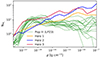 |
Fig. 8. Number of enclosed Jeans masses as a function of density, shown at a time 100 yr after the formation of the first sink particle. The Jeans mass at each density bin is calculated using the mass weighted average temperature and density within the bin. The calculated Jeans mass is then compared to the total mass of gas at or above the density of the bin. |
The combined sink particle mass functions from all three halos are shown in Fig. 9 at ∼100 yr after the formation of the first sink particle. We also show the mass functions from the minihalos at the end of the LP23 simulations (∼300 yr). Despite increased fragmentation and a factor of 3 less in time to accrete, the atomic halo mass function peaks at a higher protostellar mass of 3 M⊙ compared to the 0.3 M⊙ peak in the minihalos. We note that these protostars will continue to accrete for roughly 104 yr before the end of the pre-main sequence. While the zero-age main sequence (ZAMS) masses of these stars are unknown (see Sect. 5), we have confirmed that atomically cooled halos do produce a population of higher mass protostars when compared to regular Pop III star-forming minihalos, at least after the first 100 yr after the formation of the first protostar. These protostars can then accrete the available gas in competition with further star formation.
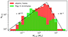 |
Fig. 9. Comparison of the sink particle mass function from the 3 atomic cooling halos at ∼100 yr versus the 15 H2 cooling minihalos from LP23 at ∼300 yr. Power laws of M0.85 and M−2 are superimposed to give the reader an idea of the slopes involved. |
5. Final stellar and black hole masses
In order to estimate the ZAMS masses of the sinks we run lower resolution simulations of Halo 3 which allows us to evolve the system over longer timescales. The top panel of Fig. 10 shows how the total mass of the system of sink particles grows as a function of time across the different resolutions tested. We show the formation of new sink particles in the 10−13 and 10−10 g cm−3 simulations as star shaped markers. We do not show the formation of sinks for the 10−6 g cm−3 cases as fragmentation occurs almost immediately. Clearly the higher the resolution used, the earlier fragmentation occurs. If we take t = 0 to be the time at which the first sink forms in each case then the second sink forms almost immediately in the highest resolution case, after ∼10 yr in the 10−10 g cm−3 case and only after ∼1000 yr in the 10−13 g cm−3 case. As the resolution used does not significantly affect the growth of the total system, the lowest resolution run shows that the system will continue to grow linearly through the pre-main sequence phase to reach a mass of ∼104 M⊙ by 104 yr, that is, there will be ∼104 M⊙ available for star formation within the central 264 au. The increased fragmentation in the higher resolution simulations complicates how this mass will be distributed amongst the protostars. The bottom panel of Fig. 10 shows the accretion rate onto the most massive surviving sink particle, that is, the most massive non-ejected protostar. At the end of the high resolution simulations, the largest survivors in the three halos have accretion rates in the range 10−3–10−1 M⊙ yr−1 and have masses in the range of 7.5–12 M⊙. Among the two lower resolution simulations the final masses of the protostars are approximately 1500 M⊙ (after 1000 years) and 25 000 M⊙ (after 20 000 years) respectively. If the most massive sink particle from the highest resolution simulations can accrete or grow at or near the rates found in the lower resolution simulations then super-massive star formation may be realised.
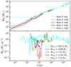 |
Fig. 10. Comparison between the high resolution and low resolution simulations. Top: time evolution of the total mass of the system. The times at which new sink particles formed are indicated with star-shaped markers in the medium and low resolution simulations. We do not show the formation of sink particles for the high resolution simulations as fragmentation occurs almost instantly. Bottom: accretion rates onto the most massive surviving (non-ejected) sink particle. Also shown are the masses of the most massive surviving sink at the end of the simulations. |
The zero-age main sequence (ZAMS) mass of a star depends on the pathway between the formation of the protostar and the eventual beginning of core hydrogen burning, which in turn depends strongly on the evolution of the protostellar accretion rate. When a protostar’s Kelvin–Helmholtz (KH) timescale (time to radiate away its own gravitational energy) is shorter than its accretion timescale (time to double its mass by accretion), it will radiate away its energy and begin to contract, which typically occurs at masses ∼10 M⊙ (Palla & Stahler 1991; Omukai & Palla 2003) though this depends sensitively on the assumed accretion rate (e.g., Nandal et al. 2023). The contraction causes an increased extreme ultraviolet (EUV) luminosity and surface temperature, ionising infalling gas and accelerating it outwards. This triggers a runaway collapse as the decreased accretion rate causes further contraction until hydrogen burning begins and the protostar reaches the ZAMS. If the accretion rate onto the largest sink particle in our high resolution simulations falls and remains below ∼4 × 10⁻³ M⊙ yr−1, the KH contraction will begin at ∼10 M⊙ and the growth of the protostar will be self-regulated by these radiative feedback effects, limiting the final mass to a few tens of M⊙ (Hosokawa et al. 2011, 2012). However, numerous studies have examined the impact that accretion has on the contraction of a Pop III star (e.g., Hirano et al. 2014). A key quantity here is the critical accretion rate – this is the accretion rate onto the stellar surface that prevents contraction of the star. Recently Nandal et al. (2023) investigated in detail this quantity in terms of episodic accretion rates using the Geneva Stellar Evolution code (GENEC: Eggenberger et al. 2008). They found that during the pre-main sequence, which is of most relevance here, the critical accretion rate is ∼2.5 × 10⁻² M⊙ yr−1. Similarly, Herrington et al. (2023) found this critical accretion rate to be 2 × 10⁻² M⊙ yr−1 using the Modules for Experiments in Stellar Astrophysics (MESA: Paxton et al. 2010) code. In this case the effective surface temperature remains below 104 K, hence feedback can not form a H1 region and accretion is not prevented, leading to the formation of a super-giant protostar, which can grow up to several thousand solar masses depending on the details of the accretion (Hosokawa et al. 2013; Umeda et al. 2016; Woods et al. 2017; Haemmerlé et al. 2018; Kimura et al. 2023). This also holds true in the case of episodic accretion (Sakurai et al. 2015, 2016). The end of accretion onto a super-giant protostar is caused by a fast contraction when the accretion rate falls below ∼7 × 10⁻³ M⊙ yr−1.
At the end of the high resolution simulations, the accretion rates onto the largest surviving sink particles vary significantly in time. As the accretion rates onto ∼10 M⊙ protostars appear to be a good indicator of future contraction/accretion evolution (Hosokawa et al. 2011, 2012; Hirano & Bromm 2017) and the largest survivor in Halos 2 and 3 have accretion rates between 10−2 and 10−1 M⊙ yr−1, they could feasibly go on to form (super-massive) Pop III stars with masses anywhere in the range of 10 M⊙ up to 104 M⊙ within their main sequence (MS) lifetime. If they grow in excess of 25 M⊙ the type II supernova explosion would be too weak to eject much of the star and the subsequent fallback of material causes the resulting neutron star to collapse into a BH (MacFadyen et al. 2001), while above 40 M⊙ the neutron star is unable to launch a supernova shock and collapses directly to form a BH with no mass loss (Fryer 1999). If these stars avoid the disruptive pair instability supernova mass ranges of 140–260 M⊙ (Heger & Woosley 2002) and possibly also other supernova islands in the range 2.6–3 × 10⁴ M⊙ (see e.g. Chen et al. 2014; Nagele et al. 2020, 2022), they will result in a massive BH equal in mass to the stellar progenitor. However, whether the protostars will maintain their accretion rates is uncertain. In the optimistic case that they maintain accretion rates of 10−1 M⊙ yr−1, these results are in line with many previous, lower resolution simulations of heavy seed black hole formation (e.g., Johnson et al. 2011; Latif et al. 2013a,d; Regan et al. 2014, 2017; Latif & Volonteri 2015; Choi et al. 2015; Smidt et al. 2018) despite the increased gas fragmentation. The largest survivor in Halo 1 ends with an accretion rate of ∼10−3 M⊙ yr−1, which if maintained will likely lead to an early KH contraction and limit the final mass to 10–30 M⊙. It is unclear if the accretion rate onto Halo 1 will remain below 10−3 or if it will experience an increase similar to that of Halo 3. Certainly the formation of massive BH seeds of 104 M⊙ needed to explain z ∼ 7 quasar observations would rely on frequent mergers with other protostars.
The sink particle masses in the lower resolution simulations represent whole groups of protostars in the high resolution simulations. Frequent mergers of secondary protostars into the main protostar would push the stellar and later BH masses up to close to what is achieved in the low resolution simulations, with an upper limit of 104 M⊙ within a 10 kyr period. These, larger, stellar masses are similar to what studies of atomic cooling cooling haloes by both Regan et al. (2020) and Latif et al. (2022b) have found in their simulations of heavy seed hosting haloes at high-z. However, the issue of unresolved fragmentation is a factor in cosmological simulations with limited dynamic range. In mitigation to this recent studies have pointed out the importance of super competitive accretion, in which a central few stars grow supermassive while a large number of other stars are competing for the gas reservoir (Chon & Omukai 2020), with central objects growing significantly through mergers (Sassano et al. 2021; Vergara et al. 2021; Trinca et al. 2022; Schleicher et al. 2022; Zwick et al. 2023). Here the mass growth by collisions can be comparable to its growth via accretion (Schleicher et al. 2023). The super-competitive accretion scenario was initially invoked to explore the ’low metallicity’ regime (Z ∼ 10−6 − 10−3 Z⊙) where fragmentation is expected to be more active compared to the metal-free case. What we find here is that fragmentation is already vigorous within the central 2000 au of the halo. It therefore appears that for all metallicities below ∼10−3 Z⊙ we can expect a scenario where vigorous fragmentation competes with a rapidly growing protostar. Differentiating the environments which produce a dense stellar cluster versus those that produce a central massive Pop III star may be the next frontier.
To investigate the merger behaviour further, we plot the total number of sink mergers, ratio of total merged mass to accreted sink mass and the ratio of the number of mergers to the number of surviving sink particles as a function of time in Fig. 11. From this we see that the mass gained through mergers constitutes between 1 and 10% of the total sink particle mass. The frequency of mergers is high, with the number of mergers totalling between 10 and 50% of the total number of surviving sink particles. If this holds throughout the following 104 yr, the total mass gained through mergers alone could be as high as 103 M⊙, although it is unclear if this mass would be shared between the growing number of protostars randomly or be preferentially received by the largest growing BH seed.
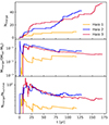 |
Fig. 11. Time evolution of the merger data. Top: cumulative number of sink particle mergers. Middle: ratio of cumulative merged mass to the total accreted sink particle mass (Mtot − M0) where M0 is the initial mass of a sink particle. Bottom: ratio of cumulative number of sink mergers against the current number of surviving sink particles. |
6. Caveats
We have not included magnetic fields in these simulations. While studies of primordial magnetic fields suggest that they can increase the mass of protostars (e.g., Saad et al. 2022; Hirano & Machida 2022; Stacy et al. 2022) and SMBHs (Latif et al. 2013c, 2014), the fields have no effect when they are properly resolved, distributing the magnetic energy from the small-scale turbulent dynamo to smaller spatial scales (Prole et al. 2022b).
We have also not included radiative feedback from our protostars, which has the effect of heating the surrounding gas and lowering accretion rates (e.g., Ardaneh et al. 2018; Luo et al. 2018). While our high resolution simulations end at a point when the protostars would not produce significant levels of feedback, the low resolution simulations run for much longer and would be subject to feedback effects. However, this may not significantly effect the accretion, as Latif et al. (2021) found that radiation from stars and supermassive protostars only reduce the accretion rate onto the central BH by a factor of 2.
In the initial phase of the simulations, we resolved only 4 cells per Jeans length. This has been seen to under resolve turbulent eddies (Federrath et al. 2011) and underestimate small-scale structure and fragmentation (Latif et al. 2013b). However, as previously stated, the initial phase of the simulation was idealised to produce atomically cooled (107 M⊙) halos.
As our high resolution simulations have only captured the first ∼100 yr of accretion after the formation of the first protostar, and the lower resolution simulations lack the capacity to resolve individual star foratmion, to what extent competitive accretion and mergers affect the subsequent final stellar/BH masses is unclear.
Ideally, we would resolve up to the protostellar formation density of 10−4 g cm−3, which is currently computationally unfeasible. Failure to resolve up to that density means we have not achieved numerical convergence. Despite this, our implemented threshold density of 10−6 g cm−3 and post-sink particle run time of 100 yr represents the current state of the art in this regime.
As mentioned in Sect. 2.2, although we account self-consistently for the effects of opacity when computing the H2 cooling rate (due to line cooling and collision-induced emission), we do not yet account for the continuum opacity of the gas when computing the cooling rate due to other radiative processes, for example, H− free-bound cooling. At most densities in our models, the optical depth of the gas in the continuum is small and this simplification has little impact – for example, it should be valid at all of the densities traced in our medium and low resolution models. However, above a density of ∼10−8 g cm−3, we expect the optical depth of the gas in the continuum to become significant, and hence our current simulations over-estimate the cooling rate of the gas above this density. This will likely give us slightly more effective fragmentation at the highest densities than we would find in reality. However, we do not expect this to significantly impact the main conclusions of our study. As Fig. 8 demonstrates, the number of Jeans masses present in the gas at ρ = 10−8 g cm−3 in the atomic cooling halos already substantially exceeds the corresponding value in H2-cooled minihalos, demonstrating that this result is not a consequence of our simplified treatment of very high density cooling. Our finding that the gas fragments extensively in the centre of the atomic-cooled halos should therefore be a robust result, although some of the details (e.g., the precise number of fragments and their formation masses) will depend on the treatment of the cooling at very high densities. Our finding that the fragments quickly grow to become more massive than their Pop III counterparts should also be a robust result: properly accounting for the continuum opacity will likely give us fragments with slightly larger initial masses, which if anything will increase the rate at which they later gain mass, exacerbating the difference between the atomic-cooled and H2-cooled results.
We have assumed that the background radiation field from Pop III stars takes the form of a black body spectrum with an effective temperature of 105 K, peaking in the UV. However, this relies on the stars having masses of ∼300 M⊙ (Schaerer 2002). The masses of Pop III stars are currently uncertain, so our choice of effective temperature affects the photodissociation of the molecules present in the gas. For example, the effective temperature for a 1 M⊙ Pop III star is ∼7000 K (Larkin et al. 2022), which peaks at lower frequencies, resulting in significantly less H2 photodissociating LW radiation but more infrared radiation, which can still photodissociate H− to disrupt H2 formation (Chuzhoy et al. 2007). The methodology here was idealised in that we used a six species chemical model to construct a pristine atomic cooling halo before switching to a full 12 species chemical model and employing an intense LW background. In future work we will apply the same methodology to rapidly assembling halos without the reliance on super-critical LW values.
We have not included radiation contributions from an older or more metal-enriched population of stars as in e.g., Sugimura et al. (2014), Agarwal & Khochfar (2015), Latif et al. (2015), that is, a 104 K black body spectrum peaking at a few eV. We do not expect that a 104 K spectrum would significantly reduce H− abundance in the core, as at the gas densities found in the core, the H− photodissociation rate would be much smaller than the destruction rate of H− by associative detachment (H+H− → H2 + e−) for any reasonable choice of incident radiation field. Furthermore, we do not expect any reduction in the H− abundance to affect the H2 abundance in the core as this only begins to increase beyond densities of 10−15 g cm−3 due to three-body H2 formation, which is independent of the H− abundance.
7. Conclusions
We have performed high resolution simulations of three pristine atomically cooled halos of mass ∼108 M⊙ which begin to collapse at z ∼ 11.5 − 13.3. The goal of our simulation suite was to examine the fragmentation and protostellar formation within the core of such systems as they reach protostellar densities. For the highest resolution we could tractably simulate (ρ ∼ 10−6 g cm−3) we followed the protostar formation for approximately 100 years by introducing sink particles representing individual protostars. The main results are as follows:
-
Resolving protostellar densities reveals that the centre of (pristine) atomically cooled halos is subject to intense fragmentation, even more-so than in the canonical Pop III minihalo case. This is driven by H− free-bound cooling and an increased number of Jeans masses within the core, owing to enhanced accretion rates.
-
Despite increased fragmentation, the atomically cooled halos formed a population of higher mass protostars compared to Pop III star-forming minihalos.
-
The initial accretion rates onto the most massive surviving protostars indicates that their zero-age main sequence masses could range from 102 to 104 M⊙ depending on subsequent accretion and/or mergers.
-
Our coarser resolution simulations show that the total mass of the system continues to grow steadily for at least 104 years after the formation of the first protostar (achieving central sink particle masses in excess of 104 M⊙), although how this is distributed amongst the rapidly growing number of protostars is unknown and requires further study.
-
The formation of a massive Pop III star (M* ≳ 1000 M⊙) is therefore realistic and achievable in a high-z setting but relies on (super-competitive) accretion and frequent mergers with secondary protostars
-
The H2 fraction within the inner ∼2000 au of all three halos was able to build up independently of the strength of the external LW radiation field. This strongly indicates that all collapsing halos (even those subject to strong LW fields and likely other physical processes which could suppress star formation up to the atomic limit e.g., streaming velocities between DM and baryonic gas) contain small pockets of cold, H2 rich gas at their centre.
The findings here show that the formation of massive Pop III stars (i.e., heavy seed MBHs) is entirely plausible in sufficiently massive halos but will depend sensitively on the future evolution of the protostars and on the balance between stellar accretion and mergers in the dense cluster that forms within the centre of the atomic cooling halo. While we model the impact of a super-critical LW radiation field here, any physical process which results in the initial suppression of star formation up to the atomic cooling limit should have a similar impact and allow for the formation of more massive Pop III stars.
Acknowledgments
LP and JR acknowledge support from the Irish Research Council Laureate programme under grant number IRCLA/2022/1165. JR also acknowledges support from the Royal Society and Science Foundation Ireland under grant number URF/R1/191132. This work used the DiRAC@Durham facility managed by the Institute for Computational Cosmology on behalf of the STFC DiRAC HPC Facility (www.dirac.ac.uk). The equipment was funded by BEIS capital funding via STFC capital grants ST/P002293/1, ST/R002371/1 and ST/S002502/1, Durham University and STFC operations grant ST/R000832/1. DiRAC is part of the National e-Infrastructure. We also acknowledge the support of the Supercomputing Wales project, which is part-funded by the European Regional Development Fund (ERDF) via Welsh Government. SCOG and RSK acknowledge financial support from the European Research Council via the ERC Synergy Grant ECOGAL (project ID 855130), from the Heidelberg Cluster of Excellence (EXC 2181 – 390900948) “STRUCTURES”, funded by the German Excellence Strategy, and by the German Ministry for Economic Affairs and Climate Action in project “MAINN” (funding ID 50OO2206). They also thank for computing resources provided by the Ministry of Science, Research and the Arts (MWK) of the State of Baden-Württemberg and Deutsche Forschungsgemeinschaft (DFG) through grant INST 35/1134-1 FUGG and for data storage at SDS@hd through grant INST 35/1314-1 FUGG. Finally, we acknowledge Advanced Research Computing at Cardiff (ARCCA) for providing resources for the project.
References
- Abel, T., Anninos, P., Zhang, Y., & Norman, M. L. 1997, New Astron., 2, 181 [NASA ADS] [CrossRef] [Google Scholar]
- Abel, T., Bryan, G. L., & Norman, M. L. 2002, Science, 295, 93 [CrossRef] [Google Scholar]
- Agarwal, B., & Khochfar, S. 2015, MNRAS, 446, 160 [CrossRef] [Google Scholar]
- Agarwal, B., Smith, B., Glover, S., Natarajan, P., & Khochfar, S. 2016, MNRAS, 459, 4209 [NASA ADS] [CrossRef] [Google Scholar]
- Alexander, T., & Natarajan, P. 2014, Science, 345, 1330 [NASA ADS] [CrossRef] [Google Scholar]
- Alvarez, M. A., Wise, J. H., & Abel, T. 2009, ApJ, 701, L133 [NASA ADS] [CrossRef] [Google Scholar]
- Arca Sedda, M., Mapelli, M., Benacquista, M., & Spera, M. 2023, MNRAS, 520, 5259 [NASA ADS] [CrossRef] [Google Scholar]
- Ardaneh, K., Luo, Y., Shlosman, I., et al. 2018, MNRAS, 479, 2277 [NASA ADS] [CrossRef] [Google Scholar]
- Becerra, F., Greif, T. H., Springel, V., & Hernquist, L. E. 2015, MNRAS, 446, 2380 [NASA ADS] [CrossRef] [Google Scholar]
- Becerra, F., Marinacci, F., Bromm, V., & Hernquist, L. E. 2018a, MNRAS, 480, 5029 [NASA ADS] [Google Scholar]
- Becerra, F., Marinacci, F., Inayoshi, K., Bromm, V., & Hernquist, L. E. 2018b, ApJ, 857, 138 [NASA ADS] [CrossRef] [Google Scholar]
- Beckmann, R. S., Dubois, Y., Guillard, P., et al. 2019, A&A, 631, A60 [EDP Sciences] [Google Scholar]
- Berger, M. J., & Colella, P. 1989, J. Comput. Phys., 82, 64 [CrossRef] [Google Scholar]
- Boekholt, T. C. N., Schleicher, D. R. G., Fellhauer, M., et al. 2018, MNRAS, 476, 366 [Google Scholar]
- Bromm, V., & Loeb, A. 2003, ApJ, 596, 34 [Google Scholar]
- Bromm, V., & Yoshida, N. 2011, ARA&A, 49, 373 [CrossRef] [Google Scholar]
- Bromm, V., Coppi, P. S., & Larson, R. B. 1999, ApJ, 527, L5 [NASA ADS] [CrossRef] [PubMed] [Google Scholar]
- Bromm, V., Kudritzki, R. P., & Loeb, A. 2001, ApJ, 552, 464 [NASA ADS] [CrossRef] [Google Scholar]
- Chen, K.-J., Heger, A., Woosley, S., et al. 2014, ApJ, 790, 162 [CrossRef] [Google Scholar]
- Choi, J.-H., Shlosman, I., & Begelman, M. C. 2015, MNRAS, 450, 4411 [NASA ADS] [CrossRef] [Google Scholar]
- Chon, S., & Omukai, K. 2020, MNRAS, 494, 2851 [Google Scholar]
- Chon, S., Hirano, S., Hosokawa, T., & Yoshida, N. 2016, ApJ, 832, 134 [NASA ADS] [CrossRef] [Google Scholar]
- Chon, S., Hosokawa, T., & Yoshida, N. 2018, MNRAS, 475, 4104 [CrossRef] [Google Scholar]
- Chuzhoy, L., Kuhlen, M., & Shapiro, P. R. 2007, ApJ, 665, L85 [NASA ADS] [CrossRef] [Google Scholar]
- Clark, P. C., Glover, S. C. O., Smith, R. J., et al. 2011, Science, 331, 1040 [Google Scholar]
- Clark, P. C., Glover, S. C. O., & Klessen, R. S. 2012, MNRAS, 420, 745 [NASA ADS] [CrossRef] [Google Scholar]
- Dong, F., Zhao, D., Han, J., et al. 2022, ApJ, 929, 120 [NASA ADS] [CrossRef] [Google Scholar]
- Dunn, G., Bellovary, J., Holley-Bockelmann, K., Christensen, C., & Quinn, T. 2018, ApJ, 861, 39 [CrossRef] [Google Scholar]
- Eggenberger, P., Meynet, G., Maeder, A., et al. 2008, Astrophys. Space Sci., 316, 43 [NASA ADS] [CrossRef] [Google Scholar]
- Eisenstein, D. J., & Hu, W. 1998, ApJ, 496, 605 [Google Scholar]
- Fan, X., Banados, E., Simcoe, A. R., 2023, ARA&A, 61, 373 [NASA ADS] [CrossRef] [Google Scholar]
- Federrath, C., Sur, S., Schleicher, D. R. G., Banerjee, R., & Klessen, R. S. 2011, ApJ, 731, 62 [NASA ADS] [CrossRef] [Google Scholar]
- Fernandez, R., Bryan, G. L., Haiman, Z., & Li, M. 2014, MNRAS, 439, 3798 [CrossRef] [Google Scholar]
- Field, G. B., Somerville, W. B., & Dressler, K. 1966, ARA&A, 4, 207 [NASA ADS] [CrossRef] [Google Scholar]
- Fryer, C. L. 1999, ApJ, 522, 413 [NASA ADS] [CrossRef] [Google Scholar]
- Glebbeek, E., Gaburov, E., de Mink, S. E., Pols, O. R., & Zwart, S. F. P. 2009, A&A, 497, 255 [NASA ADS] [CrossRef] [EDP Sciences] [Google Scholar]
- Glover, S. C. O. 2015, MNRAS, 451, 2082 [NASA ADS] [CrossRef] [Google Scholar]
- Glover, S. C. O., & Abel, T. 2008, MNRAS, 388, 1627 [NASA ADS] [CrossRef] [Google Scholar]
- Glover, S. C., Savin, D. W., & Jappsen, A.-K. 2006, ApJ, 640, 553 [NASA ADS] [CrossRef] [Google Scholar]
- Greif, T. H., Johnson, J. L., Klessen, R. S., & Bromm, V. 2008, MNRAS, 387, 1021 [NASA ADS] [CrossRef] [Google Scholar]
- Greif, T. H., Bromm, V., Clark, P. C., et al. 2012, MNRAS, 424, 399 [NASA ADS] [CrossRef] [Google Scholar]
- Haemmerlé, L., Woods, T. E., Klessen, R. S., Heger, A., & Whalen, D. J. 2018, MNRAS, 474, 2757 [Google Scholar]
- Hahn, O., & Abel, T. 2011, MNRAS, 415, 2101 [Google Scholar]
- Haiman, Z., Thoul, A. A., & Loeb, A. 1996, ApJ, 464, 523 [NASA ADS] [CrossRef] [Google Scholar]
- Haiman, Z., Rees, M. J., & Loeb, A. 1997, ApJ, 476, 458 [NASA ADS] [CrossRef] [Google Scholar]
- Haiman, Z., Abel, T., & Rees, M. J. 2000, ApJ, 534, 11 [NASA ADS] [CrossRef] [Google Scholar]
- Hartwig, T., Glover, S. C. O., Klessen, R. S., Latif, M. A., & Volonteri, M. 2015, MNRAS, 452, 1233 [NASA ADS] [CrossRef] [Google Scholar]
- Heger, A., & Woosley, S. E. 2002, ApJ, 567, 532 [Google Scholar]
- Heitmann, K., Lukić, Z., Fasel, P., et al. 2008, Computat. Sci. Discov., 1, 015003 [NASA ADS] [CrossRef] [Google Scholar]
- Herrington, N. P., Whalen, D. J., & Woods, T. E. 2023, MNRAS, 521, 463 [CrossRef] [Google Scholar]
- Hirano, S., & Bromm, V. 2017, MNRAS, 470, 898 [CrossRef] [Google Scholar]
- Hirano, S., & Machida, M. N. 2022, ApJ, 935, L16 [NASA ADS] [CrossRef] [Google Scholar]
- Hirano, S., Hosokawa, T., Yoshida, N., et al. 2014, ApJ, 781, 60 [NASA ADS] [CrossRef] [Google Scholar]
- Hosokawa, T., & Omukai, K. 2009, ApJ, 691, 823 [Google Scholar]
- Hosokawa, T., Omukai, K., Yoshida, N., & Yorke, H. W. 2011, Science, 334, 1250 [CrossRef] [Google Scholar]
- Hosokawa, T., Omukai, K., & Yorke, H. W. 2012, ApJ, 756, 93 [Google Scholar]
- Hosokawa, T., Yorke, H. W., Inayoshi, K., Omukai, K., & Yoshida, N. 2013, ApJ, 778, 178 [Google Scholar]
- Huang, K.-W., Di Matteo, T., Bhowmick, A. K., Feng, Y., & Ma, C.-P. 2018, MNRAS, 478, 5063 [CrossRef] [Google Scholar]
- Inayoshi, K., Omukai, K., & Tasker, E. 2014, MNRAS, 445, L109 [NASA ADS] [CrossRef] [Google Scholar]
- Inayoshi, K., Haiman, Z., & Ostriker, J. P. 2016, MNRAS, 459, 3738 [NASA ADS] [CrossRef] [Google Scholar]
- Johnson, J. L., & Bromm, V. 2007, MNRAS, 374, 1557 [NASA ADS] [CrossRef] [Google Scholar]
- Johnson, J. L., Khochfar, S., Greif, T. H., & Durier, F. 2011, MNRAS, 410, 919 [NASA ADS] [CrossRef] [Google Scholar]
- Katz, H., Sijacki, D., & Haehnelt, M. G. 2015, MNRAS, 451, 2352 [Google Scholar]
- Kimura, K., Hosokawa, T., Sugimura, K., & Fukushima, H. 2023, ApJ, 950, 184 [NASA ADS] [CrossRef] [Google Scholar]
- Klessen, R. S., & Glover, S. C. O. 2023, ARA&A, 61, 65 [NASA ADS] [CrossRef] [Google Scholar]
- Larkin, M. M., Gerasimov, R., & Burgasser, A. J. 2022, AJ, 165, 2 [Google Scholar]
- Latif, M. A., & Volonteri, M. 2015, MNRAS, 452, 1026 [CrossRef] [Google Scholar]
- Latif, M. A., Schleicher, D. R. G., Schmidt, W., & Niemeyer, J. 2013a, MNRAS, 433, 1607 [NASA ADS] [CrossRef] [Google Scholar]
- Latif, M. A., Schleicher, D. R. G., Schmidt, W., & Niemeyer, J. 2013b, MNRAS, 430, 588 [NASA ADS] [CrossRef] [Google Scholar]
- Latif, M. A., Schleicher, D. R. G., Schmidt, W., & Niemeyer, J. 2013c, MNRAS, 432, 668 [NASA ADS] [CrossRef] [Google Scholar]
- Latif, M. A., Schleicher, D. R. G., Schmidt, W., & Niemeyer, J. C. 2013d, MNRAS, 436, 2989 [Google Scholar]
- Latif, M. A., Schleicher, D. R. G., & Schmidt, W. 2014, MNRAS, 440, 1551 [CrossRef] [Google Scholar]
- Latif, M. A., Bovino, S., Grassi, T., Schleicher, D. R. G., & Spaans, M. 2015, MNRAS, 446, 3163 [CrossRef] [Google Scholar]
- Latif, M. A., Khochfar, S., & Whalen, D. 2020, ApJ, 892, L4 [NASA ADS] [CrossRef] [Google Scholar]
- Latif, M. A., Khochfar, S., Schleicher, D., & Whalen, D. J. 2021, MNRAS, 508, 1756 [NASA ADS] [CrossRef] [Google Scholar]
- Latif, M. A., Whalen, D., & Khochfar, S. 2022a, ApJ, 925, 28 [NASA ADS] [CrossRef] [Google Scholar]
- Latif, M. A., Whalen, D. J., Khochfar, S., Herrington, N. P., & Woods, T. E. 2022b, Nature, 607, 48 [CrossRef] [Google Scholar]
- Loeb, A., & Rasio, F. A. 1994, ApJ, 432, 52 [Google Scholar]
- Luo, Y., Ardaneh, K., Shlosman, I., et al. 2018, MNRAS, 476, 3523 [CrossRef] [Google Scholar]
- Lupi, A., Haardt, F., Dotti, M., et al. 2016, MNRAS, 456, 2993 [NASA ADS] [CrossRef] [Google Scholar]
- MacFadyen, A. I., Woosley, S. E., & Heger, A. 2001, ApJ, 550, 410 [NASA ADS] [CrossRef] [Google Scholar]
- Machida, M. N., & Nakamura, T. 2015, MNRAS, 448, 1405 [NASA ADS] [CrossRef] [Google Scholar]
- Massonneau, W., Volonteri, M., Dubois, Y., & Beckmann, R. S. 2023, A&A, 670, A180 [NASA ADS] [CrossRef] [EDP Sciences] [Google Scholar]
- Matsuoka, Y., Onoue, M., Kashikawa, N., et al. 2019, ApJ, 872, L2 [Google Scholar]
- Mayer, L., & Bonoli, S. 2018, Rep. Progr. Phys., 82, 016901 [Google Scholar]
- Mayer, L., Kazantzidis, S., Escala, A., & Callegari, S. 2010, Nature, 466, 1082 [Google Scholar]
- Micic, M., Holley-Bockelmann, K., Sigurdsson, S., & Abel, T. 2007, MNRAS, 380, 1533 [CrossRef] [Google Scholar]
- Milosavljević, M., Couch, S. M., & Bromm, V. 2009, ApJ, 696, L146 [CrossRef] [Google Scholar]
- Monaghan, J. J. 1992, ARA&A, 30, 543 [NASA ADS] [CrossRef] [Google Scholar]
- Mortlock, D. J., Warren, S. J., Venemans, B. P., et al. 2011, Nature, 474, 616 [Google Scholar]
- Nagele, C., Umeda, H., Takahashi, K., Yoshida, T., & Sumiyoshi, K. 2020, MNRAS, 496, 1224 [NASA ADS] [CrossRef] [Google Scholar]
- Nagele, C., Umeda, H., Takahashi, K., Yoshida, T., & Sumiyoshi, K. 2022, MNRAS, 517, 1584 [NASA ADS] [CrossRef] [Google Scholar]
- Nakamura, F., & Umemura, M. 2002, ApJ, 569, 549 [NASA ADS] [CrossRef] [Google Scholar]
- Nandal, D., Regan, J. A., Woods, T. E., et al. 2023, A&A, 677, A155 [NASA ADS] [CrossRef] [EDP Sciences] [Google Scholar]
- Oh, S. P., & Haiman, Z. 2002, ApJ, 569, 558 [NASA ADS] [CrossRef] [Google Scholar]
- Omukai, K. 2000, ApJ, 534, 809 [NASA ADS] [CrossRef] [Google Scholar]
- Omukai, K. 2001, ApJ, 546, 635 [NASA ADS] [CrossRef] [Google Scholar]
- Omukai, K., & Palla, F. 2003, ApJ, 589, 677 [NASA ADS] [CrossRef] [Google Scholar]
- Palla, F., & Stahler, W. S. 1991, ApJ, 375, 288 [NASA ADS] [CrossRef] [Google Scholar]
- Patrick, S. J., Whalen, D. J., Elford, J. S., & Latif, M. A. 2023, MNRAS, 522, 3795 [NASA ADS] [CrossRef] [Google Scholar]
- Paxton, B., Bildsten, L., Dotter, A., et al. 2010, ApJS, 192, 3 [Google Scholar]
- Pfister, H., Volonteri, M., Dubois, Y., Dotti, M., & Colpi, M. 2019, MNRAS, 486, 101 [Google Scholar]
- Planck Collaboration VI. 2020, A&A, 641, A6 [NASA ADS] [CrossRef] [EDP Sciences] [Google Scholar]
- Portegies Zwart, S. F., Baumgardt, H., Hut, P., Makino, J., & McMillan, S. L. W. 2004, Nature, 428, 724 [Google Scholar]
- Prieto, J., Jimenez, R., & Haiman, Z. 2013, MNRAS, 436, 2301 [NASA ADS] [CrossRef] [Google Scholar]
- Prole, L. R., Clark, P. C., Klessen, R. S., & Glover, S. C. O. 2022a, MNRAS, 510, 4019 [NASA ADS] [CrossRef] [Google Scholar]
- Prole, L. R., Clark, P. C., Klessen, R. S., Glover, S. C. O., & Pakmor, R. 2022b, MNRAS, 516, 2223 [NASA ADS] [CrossRef] [Google Scholar]
- Prole, L. R., Schauer, A. T. P., Clark, P. C., et al. 2023, MNRAS, 520, 2081 [NASA ADS] [CrossRef] [Google Scholar]
- Ptak, A., & Colbert, E. 2004, ApJ, 606, 291 [CrossRef] [Google Scholar]
- Rees, M. J. 1978, Phys. Scr., 17, 193 [NASA ADS] [CrossRef] [Google Scholar]
- Regan, J. A., & Haehnelt, M. G. 2009, MNRAS, 396, 343 [CrossRef] [Google Scholar]
- Regan, J. A., Johansson, P. H., & Wise, J. H. 2014, ApJ, 795, 137 [NASA ADS] [CrossRef] [Google Scholar]
- Regan, J. A., Visbal, E., Wise, J. H., et al. 2017, Nat. Astron., 1, 1 [Google Scholar]
- Regan, J. A., Downes, T. P., Volonteri, M., et al. 2019, MNRAS, 486, 3892 [CrossRef] [Google Scholar]
- Regan, J. A., Wise, J. H., Woods, T. E., et al. 2020, Open J. Astrophys., 3 [Google Scholar]
- Regan, J. A., Pacucci, F., & Bustamante-Rosell, M. J. 2023, MNRAS, 518, 5997 [Google Scholar]
- Reinoso, B., Klessen, R. S., Schleicher, D., Glover, S. C. O., & Solar, P. 2023, MNRAS, 521, 3553 [CrossRef] [Google Scholar]
- Saad, C. R., Bromm, V., & El Eid, M. 2022, MNRAS, 516, 3130 [NASA ADS] [CrossRef] [Google Scholar]
- Sakurai, Y., Hosokawa, T., Yoshida, N., & Yorke, H. W. 2015, MNRAS, 452, 755 [Google Scholar]
- Sakurai, Y., Vorobyov, E. I., Hosokawa, T., et al. 2016, MNRAS, 459, 1137 [NASA ADS] [CrossRef] [Google Scholar]
- Sassano, F., Schneider, R., Valiante, R., et al. 2021, MNRAS, 506, 613 [CrossRef] [Google Scholar]
- Schaerer, D. 2002, A&A, 382, 28 [NASA ADS] [CrossRef] [EDP Sciences] [Google Scholar]
- Schauer, A. T. P., Glover, S. C. O., Klessen, R. S., & Ceverino, D. 2019, MNRAS, 484, 3510 [NASA ADS] [CrossRef] [Google Scholar]
- Schleicher, D. R. G., Reinoso, B., Latif, M., et al. 2022, MNRAS, 512, 6192 [NASA ADS] [CrossRef] [Google Scholar]
- Schleicher, D. R. G., Reinoso, B., & Klessen, R. S. 2023, MNRAS, 521, 3972 [NASA ADS] [CrossRef] [Google Scholar]
- Shang, C., Bryan, G. L., & Haiman, Z. 2010, MNRAS, 402, 1249 [NASA ADS] [CrossRef] [Google Scholar]
- Smidt, J., Whalen, D. J., Johnson, J. L., Surace, M., & Li, H. 2018, ApJ, 865, 126 [NASA ADS] [CrossRef] [Google Scholar]
- Smith, R. J., Glover, S. C. O., Clark, P. C., Greif, T., & Klessen, R. S. 2011, MNRAS, 414, 3633 [NASA ADS] [CrossRef] [Google Scholar]
- Smith, B. D., Regan, J. A., Downes, T. P., et al. 2018, MNRAS, 480, 3762 [NASA ADS] [CrossRef] [Google Scholar]
- Spaans, M., & Silk, J. 2006, ApJ, 652, 902 [NASA ADS] [CrossRef] [Google Scholar]
- Springel, V. 2010, MNRAS, 401, 791 [Google Scholar]
- Stacy, A., Greif, T. H., & Bromm, V. 2010, MNRAS, 403, 45 [NASA ADS] [CrossRef] [Google Scholar]
- Stacy, A., McKee, C. F., Lee, A. T., Klein, R. I., & Li, P. S. 2022, MNRAS, 511, 5042 [NASA ADS] [CrossRef] [Google Scholar]
- Stecher, T. P., & Williams, D. A. 1967, ApJ, 149, L29 [NASA ADS] [CrossRef] [Google Scholar]
- Stone, N. C., Küpper, A. H. W., & Ostriker, J. P. 2017, MNRAS, 467, 4180 [NASA ADS] [Google Scholar]
- Su, K.-Y., Bryan, G. L., Haiman, Z., et al. 2023, MNRAS, 520, 4258 [NASA ADS] [CrossRef] [Google Scholar]
- Suazo, M., Prieto, J., Escala, A., & Schleicher, D. R. G. 2019, ApJ, 885, 127 [NASA ADS] [CrossRef] [Google Scholar]
- Sugimura, K., Omukai, K., & Inoue, A. K. 2014, MNRAS, 445, 544 [NASA ADS] [CrossRef] [Google Scholar]
- Susa, H. 2019, ApJ, 877, 99 [NASA ADS] [CrossRef] [Google Scholar]
- Tegmark, M., Silk, J., Rees, M. J., et al. 1997, ApJ, 474, 1 [NASA ADS] [CrossRef] [Google Scholar]
- Tenneti, A., Di Matteo, T., Croft, R., Garcia, T., & Feng, Y. 2018, MNRAS, 474, 597 [CrossRef] [Google Scholar]
- Tress, R. G., Smith, R. J., Sormani, M. C., et al. 2020, MNRAS, 492, 2973 [Google Scholar]
- Trinca, A., Schneider, R., Valiante, R., et al. 2022, MNRAS, 511, 616 [NASA ADS] [CrossRef] [Google Scholar]
- Truelove, J. K., Klein, R. I., McKee, C. F., et al. 1997, ApJ, 489, L179 [CrossRef] [Google Scholar]
- Turk, M. J., Clark, P., Glover, S. C. O., et al. 2011, ApJ, 726, 726 [Google Scholar]
- Umeda, H., Hosokawa, T., Omukai, K., & Yoshida, N. 2016, ApJ, 830, L34 [Google Scholar]
- Vergara, M. Z. C., Schleicher, D. R. G., Boekholt, T. C. N., et al. 2021, A&A, 649, A160 [NASA ADS] [CrossRef] [EDP Sciences] [Google Scholar]
- Wise, J. H., Regan, J. A., O’Shea, B. W., et al. 2019, Nature, 566, 85 [NASA ADS] [CrossRef] [Google Scholar]
- Wolcott-Green, J., Haiman, Z., & Bryan, G. L. 2011, MNRAS, 418, 838 [NASA ADS] [CrossRef] [Google Scholar]
- Wollenberg, K. M. J., Glover, S. C. O., Clark, P. C., & Klessen, R. S. 2020, MNRAS, 494, 1871 [NASA ADS] [CrossRef] [Google Scholar]
- Woods, T. E., Heger, A., Whalen, D. J., Haemmerlé, L., & Klessen, R. S. 2017, ApJ, 842, L6 [Google Scholar]
- Woods, T. E., Heger, A., & Haemmerlé, L. 2020, MNRAS, 494, 2236 [Google Scholar]
- Yoshida, N., Omukai, K., Hernquist, L., & Abel, T. 2006, ApJ, 652, 6 [NASA ADS] [CrossRef] [Google Scholar]
- Yoshida, N., Omukai, K., & Hernquist, L. 2007, ApJ, 667, L117 [NASA ADS] [CrossRef] [Google Scholar]
- Zhu, Q., Li, Y., Li, Y., et al. 2022, MNRAS, 514, 5583 [NASA ADS] [CrossRef] [Google Scholar]
- Zwick, L., Mayer, L., Haemmerlé, L., & Klessen, R. S. 2023, MNRAS, 518, 2076 [Google Scholar]
All Tables
Halo virial masses, radii, and temperatures along with redshifts at the point where they were extracted from the initial cosmological simulation.
All Figures
|
Fig. 1. 2D histograms of the temperature – density profiles for the halos at the point at which they were extracted from the initial cosmological simulation, weighted by total gas mass within each 2D bin. The halos have begun to gravitationally collapse via atomic cooling as seen from the close to isothermal temperature profile. They differ from the regular H2 minihalo case by the absence of a sharp drop in temperature to ∼200 K beginning at ∼10−23 g cm−3. |
| In the text | |
|
Fig. 2. Radial profiles of enclosed gas and DM mass for the three atomic halos at the point where they were extracted from the initial cosmological simulation. The baryonic component becomes comparable to the DM within the central ∼100 pc where it begins to decouple from the DM. In Halo 3, the baryonic component is dominant over DM on these scales. |
| In the text | |
|
Fig. 3. Projection images of the zoom-in simulation box, showing density, H2 fraction and temperature for Halo 3 at the end of the simulation. From left to right, the zoom-in plots show at radius of 1 kpc, 10 pc and 0.1 pc, respectively. |
| In the text | |
|
Fig. 4. 2D histograms of the characteristics of the halos at the point just before the formation of the first sink particle i.e., when the simulations approached their maximum density, weighted by the total gas mass within each 2D bin. Top panel: temperature-density relation. The collapse is close to isothermal at approximately 8000 K, with the temperature decreasing by only a factor of two over more than ten orders of magnitude in density. Bottom panel: radial profiles of density and H2 abundance. The density-radius relationship follows the ρ ∝ R−2 relationship expected for an isothermal collapse. The H2 abundances are initially negligible at the halo virial radius (R ∼ 100 pc) but increases in the centre of the halo once the density becomes high enough for self-shielding and three-body H2 formation to become effective). |
| In the text | |
|
Fig. 5. H2 self shielding behaviour. Top: comparison of the build up of H2 in high density regions when a J21 = 105 and 1010 LW radiation field are used. Bottom: H2 shielding factor calculated using Eq. (12) from Wolcott-Green et al. (2011). |
| In the text | |
|
Fig. 6. Radial profile of the mass flux through consecutive shells i.e., the accretion rate onto the centre of the halo. For comparison, results from the 15 Pop III star-forming minihalos from LP23 are shown in green. |
| In the text | |
|
Fig. 7. Time evolution of the ratio of the mass of the largest sink to the total mass accreted across all sinks, the mass of the largest sink particle, the total mass accreted onto sink particles, and the total number of sink particles. For comparison, results from the 15 Pop III star-forming minihalos from LP23 are shown in green. |
| In the text | |
|
Fig. 8. Number of enclosed Jeans masses as a function of density, shown at a time 100 yr after the formation of the first sink particle. The Jeans mass at each density bin is calculated using the mass weighted average temperature and density within the bin. The calculated Jeans mass is then compared to the total mass of gas at or above the density of the bin. |
| In the text | |
|
Fig. 9. Comparison of the sink particle mass function from the 3 atomic cooling halos at ∼100 yr versus the 15 H2 cooling minihalos from LP23 at ∼300 yr. Power laws of M0.85 and M−2 are superimposed to give the reader an idea of the slopes involved. |
| In the text | |
|
Fig. 10. Comparison between the high resolution and low resolution simulations. Top: time evolution of the total mass of the system. The times at which new sink particles formed are indicated with star-shaped markers in the medium and low resolution simulations. We do not show the formation of sink particles for the high resolution simulations as fragmentation occurs almost instantly. Bottom: accretion rates onto the most massive surviving (non-ejected) sink particle. Also shown are the masses of the most massive surviving sink at the end of the simulations. |
| In the text | |
|
Fig. 11. Time evolution of the merger data. Top: cumulative number of sink particle mergers. Middle: ratio of cumulative merged mass to the total accreted sink particle mass (Mtot − M0) where M0 is the initial mass of a sink particle. Bottom: ratio of cumulative number of sink mergers against the current number of surviving sink particles. |
| In the text | |
Current usage metrics show cumulative count of Article Views (full-text article views including HTML views, PDF and ePub downloads, according to the available data) and Abstracts Views on Vision4Press platform.
Data correspond to usage on the plateform after 2015. The current usage metrics is available 48-96 hours after online publication and is updated daily on week days.
Initial download of the metrics may take a while.