| Issue |
A&A
Volume 684, April 2024
|
|
|---|---|---|
| Article Number | A125 | |
| Number of page(s) | 16 | |
| Section | The Sun and the Heliosphere | |
| DOI | https://doi.org/10.1051/0004-6361/202348703 | |
| Published online | 11 April 2024 | |
Sliding-window cross-correlation and mutual information methods in the analysis of solar wind measurements
Institute of Experimental and Applied Physics, Christian-Albrechts-University Kiel, Leibnizstraße 11, 24118 Kiel, Germany
e-mail: This email address is being protected from spambots. You need JavaScript enabled to view it.
Received:
22
November
2023
Accepted:
30
January
2024
Abstract
Context. When describing the relationships between two data sets, four crucial aspects must be considered, namely: timescales, intrinsic lags, linear relationships, and non-linear relationships. We present a tool that combines these four aspects and visualizes the underlying structure where two data sets are highly related. The basic mathematical methods used here are cross-correlation and mutual information (MI) analyses. As an example, we applied these methods to a set of two-month’s worth of solar wind density and total magnetic field strength data.
Aims. Two neighboring solar wind parcels may have undergone different heating and acceleration processes and may even originate from different source regions. However, they may share very similar properties, which would effectively “hide” their different origins. When this hidden information is mixed with noise, describing the relationships between two solar wind parameters becomes challenging. Time lag effects and non-linear relationships between solar wind parameters are often overlooked, while simple time-lag-free linear relationships are sometimes insufficient to describe the complex processes in space physics. Thus, we propose this tool to analyze the monotonic (or linear) and non-monotonic (or non-linear) relationships between a pair of solar wind parameters within a certain time period, taking into consideration the effects of different timescales and possible time lags.
Methods. Our tool consists of two parts: the sliding-window cross-correlation (SWCC) method and sliding-window mutual information (SWMI) method. As their names suggest, both parts involve a set of sliding windows. By independently sliding these windows along the time axis of the two time series, this technique can assess the correlation coefficient (and mutual information) between any two windowed data sets with any time lags. Visualizing the obtained results enables us to identify structures where two time series are highly correlated, while providing information on the relevant timescales and time lags.
Results. We applied our proposed tool to solar wind density and total magnetic field strength data. Structures with distinct timescales were identified. Our tool also detected the presence of short-term anti-correlations coexisting with long-term positive correlations between solar wind density and magnetic field strength. Some non-monotonic relationships were also found.
Conclusions. The visual products of our tool (the SWCC+SWMI maps) represent an innovative extension of traditional numerical methods, offering users a more intuitive perspective on the data. The SWCC and SWMI methods can be used to identify time periods where one parameter has a strong influence on the other. Of course, they can also be applied to other data, such as multi-wavelength photometric and spectroscopic time series, thus providing a new tool for solar physics analyses.
Key words: methods: data analysis / solar wind
© The Authors 2024
 Open Access article, published by EDP Sciences, under the terms of the Creative Commons Attribution License (https://creativecommons.org/licenses/by/4.0), which permits unrestricted use, distribution, and reproduction in any medium, provided the original work is properly cited.
This article is published in open access under the Subscribe to Open model. This email address is being protected from spambots. You need JavaScript enabled to view it. to support open access publication.
1. Introduction
The correlation between two data sets is often used to analyze possible relationships between them. Time series are very common data products of solar wind measurements and different time series generally have different inherent timescales; thus, timescales play an important role when the correlation between two time series is discussed.
On long timescales, the proton temperature is positively correlated with the solar wind speed (Marsch et al. 1982; D’Amicis et al. 2019) at 1 AU; the O7+/O6+ is anti-correlated with solar wind speed (Geiss et al. 1995a; Kasper et al. 2012; Zhao et al. 2009); and the elemental abundance Mg/O and O7+/O6+ ratios are well correlated (Geiss et al. 1995a). More recently the electron temperature was confirmed to have a strong negative correlation with the solar wind speed (Marsch et al. 1989; Maksimovic et al. 2020; Shi et al. 2023) at a closer distance. However, the timescale does matter. Correlations derived from long time series of long-term averages could significantly differ within short time intervals (Marubashi 1995; Asbridge et al. 1976; Barrow 1978). Short-term correlations also have the potential to provide insights that may be concealed by long-term trends (Georgieva et al. 2007; Simms et al. 2022).
All correlations mentioned above are based on a related correlation coefficient (cc), for instance, the Pearson cc (Benesty et al. 2009; De Winter et al. 2016), which quantifies linear relationships. Cross-correlation (Bracewell 1965; Yoo & Han 2009) is applied if the relationship between two data sets has an intrinsic lag (spatial or temporal; Riley et al. 2010; Adhikari et al. 2018; Fung & Tan 1998).
Mutual information (MI) is a fundamental concept in information theory that measures the amount of information shared by two variables (Shannon 1948; Duncan 1970; Kraskov et al. 2004). It quantifies the degree of dependence or association between variables, regardless of their specific functional relationship. It provides an estimate for the amount of information about one time series that can be obtained from another time series and is sensitive to both linear and non-linear relationships. The timescales and potential spatial or temporal lags are also crucial in MI analyses. In the context of solar wind magnetospheric coupling, time-lagged cross-correlation, and mutual information are of interest and have been applied successfully in the past (March et al. 2005; Alberti et al. 2017; Cameron et al. 2019).
In more recent publications related to the solar wind (Ventura et al. 2023; Wing et al. 2022), the two indices (cc and MI) are still generally treated separately, while the two features (timescales and intrinsic lags) that affect the two indices cannot be easily combined and often require the introduction of extra assumptions (e.g., that no time lag exists). We present a tool that combines both cc and MI together and takes both time scales and temporal (or spatial) lags into consideration at the same time when describing relationships between two time series. This tool consists two parts: one called the sliding-window cross-correlation (SWCC) and the other one is called the sliding-window mutual-information (SWMI). In this work, we use Spearman’s rank cc instead of Pearson’s cc in the SWCC part because we do not expect a pure linear relationship between solar wind density and magnetic field strength. Spearman’s rank cc quantifies monotonic relationships. In this study, we show how the cross-correlation and MI techniques using sliding windows can be used to identify different structures in the solar wind. We also demonstrate how timescales and intrinsic lags affect the related cc and MI, along with a way to extract information related to timescales and intrinsic lags based on our visualization approaches. We describe the method in Sect. 2, introduce the example data in Sect. 3, and we give two example applications in Sect. 4.
2. Methods
In this section, we first outline the fundamental steps of the proposed tool. We then illustrate this tool and the influence of the associated parameters by applying our methods to artificial data sets. This section also illustrates the visualization of the results, which we refer to as SWCC or SWMI maps in this work. Following the test results, we provide detailed information about our approach to select the window size, which is a hyper-parameter of our method. At the end of this section, a user guide is provided to facilitate application and interpretation of the proposed tool more directly. For ease of interpretation, all artificial data are assumed to be time series unless otherwise stated.
Generally, our tool features the following steps: (1) We have data X and Y (with the same timestamps and time resolution r). (2) Define window size, w, and window position, and obtain “windowed data”. (3) Determine the Spearman’s rank cc and normalized mutual information between these two windowed data. (4) Then slide the window position by one time step. (5) Finally, loop over steps 3 and 4.
At the end of this process, we have records of all Spearman’s rank cc and normalized mutual information for all pairs of windowed data, thus the cc and MI are combined. Timescales the method is sensitive to are controlled by the window size, while temporal lags are revealed by sliding the windows.
Table 1 provides a list of important parameters of our methods. The selection of these parameters should be based on the specific data products and the intended analysis purposes. This emphasizes the need for a case-by-case analysis, as there is no universally optimal value for these parameters.
Important parameters that need to be tested or fixed in our method.
In this work, the SWCC and SWMI method (two parts of the tool) are programmed in Python 3.10.6. The Spearman’s rank correlation is a very well established method and we put the related mathematical backgrounds only in the Appendix. The Spearman’s rank cc is calculated using SciPy (Virtanen et al. 2020) and the mutual information is calculated with scikit-learn (Pedregosa et al. 2011).
2.1. Sliding-window
We considered two time series X = X(ti) and Y = Y(tj) of equal length, l, from which we obtained windowed data A and B inside a window of width w at index i and j:
![Mathematical equation: $$ \begin{aligned} \begin{aligned} A_{i}&= X[i:i+w], i=0,1, \ldots l-w ,\\ B_{j}&= Y[j:j+w], j=0,1, \ldots l-w . \end{aligned} \end{aligned} $$](/articles/aa/full_html/2024/04/aa48703-23/aa48703-23-eq1.gif) (1)
(1)
Because i and j are not necessarily the same, we get
 (2)
(2)
where Δ is the offset between the two windows and can be positive or negative, τ is the time lag, and r is the time resolution of the time series. The offset range, Δmax, is defined as the maximum value of Δ. Δmax is manually set and the default value is l − w.
2.2. Sliding-window cross-correlation method (SWCC)
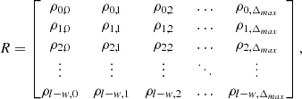
The sliding-window process provides us windowed data A and B, for which we calculate the Spearman’s rank cc, ρi, j, within two windows Ai and Bj for all possible combinations of i and j, and record all ρi, j in a matrix R. Details can be found in the Appendix.
This matrix R thus contains the values of the Spearman’s rank cc for all possible combinations of window locations (defined by i and j). In the visualization, ρi, j corresponds to a pixel located at (x, τ), where x is the timestamp of the center of the window (we are using time series as an example, data sets are not necessarily distributed in time space). Thus, we have:
 (3)
(3)
Cross-correlations without any time lag are located at τ = 0. An example of this procedure is shown in Fig. 1. Panel a in Fig. 1 shows two time series, time series 1 in blue, and time series 2 in orange. The two series were analyzed by SWCC with different window sizes in panels b–e. In this and following tests, x and y in the artificial time series are dimensionless. The x-axis is x from Eq. (3) and the y-axis (for panels b–e) is τ from Eq. (2).
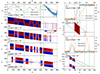 |
Fig. 1. The SWCC map for different sets of artificial time series. All maps share the same color bar shown in panel c. The black line below “window size” represents the size of the window. (a) First set of artificial time series. (b) The SWCC map with a relatively small window size of 10. (c) The SWCC map with a window size of 30. (d) The SWCC map with a window size of 90. (e) The SWCC map with a relatively large window size of 150. (f) Second set of artificial time series. Black vertical dashed lines mark the start and end time of the rising phase of time series 3, while green vertical dashed lines mark that of time series 4. (g) The SWCC map with a window size of 20. Slanted green dashed lines mark the lower and upper boundary of the parallelogram. (h) Third set of artificial time series. (i) The SWCC map with a window size of 20. Dashed lines have similar functions as those in panels g and h. |
The time series 1 is designed to be multi-structured. We marked six different regions with Roman numerals and their boundaries are indicated by vertical green dashed lines. Region I contains a simple sinusoidal signal with one peak. Region II is a small-scale (length 50) monotonically decreasing and then monotonically increasing structure. Region III is a monotonically decreasing structure followed by a sinusoidal signal of gradually increasing frequency (region IV). In the last third of this time series 1, we added a data gap (length 50, region V) and then a sinusoidal signal with increasing noise level (region VI). The time series 2 is a simple sinusoidal signal that first increases monotonically and then decreases monotonically.
The matrix R is color coded as shown in panels b–e with the color bar given in panel c; then, ρ with an absolute value lower than a certain threshold is plotted as a white pixel (background color) in our visualization. That is considered as the minimum relevant cc, ρmin, in this work, ρmin = 0.5. In all the colored maps in Fig. 1, patterns (approximate parallelograms) with distinct colors (red or blue) can be seen as well as the boundaries shown as white regions (low or no correlation). The black dashed line marks where τ = 0, we refer to this line of unshifted correlation as “baseline”; Δmax is set to be the default value here (l − w). The width of the blank space at the left and right edge of the SWCC maps correspond to half of the chosen window size. This is caused by the coordinate transformation effect mentioned in Eq. (3).
Along the baseline in panel b, time series 1 has a local maximum around x = 120, between x = 0 and x = 120, time series 1 and 2 are correlated; hence, we have a positive cc (shown in red). After the maximum we have a negative cc (shown in blue). Along a vertical line (e.g., x = 100), a windowed time series 1 is compared to a windowed time series 2 with a certain τ. When τ increases, the window on time series 2 moves to the future and the corresponding windowed data changes from monotonically increasing to first monotonically increasing and then to monotonically decreasing. Given that the windowed time series 1 is monotonically increasing, when τ increases, ρ transitions from a positive value to a negative value (red-white-blue), corresponding to the change of monotonicity in the windowed time series 2. In all SWCC maps, along a line with a slope of –1 (e.g., τ = −x + 100), the window is moving on time series 1 while the window on time series 2 has a fixed location. Similar to a vertical line, along this τ = −x + 100, the sign of ρ also changes based on the monotonicity of windowed time series 1.
Simply put, along the vertical direction and a slope of –1 direction, the sliding window passes through the different structures in time series 1 and 2, respectively. The transition between positive and negative values of cc indicates the boundary positions of those structures in the time series. The intersection of boundaries in both directions forms approximate parallelograms that mark interesting regions where windowed data from two series have a high cc.
With a relatively small window size (see Fig. 1b), SWCC successfully identified the boundaries of regions III, IV, V, and VI. The boundary between regions I and II can not be resolved by SWCC because the Spearman’s cc between time series 1 and 2 remains to be positive there. Both time series are monotonically decreasing across this boundary. The inner structures in region IV are also identified. As expected, the data gap (V) shows up as an uncorrelated region, that is, in white. The noise in region VI varies on a timescale that is longer than the window size, the value of ρ varies randomly and it is unable to detect any structures there.
Panel c shows results for an intermediate window size (which is on the order of the structures contained in the two time series). Small structures are not masked and noise does not unduly affect the results, although structure boundaries are now more blurred in the noisy region. The change from monotonic increase to decrease in time series 2 can still be seen regardless of the noise in time series 1 (on the right of Fig. 1c, upper part and lower part have distinct colors).
Panels d and e show the effect of further increasing window size. As it gets larger than the interior structures, it averages over the changes and the high cc vanishes and information about small structures is lost. That shows up as wide white bands in panels d and e. A larger window, however, also smooths out noisy time series, we can see the complete corresponding red (and blue) parallelogram in panels d and e.
Panels f and g further explain the correspondence between the boundaries of the parallelograms in the SWCC map and the features of the associated time series. Figure 1f shows artificial time series 3 and 4, each of them contains a monotonically increasing sequence with different lengths. They are connected at both ends with random noise to ensure the total length of the two sequences are the same. Black vertical dashed lines mark the start and end time of the rising phase of time series 3, while green vertical dashed lines mark that of time series 4. For the parallelogram shown in panel g, ρ is seen as red (ρ > 0.5) where the two windowed data are positively correlated but vanishes where they are not. The boundaries of the parallelogram correspond to the boundaries of the structures in the time series.
Panels h and i demonstrate SWCC’s ability to probe recurrent structures. The upper parallelograms (around x = 75, τ = 150) are almost the same as the lower ones (around x = 75, τ = 0), indicating a high degree of similarity between the windowed time series 6 around x = 75 and that at a time lag of 150 units. Although such recurrent structures in the map do not necessarily have physical meanings, SWCC is a convenient way to locate those potential time periods of interest.
To summarize, the SWCC map is essentially a visualization of a two-dimensional (2D) cross-correlation function, where one dimension represents the relative position between the two windows (τ), while the other dimension corresponds to the absolute position of the window. Each vertical profile of the map represents a one-dimensional cross-correlation function with respect to τ (Weisstein 2006; Bracewell & Kahn 1966). Figure 1 shows that with a proper window size, SWCC can pick out periods in which two time series are highly correlated and provide information related to time lags and recurrent structures.
2.3. Sliding-window mutual information method (SWMI)
The SWMI method shares the sliding-window concept with SWCC, but here we calculate the mutual information instead of the Spearman’s rank correlation. The mutual information I(𝒳, 𝒴) of two jointly discrete random variables α and β is defined as1:
 (4)
(4)
Here, 𝒳 and 𝒴 represent the set of possible values for α and β, respectively; P(α, β) denotes the joint probability mass function of α and β, while P(α) and P(β) are the marginal probability mass functions of α and β, respectively.
Normalized mutual information (IN) is simply a normalized version of MI that provides a value between 0 (no mutual information) and 1 (perfect match or knowledge), indicating the normalized amount of shared information (Pedregosa et al. 2011). In this work, mutual information is normalized by the mean value of the entropy H of 𝒳 and 𝒴. We then have:
 (5)
(5)
The normalized mutual information IN is defined as:
 (6)
(6)
Solar wind measurements need to be discretized before calculating the MI. While there are different discretization techniques, in this work we use the equal-width binning method to discretize each windowed data Ai independently by dividing the variables into a fixed number of equally sized bins and then measurements are discretized into a sequence of indices representing the bins in which each data point resides. This number, Nbins, is a problem-dependent parameter, it should be chosen based on the specific data distribution of the problem. In our study, it is determined on the basis of the Freedman–Diaconis rule (Freedman & Diaconis 1981):
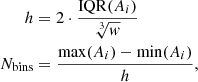 (7)
(7)
where IQR is the interquartile range obtained by calculating the difference between the third quartile (Q3) and the first quartile (Q1) of a data set. We chose this rule since it does not require an assumption of normality of the distribution. In this work, we always use Eq. (7) to decide the unique Nbins for each windowed data (Ai or Bj).
To illustrate the SWMI, we also apply it to artificial data sets y7 and y8 shown in Fig. 2a. The unshaded parts of y7 and y8 are obtained independently by randomly selecting values from a uniform distribution:

 |
Fig. 2. Two artificial series and related SWMI map. (a) The artificial time series, all values are integers. Green regions are two periods where two series have a unique mapping relationship (see Eq. (8)). Red line segments mark three positions where the distributions of windowed data are shown in following histograms. (b) Histogram of two windowed series marked by the first red line segment. (c) Histogram of two windowed series marked by the second red line segment. (d) Histogram of two windowed series marked by the third red line segment. (e) The SWMI map with a window size of 50, which is also graphically shown below the text. Green dashed lines are boundaries of the green regions in panel a. In panels b–d, the bin size is chosen according to Eq. (7). |
where k is a random integer between 0 and 20. The data in the shaded parts of y7 are randomly selected from another uniform distribution:

while the shaded parts of y8 show data that are a multi-valued function of y7:
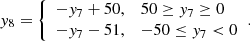 (8)
(8)
Within the shaded areas, the distribution of y7 then provides all information needed to determine the distribution of y8, so the normalized mutual information IN is 1 (when τ = 0).
Panels b–d further demonstrate the detailed distribution of three selected pairs of windowed data (τ = 0) indicated by red line segments at the bottom of panel a. Panel b shows that windowed data are randomly distributed while panel d shows the relationship between y7 and y8, while panel c is a mixture of both. Here, the histograms only show the data distributions (with Nbins determined by Eq. (7)), they are not part of the calculation of MI in this test because y7 and y8 are already of integer type.
Panel e shows the related SWMI map where IN are color coded using a different color map than for SWCC. Color maps for SWCC and SWMI are used consistently in this paper (as in Fig. 1 for SWCC and Fig. 2 for SWMI). The artificial data sets shown in panel a look totally random but the two shaded regions are clearly identified by the SWMI and are seen as red and purple patterns around the baseline in Fig. 2e. The maximum value of IN only occurs at the baseline (but is partially covered by the black dashed line in the figure, making it hard to see) because time lags break the perfect bijective relationship between y7 and y8. With a certain time lag (shown along the y-axis), we can calculate IN between windowed data in the first and second shaded region. It can be seen that related IN are high (red/purple patterns away from the baseline in Fig. 2e), which indicates the similarity between data in the two shaded areas. This is best seen by considering the start and end “times” of the shaded regions, x = 150(450) and x = 300(600), shown as vertical dashed green lines in panel e.
2.4. Window size selection
In Sect. 2.2, we show that the window size w is a crucial free parameter that affects the final ρ or IN. With sufficient prior information, that is, knowing the size of the target structures, m (timescale), we can manually choose a window size, w ≃ m, and adjust it appropriately for the specific situation. Here, we introduce a “window-island sizing” (WIS) technique to guide the choice of the window size when m is either unknown or highly variable.
In the WIS, “window” refers to the window size and the “island” size is its dependent variable, calculated from the corresponding SWCC map. An island is defined as a region in the SWCC matrix R for which |ρ|≥ϵ, where ϵ is the island eligibility threshold. Data points with ρ < ϵ are not considered to be informative. The island eligibility threshold and the minimum relevant cc should always be the same, we only name them differently to emphasize the roles they play.
We further define relative island size, η, as the ratio between island size and total size of the map,
![Mathematical equation: $$ \begin{aligned} \eta =(\sum [\rho \ge \epsilon ])/((\Delta _{\rm max}+1)\cdot (l-w+1)), \end{aligned} $$](/articles/aa/full_html/2024/04/aa48703-23/aa48703-23-eq11.gif) (9)
(9)
where the relative island size η is shown as a function of w.
Panels a and b in Fig. 3 demonstrate these kinds of curves, using data for two time periods, which are shown in more detail in Figs. 4 and 5. In panel a, we applied three different ϵ values that influence η but barely affect the overall trend of the curve. The local minimum of η of three different curves share a similar corresponding w. In this work, ϵ is set to be the same as the ρmin value mentioned in Sect. 2.2.
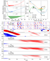 |
Fig. 3. Relative island size curves to guide the window size selection and an example of the SWCC maps of the same period but under different window sizes or time resolutions. The horizontal boundary of the shaded area (horizontal line) for each curve is defined as the minimum value of η plus 1% (or maximum minus 1%). (a) Relative island size curves with different thresholds for data used in Fig. 4, Δmax = 30 days. The black dashed line marks the window size we manually choose for the analysis in Sect. 4.1, which is 48 h. (b) Relative island size curves for data with different time resolution applied in Fig. 5. ϵ = 0.5, Δmax = 12 h. The black dashed line marks w = 25 h. The black crosses mark two local minima and one local maximum, triangles mark where w = 25 h. (c) The SWCC map for partial data (64-s resolution) applied in Fig. 5, the window size is 0.36 h, corresponding to the left cross in panel b. (d) The SWCC map for the same data applied in panel c, the window size is 9.16 h, corresponding to the middle cross in panel b. (e) The SWCC map for the same data applied in panel c, the window size is 24.99 h, corresponding to the right cross in panel b. (f) Same window size as panel e but with 4-min data. (g) Same as panel e, but with 12-min data. |
For (too) small window sizes, noise causes random short-term coincidences and/or correlations, leading to more islands (larger η). When the window size is too large (when w approaches l and τ ≃ 0), however, ρ will converge to the cc of the data as a whole. If two series have a relatively large global cc, then at both ends of the η(w) curve, we have high η. A window size that is neither too small nor too large avoids both the noise and the overall effects and thus identifies the structures worth investigating. If not many structures (islands) are found, we have low η, while high η represents a larger amount of structures, thus at least one local minimum is expected. This local minimum represents a compromise between window sizes which are too small and thus dominated by noise and window sizes which are too large and wash out all fine structure in the time series. We can see local minima in those three curves in panel a marked by horizontal black lines.
In this work, we set the minimum η plus 1%, as indicated by the height of the horizontal dashed lines in Fig. 3a as the basis for selecting the window size. This added value (we refer to this as island size margin δ) of 1% (a subjective choice) is introduced only to provide a reference range for w because a single optimal window size cannot be expected to exist. Those ranges for w used in this work are shown as shaded areas in panels a and b.
The local maximum for the intermediate window sizes represents a window size that identifies many well defined structures (islands) in the time series and represents the typical size of these structures. Therefore, if such a local maximum is available, the corresponding window size is best suited for a first look at the SWCC and SWMI maps. A local maximum also naturally brings multiple local minima, leading to different w choices. The η(w) curve for 64-s resolution data (the green one) in panel b has two local minima and one local maximum (all marked by black crosses). The first local minimum and the local maximum indicate two w choices that can not be clearly inferred from the other two curves. The second local minimum has a similar recommended window size range as the other two time resolutions do.
We further compared the related SWCC maps for three window sizes (0.36, 9.16, and 24.99 h) in panels c–e. In panel c, many small structures (tiny blue parallelograms) are identified along the baseline, which indicate an anti-correlation between solar wind density and magnetic field strength. These structures are not visible with larger window sizes and cannot be identified at higher resolution due to the limited number of data points. In panel d, two bigger positive correlation structures are found while only one is identified in panel e. This shows that different structures with different sizes are contained together in the time series, highlighting the importance of timescales in correlation analyses. Panels e–g show the SWCC maps for the same window size (25 h) but using data with different time resolution. Panels e (64-s data) and f (4-min data) are almost the same, while the structure in panel g is smaller compared to other two panels.
Again, if prior knowledge on the size of the structures of interest is available, it is preferable to bypass the WIS and adjust the window size for the size of the structures that is the subject of investigation. Nevertheless, the WIS technique can also be regarded as a tool to confirm the size of typical structures in the two time series. The WIS technique only offers a reference range for window size in cases when the size of the target structure is unknown. The related η(w) curve is a good guide for the window size selection, which also provides information about timescales that are worth investigating.
Data sets with high cc tend to have high mutual information, but not necessarily vice versa. Spearman’s rank cc takes into account both the values of data points and their order in a data set. In contrast, MI focuses on the statistical dependence between variables within specific windows, disregarding the order of data points.
Thus, a combination of Spearman’s rank cc and MI allows to understand whether a relationship is monotonic or non-monotonic (and linear or non-linear if a Pearson cc has been applied).
2.5. User guide
In the following we give a step-by-step procedure that can be followed by potential users. We assume that two data products have been chosen and the respective data are already available. (1) Choose the window size: if the timescale of structures-of-interest is already known a priori, the window size, w, can be selected accordingly. If the timescale is completely unknown or timescale itself is the research object, then using the WIS technique (see Sect. 2.4) would be reasonable. (2) Select the quantitative description of correlation one wants to analyze: such as the Pearson cc, Spearman’s rank cc, and mutual information, based on the specific needs of the study. Mutual information also requires sufficient data points within one window (over 102 is recommended). (3) Obtain visual products: the SWCC/ SWMI maps with a certain color map defined based on the needs of the study. (4) Interpret the resulting SWCC or SWMI maps: for SWCC maps with a smooth color map, the approximate parallelograms in the visual outputs represent the underlying structures. A pattern deviating from a parallelogram can indicate that the selected window size is not suitable (displayed as “overflow” for the parallelogram shape or “adherence” of adjacent patterns, suggesting that the window size may be too large). Broad band-like patterns parallel to the baseline indicate overly large window sizes. Narrow band-like patterns often signal poor data quality or that the selected window size is too small and noise dominates the map. The specific physical meaning represented by the ultimately obtained parallelograms requires a detailed analysis of the specific situation. For SWMI maps with a discretized color map, well-shaped parallelograms generally are not expected. One should focus on patterns with high IN especially inside known parallelograms in SWCC maps. (5) A combination of different quantitative descriptions is recommended: combining SWCC and SWMI maps could give indications of monotonic (or linear) and non-monotonic (or non-linear) relations between the two input variables. A combination of Pearson cc and Spearman’s rank cc (two SWCC maps) provides information about how much monotonic relationship is linear.
3. Data
In the following, we discuss our application of our methods to solar wind data, using the solar wind density, magnetic field strength, and velocity measured at 1 AU by the Advanced Composition Explorer (ACE, Stone et al. 1998) in 2007. We used the 64-s, 4-min, and 12-min averaged magnetic field data from the Magnetometer (MAG, Smith et al. 1998), along with the 64-s and 4-min averaged solar wind plasma data from the Solar Wind Electron Proton Alpha Monitor (SWEPAM, McComas et al. 1998) and 12-min solar wind plasma data from the Solar Wind Ion Composition Spectrometer (SWICS, Gloeckler et al. 1998). These data are provided by the ACE Science Center2.
4. SWCC and SWMI for solar wind parameters
In this section, we describe the application of our methods to two months of solar wind proton density and total magnetic field strength (B) because of the known time delayed relationship in stream interaction regions (SIRs). The solar wind density peaks are typically observed at or just before the onset of speed gradients, while the magnetic field peaks occur later, within the solar wind speed gradient region (Lindsay et al. 1995; Richardson 2018). A second peak in the solar wind density then indicates the region of compressed fast solar wind.
4.1. Two months of solar wind
We use data from February to March 2007 (day of the year, DOY, 32–90), over which there were no recorded ICMEs (Cane & Richardson 2003; Richardson & Cane 2010). During these two months, the overall Spearman’s rank cc (under the assumption of no time lag) of solar wind proton density and total magnetic field strength was: 0.39 for 12-min resolution data, 0.55 for 4-min resolution data, and 0.55 for 64-s resolution data. The overall normalized mutual information (Nbins chosen based on Eq. (7)) was 0.116 for 12-min resolution data, 0.138 for 4-min resolution data, and 0.111 for 64-s resolution data. We chose 48 h as the window size in this section because our target structures are SIRs and this window size is representative of the size of SIRs in this two-month period.
In Fig. 4, panel a shows B in black and density in blue. Time periods during which SWEPAM data were missing were filled in with data from SWICS (orange). Panel b shows solar wind speed in green. Comparison of panels a and b shows several SIRs in which density and B increase due to the compression caused by the fast wind running into the slow wind. The shaded region I is discussed in detail later in this work.
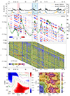 |
Fig. 4. In situ measurements related SWCC and SWMI map of two months of solar wind. (a) Solar wind density and magnetic field strength measurements. Blue shaded region marks the selected period for further study in Sect. 4.2, pink region marks the zoomed in area. (b) The SWCC map based on 12-min resolution data and solar wind velocity. (c) The SWMI map based on 12-min resolution data. (d) Zoom on panel b with extra contours. (e) Zoom on panel c, regions with relatively high IN are marked. |
Panel b is the SWCC map (w = 48 h, Δmax = 30 days) based on 12-min data shown in panel a. We can clearly identify regions of positive (red, see, e.g., the region indicated by the black arrow) and negative (blue) correlation between solar wind density and magnetic field strength along the baseline (τ = 0). Positive correlations are more frequent than negative ones because compression and rarefaction affect both density and the magnetic field strength. This illustrates that a long-term correlation is not necessarily representative for the dynamics on shorter timescales. The y-axis has been extended to ±30 days and we expect similar co-rotating interaction regions to show up as red parallelograms at ±27 days. We can find red parallelograms at τ = ±27 and their corresponding red ones at τ = 0. Apart from this expected signature of solar rotation, we identified potential shorter term recurrent structures based on this map. For example, we first locate the red parallelogram at the baseline around DOY 60 (indicated by the black arrow in panel b), then we have two other red parallelograms above it, corresponding to two other SIRs following region I.
For the SWMI map (panel c), most regions with relatively high normalized mutual information, IN, appear at locations with high cc in the SWCC map (panel b). We further zoom in the same area (marked by black dotted-dashed lines) in the two maps respectively in panels d and e. In panel d, we added extra contours for lower cc, thus, we can see how the islands change if ϵ is set to be 0.3. Three regions, R1, R2, and R3, with high IN are pointed out and tagged in panel e. From the combination of both panels, we can see that R3 in panel e corresponds to the red pattern (high cc) in panel d. However, R1 and R2 belong to regions with low cc values, indicating a potential non-linear relationship that is not monotonic either. R1, R2, and R3 represent the same period of rising density in the compressed slow solar wind region, but different periods of magnetic field; also, the density there displays a high MI towards local and former (1.5 and 3 h) magnetic field strength which also belong to slow solar wind around DOY 42. High MI indicates good mapping relationships between density and B, which is in the form of monotonic in R3 but non-monotonic in R1 and R2. Establishing a certain relationship among data within R1, R2 and R3 is more likely to achieve more reliable results than other data with low mutual information. In this case, magnetic field strength in the uncompressed slow solar wind can be used to predict density in the compressed slow solar wind a few hours later. Unfortunately, high time-resolution SWEPAM data are not available around this zoomed in area.
The SWCC map clearly identifies and displays the monotonic relationships between two series with temporal lags taken into consideration. The SWMI map verifies those monotonic relationships and also reveals non-monotonic relationships. Combining these two parts, our tool then combines cc and MI together to deepen the understanding of relationships between two series. For example, regions with high MI (from SWMI maps) can be marked as areas that have the potential to establish a reasonable relationship between two series, SWCC maps tell us whether the relationship is monotonic. In other words, our methods are suitable for playing as a filter and pre-selection tool that pick out highly related data sets.
4.2. Selected time period
From the two months, we picked one time period with complete SWEPAM data coverage and that includes a SIR and the trailing high speed stream. This period is marked as period I and is shaded in blue in Fig. 4a, its boundaries are marked by dotted-dashed lines there. We chose the window size to be 9.16 h according to the relative island size curves (the local maximum labeled “go to (d)”) in Fig. 3b. We only show SWCC and SWMI maps based on 64-s data because the SWCC maps are similar for data at the other two time resolutions (see Fig. 3; panels f–h) and SWMI requires high time resolution to obtain sufficient statistics.
In Fig. 5, we show the data and derived information for period i, which covers a high-speed stream and a preceding SIR. Panel a is a zoomed-in version of Fig. 4b together with solar wind velocity measurements. We can see a rather large red pattern (positive correlation) with clear upper and lower boundaries (around DOY 59–60.5). However, in the detailed SWCC map (panel b), several smaller structures are identified around the baseline, some of them are marked by lowercase Roman numerals that will be discussed shortly. Panel c shows the MI for the same time period and panel d shows IMF and solar wind density. We used these quantities to compute the cc and MI.
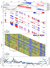 |
Fig. 5. SWCC and SWMI map of the selected time period I in Fig. 4a. Window sizes, number of data points in each window, and the visible window scales are marked below the serial number of each sub-plot. (a) Zoom on Fig. 4b. (b) The SWCC map based on 64-s resolution data. Black arrows mark six structures with high cc. Green dotted-dashed lines mark the region which is analyzed in Fig. 3. (c) The SWMI map based on 64-s resolution data. Black rectangles mark two regions analyzed in Fig. 6. (d) 64-s resolution solar wind proton density and magnetic field strength measurements. |
In the following, we discuss the features indicated by roman numerals in panel b. Structure (i) corresponds to the compressed slow solar wind where the solar wind density and magnetic field strength both increase. The following structure (ii) corresponds to the compressed fast solar wind where the two solar wind parameters both decreased, but the related cc is just above 0.5, making the red pattern pale. The time lag between density peak and magnetic field strength peak indicated by structures (i) and (ii) is short in this case. Structure (iii) compares density in the compressed fast solar wind (measured after DOY 58.5) with B in the preceding compressed slow solar wind (measured after DOY 58), resulting in the anti-correlation that can be seen there. Structures (i) and (iii) also have relatively high IN on the SWMI map in panel c, but structure (ii) does not show high IN. This area encompassing structures (i) to (iii) is highlighted by the green dash-dotted rectangle and is discussed further in Fig. 6. Structures (iv) and (v) represent short-term positive correlations within the high speed stream, whose locations are close to the beginning and end of the stream. Structures (i), (ii), (iv), and (v) have relatively high IN on the SWMI map in panel c. Right before structure (v), there is a short period (∼5 h) of solar wind where cc and MI are both low, which shows the independence between density and B, indicating potential interfaces in the high speed stream. Structure (vi) occurs after the rarefaction region where the density experiences a small rise, but the SMMI map in this area does not correspond to the SWCC map very well, details can be found in Fig. 6.
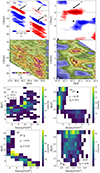 |
Fig. 6. Zoom on SWCC and SWMI maps for two rectangular areas marked in Fig. 5c, and detailed data distribution examples. Histograms shown here use Nbins determined by Eq. (7), with the calculated ρ and IN marked as well. |
Figure 6 shows zoomed-in maps for the two rectangular areas marked in Fig. 5c. The left column in Fig. 6 is for the left and also larger rectangular area. Panel a is a zoomed-in SWCC map, panel b is a zoomed in SWMI map, where we mark two spots with a black cross and a star, respectively, inside structures (ii) and (iii), where we have high ρ but low IN (cross) and both high ρ and IN (star). Panels c and d demonstrate the detailed data distributions at those two markers’ locations as well as the discretization based on Eq. (7). We can see that the highest IN appears in structure (iii), indicating the potential capability to predict compressed fast solar wind properties based on compressed slow solar wind ahead. The different distributions of B versus n in panels c and d result in clear differences in cc and MI. The cc of 0.51 in panel c just barely exceeds our (subjective) threshold of 0.5 which is probably also reflected in the weak MI. On the other hand, the strong anti-correlation in panel d results in a high MI.
The right-hand column of Fig. 6 corresponds to the other rectangular area highlighted in Fig. 5. We also mark two spots by a black circle and a triangle where we have low ρ but high IN (circle) and both low ρ and IN (triangle). Panel g shows how SWMI captures non-monotonic relationships between two parameters that can not be recognized by cross-correlation. In this panel, density and B are positively correlated when the density is below 6 cm−3 but the overall ρ is –0.39. The negative cc is driven by the overall 2D distribution which is determined by two patches, one at high B but low density, with the other by low B and high density. The MI however, recognizes that there is a (complicated) relationship between B and density. Panel h shows how the data distributed when ρ and IN are both low, which is a case where we may consider density and B to be independent.
The detailed analysis of this selected time period demonstrates the potential of our methods especially combined with high time resolution data. In this example, short-term positive correlation structures are found when τ ≃ 0 and two of them are related to compressed regions of SIRs. The zoomed in maps and detailed data distributions illustrate the main advantage of combining cc and MI together, that is verifying monotonic relationships and digging out non-monotonic relationships. A data distribution like panel d can be found only based on the SWCC map, and monotonic relationship is generally enough in some cases. However a data distribution such as that shown in panel g, requires a combination of cc and MI stands as a promising means for extracting more complex relationships from such a distribution. That is why our methods can serve as a data filter, while any interesting data distributions that come about as a result can be picked up for further study.
5. Discussion
Our approach combines cross-correlation and mutual information analysis, both of which are well-established methods for describing relationships between variables. By incorporating a sliding window technique, timescales (through w), and temporal or spatial lag effects (through τ) are taken into consideration.
WIS helps to indicate the scales of the underlying structure, thus providing reasonable window sizes for further study. For a certain window size, SWCC can conveniently characterize the locations of underlying structures that possess monotonic relationships. Of course, it is possible to easily switch the Spearman’s rank correlation to the Pearson correlation in order to search for pure linear relationships and/or to combine both the Pearson’s and Spearman’s ccs to discriminate between linear and monotonic relationships. Then, SWMI can be used to further verify such monotonic relationships, while non-monotonic relationships can be identified by comparing two related maps. Cross-correlations compare times series that are not expected to repeat in most cases, while MI compares (repeatable) distributions that can help to identify solar wind with similar properties (from similar source regions or due to similar transport effects). A combination of SWCC and SWMI can be seen as a data filter and can also be incorporated into the preprocessing procedures of machine learning. For example, in the field of space weather prediction, we aim to establish reasonable relationships between different parameters related to physical conditions at the Sun, in the solar wind, and in near-Earth space. Thus, we need to find out which two parameters are independent and relevant and also “when” they are applicable. High mutual information means there are more information for digging, and its application in the field of space weather prediction has precedent (Materassi et al. 2011; Alberti et al. 2017).
Higher time resolution reduces the step size of the sliding-window, in the case of which the boundaries of underlying structures can be identified more precisely and the identification of smaller structures becomes possible. Higher time resolution also provides more data points inside a fixed-length window, making MI calculation more reliable. The high time resolution data from Solar Orbiter (Müller et al. 2020; Owen et al. 2020) and Parker Solar Probe (Bale et al. 2019) are expected to enhance the practical applicability of our approach.
Between the density and magnetic field strength, we identified long-term positive correlations (>12 h, see Fig. 3e), medium-term positive correlations (∼7 h, see Fig. 3d), and short-term negative correlations (∼10 min, see Fig. 3c) which exist together in the compressed solar wind sample with τ ≃ 0. Such long-term positive correlations have been previously observed, for instance, Xia & Marsch (2003) used remote-sensing data to estimate the proton density using electron density, finding that the mass flux of the nascent fast solar wind may be directly associated with the net flux density of the magnetic field in the coronal hole. Short-term negative correlations could be more interesting and may be related to pressure-balanced structures (Burlaga & Ogilvie 1970), where statistically the proton density and magnetic field strength tend to be anti-correlated (Marsch & Tu 1993; Tu & Marsch 1994; Yao et al. 2013). The SWCC is useful to identify such structures. We present two more examples in the Appendix to show the applications of SWCC (see Appendix B).
Figures 4 and 6 show the benefits of combining cross-correlation and mutual information to identify non-monotonic relationships between density and magnetic field strength, which merit future investigation.
6. Conclusions
In this work, we apply the concepts of cross-correlation and mutual information to the analysis of solar wind data and exemplify it using solar wind density and magnetic field measurements from ACE. Certainly, other combinations of parameters, especially the kinetic properties of the solar wind (3D velocity and 3D temperature) and composition, would also merit similar investigations, but they are beyond the scope of the present study.
By integrating the sliding-window cross-correlation and sliding-window mutual information, we can investigate monotonic+linear and non-monotonic+non-linear relationships between two data sets and identify the underlying structures. Those structures can then be visually represented as colored patterns on a map; if patterns are well-shaped parallelograms, a temporal or spatial lag can be estimated reliably. These kinds of visual products from our tool provide an innovative and intuitive point of view towards the data compared to traditional numerical methods, which have been established for around one century. Timescales are shown as the size and shape of the patterns and underlying temporal lags are indicated by their positions relative to the baseline. Our tools could also be useful in analyzing multi-wavelength photometric and spectroscopic time series.
Correlations with different timescales can coexist, thus, global correlations may not always capture local properties accurately. This can be overcome by tailoring the method to the specific problem at hand by adjusting the size of the window and combining results from SWCC, SWMI, and WIS. Such tailoring can reveal intricate variations and dependencies, as we show in Figs. 3 and 5.
Our approach combines monotonic (or linear) and non-monotonic (or non-linear) relationships, timescale analysis, and intrinsic lag effects. It may serve as a powerful tool to identify previously undiscovered relationships between data sets.
In this work, we use the natural logarithm, the unit of mutual information is then given as “nat”. If the log base 2 is used, the unit of mutual information is shannon, also known as bit, which is more common in computer science and machine learning.
http://www.srl.caltech.edu/ACE/ASC/level2 (retrieved August, 1, 2023).
http://wdc.kugi.kyoto-u.ac.jp/wdc/Sec3.html(Imajo et al. 2022). (Retrieved December, 19, 2023).
Acknowledgments
This work is supported by China Scholarship Council (CSC) under the file number: 202106400008. Verena Heidrich-Meisner is supported by German Space Agency (DLR) grant number 50OC2104.
References
- Adhikari, B., Dahal, S., Sapkota, N., et al. 2018, Earth Space Sci., 5, 440 [NASA ADS] [CrossRef] [Google Scholar]
- Alberti, T., Consolini, G., Lepreti, F., et al. 2017, J. Geophys. Res. Space Phys., 122, 4266 [NASA ADS] [CrossRef] [Google Scholar]
- Asbridge, J. R., Bame, S. J., Feldman, W. C., & Montgomery, M. D. 1976, J. Geophys. Res., 81, 2719 [NASA ADS] [CrossRef] [Google Scholar]
- Bale, S. D., Badman, S. T., Bonnell, J. W., et al. 2019, Nature, 576, 237 [NASA ADS] [CrossRef] [Google Scholar]
- Barrow, C. H. 1978, Planet. Space Sci., 26, 1193 [NASA ADS] [CrossRef] [Google Scholar]
- Benesty, J., Chen, J., Huang, Y., & Cohen, I. 2009, Pearson Correlation Coefficient (Berlin, Heidelberg: Springer), 1 [Google Scholar]
- Berger, L. 2008, Ph.D. Thesis, Kiel University, Germany [Google Scholar]
- Bracewell, R. 1965, Pentagram Notation for Cross Correlation. The Fourier Transform and its Applications (New York: McGraw-Hill), 46, 243 [Google Scholar]
- Bracewell, R., & Kahn, P. B. 1966, Am. J. Phys., 34, 46 [Google Scholar]
- Burlaga, L. F., & Ogilvie, K. W. 1970, Sol. Phys., 15, 61 [NASA ADS] [CrossRef] [Google Scholar]
- Cameron, T., Jackel, B., & Oliveira, D. 2019, J. Geophys. Res. Space Phys., 124, 1582 [NASA ADS] [CrossRef] [Google Scholar]
- Cane, H. V., & Richardson, I. G. 2003, J. Geophys. Res. Space Phys., 108, 1156 [NASA ADS] [CrossRef] [Google Scholar]
- Cane, H. V., Richardson, I. G., & St. Cyr, O. C. 2000, Geophys. Res. Lett., 27, 3591 [NASA ADS] [CrossRef] [Google Scholar]
- D’Amicis, R., De Marco, R., Bruno, R., & Perrone, D. 2019, A&A, 632, A92 [NASA ADS] [CrossRef] [EDP Sciences] [Google Scholar]
- De Winter, J. C., Gosling, S. D., & Potter, J. 2016, Psychol. Methods, 21, 273 [CrossRef] [Google Scholar]
- Duncan, T. E. 1970, SIAM J. Appl. Math., 19, 215 [CrossRef] [Google Scholar]
- Freedman, D., & Diaconis, P. 1981, Zeitschrift für Wahrscheinlichkeitstheorie und verwandte Gebiete, 57, 453 [CrossRef] [Google Scholar]
- Fung, S. F., & Tan, L. C. 1998, Geophys. Res. Lett., 25, 2361 [NASA ADS] [CrossRef] [Google Scholar]
- Geiss, J., Gloeckler, G., & von Steiger, R. 1995a, Space Sci. Rev., 72, 49 [NASA ADS] [CrossRef] [Google Scholar]
- Geiss, J., Gloeckler, G., von Steiger, R., et al. 1995b, Science, 268, 1033 [Google Scholar]
- Georgieva, K., Kirov, B., Tonev, P., Guineva, V., & Atanasov, D. 2007, Adv. Space Res., 40, 1152 [NASA ADS] [CrossRef] [Google Scholar]
- Gloeckler, G., Cain, J., Ipavich, F. M., et al. 1998, Space Sci. Rev., 86, 497 [NASA ADS] [CrossRef] [Google Scholar]
- Gosling, J. T., McComas, D. J., Phillips, J. L., & Bame, S. J. 1991, J. Geophys. Res., 96, 7831 [Google Scholar]
- Gu, C., Heidrich-Meisner, V., Wimmer-Schweingruber, R. F., & Yao, S. 2023a, A&A, 671, A63 [NASA ADS] [CrossRef] [EDP Sciences] [Google Scholar]
- Gu, C., Heidrich-Meisner, V., & Wimmer-Schweingruber, R. F. 2023b, in EGU General Assembly Conference Abstracts, EGU–2841 [Google Scholar]
- Imajo, S., Matsuoka, A., Toh, H., et al. 2022, Mid-latitude Geomagnetic Indices ASY and SYM (ASY/SYM Indices) (Kyoto: World Data Center for Geomagnetism) [Google Scholar]
- Iyemori, T., & Rao, D. R. K. 1996, Annales Geophysicae, 14, 608 [NASA ADS] [CrossRef] [Google Scholar]
- Kasper, J., Stevens, M., Korreck, K., et al. 2012, ApJ, 745, 162 [CrossRef] [Google Scholar]
- Kocher, M., Lepri, S. T., Landi, E., Zhao, L., Manchester, W. B. I., 2017, ApJ, 834, 147 [NASA ADS] [CrossRef] [Google Scholar]
- Kraskov, A., Stögbauer, H., & Grassberger, P. 2004, Phys. Rev. E, 69, 066138 [NASA ADS] [CrossRef] [Google Scholar]
- Lepri, S. T., Laming, J. M., Rakowski, C. E., & von Steiger, R. 2012, ApJ, 760, 105 [NASA ADS] [CrossRef] [Google Scholar]
- Li, D., & Yao, S. 2020, ApJ, 891, 79 [CrossRef] [Google Scholar]
- Lindsay, G. M., Russell, C. T., & Luhmann, J. G. 1995, J. Geophys. Res., 100, 16999 [NASA ADS] [CrossRef] [Google Scholar]
- Maksimovic, M., Bale, S. D., Berčič, L., et al. 2020, ApJS, 246, 62 [Google Scholar]
- March, T., Chapman, S. C., & Dendy, R. O. 2005, Geophys. Res. Lett., 32, L04101 [CrossRef] [Google Scholar]
- Marsch, E., & Tu, C. Y. 1993, Ann. Geophys., 11, 659 [Google Scholar]
- Marsch, E., Mühlhäuser, K.-H., Schwenn, R., et al. 1982, J. Geophys. Res. Space Phys., 87, 52 [NASA ADS] [CrossRef] [Google Scholar]
- Marsch, E., Pilipp, W. G., Thieme, K. M., & Rosenbauer, H. 1989, J. Geophys. Res., 94, 6893 [NASA ADS] [CrossRef] [Google Scholar]
- Marubashi, K. 1995, Adv. Space Res., 16, 111 [NASA ADS] [CrossRef] [Google Scholar]
- Materassi, M., Ciraolo, L., Consolini, G., & Smith, N. 2011, Adv. Space Res., 47, 877 [NASA ADS] [CrossRef] [Google Scholar]
- McComas, D. J., Bame, S. J., Barker, P., et al. 1998, Space Sci. Rev., 86, 563 [CrossRef] [Google Scholar]
- Müller, D., St. Cyr, O. C., Zouganelis, I., et al. 2020, A&A, 642, A1 [Google Scholar]
- Owen, C. J., Bruno, R., Livi, S., et al. 2020, A&A, 642, A16 [EDP Sciences] [Google Scholar]
- Pedregosa, F., Varoquaux, G., Gramfort, A., et al. 2011, J. Mach. Learn. Res., 12, 2825 [Google Scholar]
- Richardson, I. G. 2018, Liv. Rev. Sol. Phys., 15, 1 [Google Scholar]
- Richardson, I. G., & Cane, H. V. 2010, Sol. Phys., 264, 189 [NASA ADS] [CrossRef] [Google Scholar]
- Riley, P., Luhmann, J., Opitz, A., Linker, J. A., & Mikic, Z. 2010, J. Geophys. Res. Space Phys., 115, A11104 [NASA ADS] [Google Scholar]
- Russell, C. T., & McPherron, R. L. 1973, J. Geophys. Res., 78, 92 [NASA ADS] [CrossRef] [Google Scholar]
- Shannon, C. E. 1948, BSTJ, 27, 379 [Google Scholar]
- Shi, C., Velli, M., Lionello, R., et al. 2023, ApJ, 944, 82 [NASA ADS] [CrossRef] [Google Scholar]
- Simms, L. E., Engebretson, M. J., & Reeves, G. D. 2022, J. Geophys. Res. Space Phys., 127, e2021JA030021 [NASA ADS] [CrossRef] [Google Scholar]
- Smith, C. W., L’Heureux, J., Ness, N. F., et al. 1998, Space Sci. Rev., 86, 613 [Google Scholar]
- Stone, E. C., Frandsen, A. M., Mewaldt, R. A., et al. 1998, Space Sci. Rev., 86, 1 [Google Scholar]
- Tu, C. Y., & Marsch, E. 1994, J. Geophys. Res., 99, 21481 [NASA ADS] [CrossRef] [Google Scholar]
- Ventura, R., Antonucci, E., Downs, C., et al. 2023, A&A, 675, A170 [NASA ADS] [CrossRef] [EDP Sciences] [Google Scholar]
- Virtanen, P., Gommers, R., Oliphant, T. E., et al. 2020, Nat. Methods, 17, 261 [Google Scholar]
- Wanliss, J. A., & Showalter, K. M. 2006, J. Geophys. Res. Space Phys., 111, A02202 [NASA ADS] [CrossRef] [Google Scholar]
- Weisstein, E. W. 2006, Correlation Coefficient (Wolfram Research, Inc.), https://mathworld.wolfram.com/ [Google Scholar]
- Wing, S., Johnson, J. R., Turner, D. L., Ukhorskiy, A. Y., & Boyd, A. J. 2022, J. Geophys. Res. Space Phys., 127, e30246 [NASA ADS] [CrossRef] [Google Scholar]
- Xia, L., & Marsch, E. 2003, AIP Conf. Proc., 679, 319 [NASA ADS] [CrossRef] [Google Scholar]
- Yao, S., He, J. S., Tu, C. Y., Wang, L. H., & Marsch, E. 2013, ApJ, 776, 94 [NASA ADS] [CrossRef] [Google Scholar]
- Yermolaev, Y. I., Lodkina, I. G., Nikolaeva, N. S., & Yermolaev, M. Y. 2010, Cosm. Res., 48, 485 [NASA ADS] [CrossRef] [Google Scholar]
- Yoo, J.-C., & Han, T. H. 2009, CSSP, 28, 819 [Google Scholar]
- Zhang, J., Richardson, I. G., Webb, D. F., et al. 2007, J. Geophys. Res. Space Phys., 112, A10102 [NASA ADS] [Google Scholar]
- Zhao, L., Zurbuchen, T. H., & Fisk, L. A. 2009, Geophys. Res. Lett., 36, L14104 [NASA ADS] [CrossRef] [Google Scholar]
Appendix A: Mathematical backgrounds of the SWCC
We determined the Spearman’s rank correlation coefficient, ρi, j, within two windows, Ai and Bj, for all possible combinations of i and j based on the following steps:
-
Calculate the rank variables for them, denoted as RAi and RBj. The average rank for RAi and RBj are denoted as
 and
and  .
. -
Calculate the covariance denoted as CovAB, as well as the standard deviations of the ranks RAi and RBj, σA and σB:
![Mathematical equation: $$ \begin{aligned} \begin{aligned} \mathrm{Cov}_{AB}&= \frac{1}{n} \sum _{k=1}^{n} (R_{A_{i}}[k] - \bar{R}_{A_{i}})(R_{B_{j}}[k] - \bar{R}_{B_{j}}),\\ \sigma _A&= \sqrt{\frac{1}{n} \sum _{k=1}^{n} (R_{A_{i}}[k] - \bar{R}_{A_{i}})^2},\\ \sigma _B&= \sqrt{\frac{1}{n} \sum _{k=1}^{n} (R_{B_{j}}[k] - \bar{R}_{B_{j}})^2}. \end{aligned} \end{aligned} $$](/articles/aa/full_html/2024/04/aa48703-23/aa48703-23-eq14.gif) (A.1)
(A.1)where RAi[k] means the k − th element in RAi.
-
The Spearman’s rank correlation coefficient is given by:
 (A.2)
(A.2)
In the end, we have a matrix R for all calculated ρi, j as:
Appendix B: Extra application examples of the SWCC and SWMI
Here, we provide two extra examples of the application of the SWCC map. We also applied the SWMI to the second example. The first example is the application of SWCC to heavy ion signatures in the solar wind. The charge states of iron and oxygen ions would freeze in at different heights in the low corona (Geiss et al. 1995b; Lepri et al. 2012; Kocher et al. 2017), thus carrying important temperature profile information of their source region. Panel (a) in Fig. B.1 shows the averaged charge states of iron and oxygen ions calculated based on the pulse height amplitude (PHA) data from ACE/SWICS (Gloeckler et al. 1998) and a detailed and extensive description of the data analysis procedure is given in Berger’s PhD thesis (Berger 2008). We used a five-hour length window (based on prior information (Gu et al. 2023a)) and conducted a SWCC scan on ten years of the heavy ion data. Panel (b) shows one of the well-shaped structures we have found. The boundaries are clear even though the upper part of the red parallelogram is cut off. Similarly to the situation shown in Fig. 1g, a clear time lag can be seen as the baseline goes through the lower part of the parallelogram. The averaged charge state of iron drops earlier than oxygen, the estimated time lags are 4.5 hours (the starts of the fall) and 8 hours (the ends of the fall), according to the side lengths of the two grey triangles. Such nice time lagged cases have not been studied in detail while a few cases like this have been reported (Gu et al. 2023b) and they are found also based on the SWCC tool in an early development stage. A SWCC scan like this is time-saving when δmax is small (focus set around the baseline) and the visual outputs from SWCC offer very intuitive information of those interesting structures. As we were limited by the amount of data within the window here, we did not further apply the SWMI to this data set.
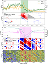 |
Fig. B.1. Two examples of the SWCC map. (a) Averaged charge states of iron and oxygen ions measured by ACE/SWICS. The time resolution is 12 minutes. (b) The SWCC map of averaged charge states of iron and oxygen ions in solar wind. w = 5 hours. Green dashed lines mark the left and right boundaries of the red parallelogram. Grey triangles are defined by the boundaries of the parallelogram and the baseline. (c) Measured z component of the solar wind magnetic field (Bz in Geocentric Solar Ecliptic coordinate system) from ACE and the symmetric disturbances for horizontal component of the geomagnetic field (SYM-H) provided by the WDC for Geomagnetism, Kyoto. The time resolution is 1 minute. w = 3.5 hours. (d) The SWCC map of Bz and SYM-H. Violet dashed lines show the left and right boundaries of the two red parallelogram that marked as structures i and ii. Grey triangles are defined by the boundaries of the parallelogram and the baseline. (e) The SWMI map of Bz and SYM-H. We mark four sub-structures of structure i and ii as structures i − 1, i − 2, ii − 1, and ii − 2. |
The second example is the application to the z component of solar wind magnetic field (Bz) and the symmetric disturbances for horizontal component of the geomagnetic field (SYM-H). Panel (c) shows Bz measured by ACE and SYM-H provided by the World Data Center (WDC) for Geomagnetism, Kyoto3. Bz has been averaged based on the original 16-sec time resolution data in order to share the same time stamps as SYM-H data. SYM-H index is considered as a high time resolution Disturbance Storm Time (Dst) index (Wanliss & Showalter 2006; Iyemori & Rao 1996) which can reveal the intensity of the globally symmetrical equatorial electrojet. Bz and Dst/SYM-H index are considered to be closely related (Russell & McPherron 1973; Gosling et al. 1991; Cane et al. 2000; Li & Yao 2020). There is about a two-hour delay in the Dst/SYM-H response (Zhang et al. 2007; Yermolaev et al. 2010), because of the traveling time of the solar wind from ACE spacecraft to the Earth. In panel (c), we can clearly see a geomagnetic storm happened around DOY 324.8 where SYM-H index had an extremely low value. Also, Bz falls from approximately 40 to -45 (from northward to southward) a few hours earlier than in the SYM-H index. We set the window size as 3.5 hours for this specific case. The SWCC map shown in (d) illustrates two well-shaped structures related to the main phase and the recovery phase of the storm. The estimated time lags related to structure (i) (main phase) are 1.75 hours (the starts of the fall) and 3 hours (the ends of the fall) according to the side lengths of the grey triangles. The estimated time lags related to structure (ii) (recovery phase) are 2.6 hours (the starts of the rise/recovery) and 4.2 hours (the ends of the rise/recovery) according to the side lengths of the grey triangles. Structure (ii) has more disturbances compared to structure (i), shown as white irregular plaques inside the parallelogram and the overflow of red color at its edges. The SWCC map intuitively shows that the main phase and recovery phase of this geomagnetic storm have different timescales and also different temporal lags between Bz and SYM-H index. We further applied the SWMI to these two data sets and the related map is shown in panel (e). Structure (i) is divided into upper and lower sub-structures with high IN, while structure (ii) is divided into left and right sub-structures with high IN. Sub-structure (i − 2) and (ii − 2) show that Bz and SYM-H index share more mutual information at the later part of both main phase and recovery phase. Sub-structure (i − 1) and (ii − 1) represent the same period of Bz (the valley position, around DOY 324.7), which has high IN with the SYM-H index 2 hours earlier and 6 hours later. Sub-structures (i − 1) and (i − 2) can hardly be seen in panel (d), indicating the potential of combining SWCC and SWMI together.
These two extra examples demonstrates the potential of our tool to be applied to a broader variety of data types. Such visual products (maps) are suitable for a vast range of data analysis fields, not limited to solar physics.
All Tables
All Figures
|
Fig. 1. The SWCC map for different sets of artificial time series. All maps share the same color bar shown in panel c. The black line below “window size” represents the size of the window. (a) First set of artificial time series. (b) The SWCC map with a relatively small window size of 10. (c) The SWCC map with a window size of 30. (d) The SWCC map with a window size of 90. (e) The SWCC map with a relatively large window size of 150. (f) Second set of artificial time series. Black vertical dashed lines mark the start and end time of the rising phase of time series 3, while green vertical dashed lines mark that of time series 4. (g) The SWCC map with a window size of 20. Slanted green dashed lines mark the lower and upper boundary of the parallelogram. (h) Third set of artificial time series. (i) The SWCC map with a window size of 20. Dashed lines have similar functions as those in panels g and h. |
| In the text | |
|
Fig. 2. Two artificial series and related SWMI map. (a) The artificial time series, all values are integers. Green regions are two periods where two series have a unique mapping relationship (see Eq. (8)). Red line segments mark three positions where the distributions of windowed data are shown in following histograms. (b) Histogram of two windowed series marked by the first red line segment. (c) Histogram of two windowed series marked by the second red line segment. (d) Histogram of two windowed series marked by the third red line segment. (e) The SWMI map with a window size of 50, which is also graphically shown below the text. Green dashed lines are boundaries of the green regions in panel a. In panels b–d, the bin size is chosen according to Eq. (7). |
| In the text | |
|
Fig. 3. Relative island size curves to guide the window size selection and an example of the SWCC maps of the same period but under different window sizes or time resolutions. The horizontal boundary of the shaded area (horizontal line) for each curve is defined as the minimum value of η plus 1% (or maximum minus 1%). (a) Relative island size curves with different thresholds for data used in Fig. 4, Δmax = 30 days. The black dashed line marks the window size we manually choose for the analysis in Sect. 4.1, which is 48 h. (b) Relative island size curves for data with different time resolution applied in Fig. 5. ϵ = 0.5, Δmax = 12 h. The black dashed line marks w = 25 h. The black crosses mark two local minima and one local maximum, triangles mark where w = 25 h. (c) The SWCC map for partial data (64-s resolution) applied in Fig. 5, the window size is 0.36 h, corresponding to the left cross in panel b. (d) The SWCC map for the same data applied in panel c, the window size is 9.16 h, corresponding to the middle cross in panel b. (e) The SWCC map for the same data applied in panel c, the window size is 24.99 h, corresponding to the right cross in panel b. (f) Same window size as panel e but with 4-min data. (g) Same as panel e, but with 12-min data. |
| In the text | |
|
Fig. 4. In situ measurements related SWCC and SWMI map of two months of solar wind. (a) Solar wind density and magnetic field strength measurements. Blue shaded region marks the selected period for further study in Sect. 4.2, pink region marks the zoomed in area. (b) The SWCC map based on 12-min resolution data and solar wind velocity. (c) The SWMI map based on 12-min resolution data. (d) Zoom on panel b with extra contours. (e) Zoom on panel c, regions with relatively high IN are marked. |
| In the text | |
|
Fig. 5. SWCC and SWMI map of the selected time period I in Fig. 4a. Window sizes, number of data points in each window, and the visible window scales are marked below the serial number of each sub-plot. (a) Zoom on Fig. 4b. (b) The SWCC map based on 64-s resolution data. Black arrows mark six structures with high cc. Green dotted-dashed lines mark the region which is analyzed in Fig. 3. (c) The SWMI map based on 64-s resolution data. Black rectangles mark two regions analyzed in Fig. 6. (d) 64-s resolution solar wind proton density and magnetic field strength measurements. |
| In the text | |
|
Fig. 6. Zoom on SWCC and SWMI maps for two rectangular areas marked in Fig. 5c, and detailed data distribution examples. Histograms shown here use Nbins determined by Eq. (7), with the calculated ρ and IN marked as well. |
| In the text | |
|
Fig. B.1. Two examples of the SWCC map. (a) Averaged charge states of iron and oxygen ions measured by ACE/SWICS. The time resolution is 12 minutes. (b) The SWCC map of averaged charge states of iron and oxygen ions in solar wind. w = 5 hours. Green dashed lines mark the left and right boundaries of the red parallelogram. Grey triangles are defined by the boundaries of the parallelogram and the baseline. (c) Measured z component of the solar wind magnetic field (Bz in Geocentric Solar Ecliptic coordinate system) from ACE and the symmetric disturbances for horizontal component of the geomagnetic field (SYM-H) provided by the WDC for Geomagnetism, Kyoto. The time resolution is 1 minute. w = 3.5 hours. (d) The SWCC map of Bz and SYM-H. Violet dashed lines show the left and right boundaries of the two red parallelogram that marked as structures i and ii. Grey triangles are defined by the boundaries of the parallelogram and the baseline. (e) The SWMI map of Bz and SYM-H. We mark four sub-structures of structure i and ii as structures i − 1, i − 2, ii − 1, and ii − 2. |
| In the text | |
Current usage metrics show cumulative count of Article Views (full-text article views including HTML views, PDF and ePub downloads, according to the available data) and Abstracts Views on Vision4Press platform.
Data correspond to usage on the plateform after 2015. The current usage metrics is available 48-96 hours after online publication and is updated daily on week days.
Initial download of the metrics may take a while.