| Issue |
A&A
Volume 692, December 2024
|
|
|---|---|---|
| Article Number | A191 | |
| Number of page(s) | 15 | |
| Section | The Sun and the Heliosphere | |
| DOI | https://doi.org/10.1051/0004-6361/202451797 | |
| Published online | 16 December 2024 | |
Short-term anticorrelations between in situ averaged charge states of Fe and O in the solar wind
Institute of Experimental and Applied Physics, Christian-Albrechts-University Kiel, Leibnizstraße 11, 24118 Kiel, Germany
⋆ Corresponding author; This email address is being protected from spambots. You need JavaScript enabled to view it.
Received:
5
August
2024
Accepted:
7
November
2024
Abstract
Context. Observations of the Fe and O charge states in the solar wind and interplanetary coronal mass ejections (ICMEs) generally exhibit a positive correlation between the average charge states of Fe and O (avQFe and avQO). Because Fe and O charge states freeze at different heights in the corona, this positive correlation indicates that conditions at different heights in the corona vary as a whole.
Aims. We identify short time periods in the solar wind that exhibit anticorrelations between the average Fe and O charge states and investigate their properties. We aim to distinguish whether these anticorrelations are due to the related solar sources or to transport effects (e.g., differential streaming). We study kinetic properties of the solar wind related to these anticorrelated structures as well as heavy ion differential streaming in order to infer a possible relationship between conditions in coronal source regions and the reported in situ measurements.
Methods. We employed a recently developed sliding-window cross-correlation method to locate anticorrelated structures in the solar wind composition measurements between 2001 and 2010 from the Advanced Composition Explorer (ACE). To account for fluctuations and measurement uncertainties, we varied the timescales and temporal lags. We determined the onset and end times of the gradual increases or decreases in the average charge states of O and Fe and analyzed the kinetic and plasma properties of the anticorrelated structures.
Results. We identified 103 anticorrelated structures both in the solar wind and in ICMEs. The behavior of avQFe is strongly related to solar wind kinetic properties, including proton speed, proton temperature, and the proton-proton collisional age. We find that the anticorrelation of avQFe and avQO during these time periods cannot be explained by differential streaming nor by unrecorded hot plasma ejections. Thus, the measured anticorrelated variations in avQFe and avQO probably indicate that changes in coronal conditions at different freeze-in heights may follow opposite monotonic trends.
Key words: Sun: corona / Sun: coronal mass ejections (CMEs) / solar wind
© The Authors 2024
 Open Access article, published by EDP Sciences, under the terms of the Creative Commons Attribution License (https://creativecommons.org/licenses/by/4.0), which permits unrestricted use, distribution, and reproduction in any medium, provided the original work is properly cited.
This article is published in open access under the Subscribe to Open model. This email address is being protected from spambots. You need JavaScript enabled to view it. to support open access publication.
1. Introduction
Heavy ions (Z > 2) only contribute a small fraction of the particle content to the solar wind. When these heavy ions move through the corona into the solar wind, their charge states freeze between 1 and 5 solar radii above the photosphere (Geiss et al. 1995a; Lepri et al. 2012; Kocher et al. 2017) because the electron density and temperature decrease rapidly with solar distance, which in turn determines the ionization and recombination rates of heavy ions (Landi et al. 2012a; Dere et al. 1997). As a result of this “freeze-in” effect, the charge states of heavy ions measured at 1 AU carry important information about the coronal source region, including a proxy for the temperature profile of the lower corona (Gruesbeck et al. 2011; Rodkin et al. 2017; Kocher et al. 2018).
Among all the heavy ion species in the solar wind, O is the most abundant (von Steiger et al. 2000). The O7+/O6+ ratio serves as a simplified criterion for distinguishing slow and fast solar wind because of its anticorrelation with the solar wind speed (Geiss et al. 1995b; Wimmer-Schweingruber et al. 1997, 1999; Zhao et al. 2009; Kasper et al. 2012). The average charge state (avQ) of O in interplanetary coronal mass ejections (ICMEs) is positively correlated with ICME velocity and the sunspot number (Gu et al. 2020). Notably, Fe can be accurately identified by the Solar Wind Ion Composition Spectrometer (SWICS; Gloeckler et al. 1998) on board the Advanced Composition Explorer (ACE; Stone et al. 1998), and it has a wide range of measured charge states. The appearance of highly charged Fe ions is generally related to ICMEs (Song & Yao 2020), and having a mixture of high and low charge states of Fe ions is common in ICME plasma (Rivera et al. 2019; Gu et al. 2023). Previous works have also proposed avQFe > 12 as a proxy for ICME identification (Song et al. 2016; Larrodera & Cid 2020). Therefore, avQO and avQFe are considered as two indicators of solar wind type or source region.
Though O and Fe are two relatively well-studied heavy ion species, the relationship between avQFe and avQO has not yet been analyzed in detail. Oxygen is believed to freeze in the lower corona (around 1.3 solar radii), while Fe freezes beyond the coronal emperature maximum, that is, beyond ∼5 solar radii (Geiss et al. 1995a; Landi et al. 2012b). Typically, avQFe and avQO are weakly correlated in the solar wind, but within ICMEs they show a stronger correlation (Gu et al. 2020, and references therein). This is probably partially due to ICMEs typically having higher charge states than the average solar wind, which in turn is likely due to the strong heating during the initiation of CMEs (Wimmer-Schweingruber et al. 2006; Gruesbeck et al. 2011; Henke et al. 2001). Thus, when ICMEs are measured in situ, an increase in the charge states of most heavy ion species is expected. However, unusually low charge states of heavy ions have also been reported (Lepri & Zurbuchen 2010; Song et al. 2017; Feng et al. 2018). They are thought to be related to cold prominence plasma, but in such cases the avQ of heavy ions (not only Fe and O) generally drop together, maintaining a positive correlation between the charge states of different heavy ions.
The positive correlation between avQFe and avQO discussed above are, however, based on measurements that cover large timescales (typically days) and on the assumption that all heavy ions flow at the same speed. Moreover, the previous studies mentioned above typically assumed a time-lag-free linear relationship between variations in avQ, which was therefore tested using the Pearson correlation coefficient. Measurements at shorter timescales have shown variations that are at odds with the long-term properties. For instance, Heidrich-Meisner et al. (2016) found that the Fe charge distribution is more variable than those of O and C. In fact, the Fe charge states in coronal-hole solar wind are frequently as high as in slow solar wind, and highly charged Fe can coexist with low charge states of C and O. High-speed streams from coronal holes often show differential streaming between Helium and protons (Asbridge et al. 1976) and between heavy ions and protons (Ogilvie et al. 1982; Schmidt et al. 1980; von Steiger et al. 1995). This differential streaming between heavy ions and protons means that there could be spatial lags between the properties of the bulk solar wind (protons) and the heavy ion component, resulting in temporal lags in the measurements. Temporal-lag related variations among heavy-ion properties have not been studied extensively in the past. For example, (Gopalswamy et al. 2013) reported that avQFe rose about 3 hours earlier than O7+/O6+ in the ICME of 22 September 1999, but this temporal lag was not studied further (Gopalswamy et al. 2013). More recently, Gu et al. (2024) reported an example in which avQFe drops earlier than avQO and also reaches a stable level earlier. The estimated temporal lag between the beginning of the decline phases in the Fe and O charge states was 4.5 hours and 8 hours for the ends of the decline phases. These studies indicate that the relationship between avQFe and avQO is more complex in the short term (also see Fig. 1d). The reason for the observed temporal lag between the systematic rise or drop of avQ of Fe and O and the role of ion-ion differential streaming remain unclear.
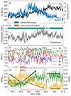 |
Fig. 1. Solar wind sample from 2006. (a) Solar wind proton velocity and density measurements, at 64-sec cadence. (b) Solar wind proton temperature measurements, at 64-sec cadence. Plasma types are based on Xu & Borovsky (2015), calculated at a 12-min cadence. (c) Twelve-minute averaged solar wind magnetic field measurements. The B components are in geocentric solar ecliptic coordinates. (d) avQ of Fe and O with uncertainties at a 12-min cadence. The arrows indicate trends of the variation in the avQ. The red rectangle marks an anticorrelated structure, which is discussed in Sect. 3.2. |
This work uses a recently developed tool that takes timescales and temporal lags into consideration (Gu et al. 2024) in order to identify unique time periods where the rise or fall of avQFe and avQO are anticorrelated (e.g., the time period marked by the red dashed-dotted lines in panel d of Fig. 1). We refer to such time periods as anticorrelated structures. Other solar wind parameters, including those shown in Fig. 1, within these structures are analyzed as well. We describe the data in Sect. 2, we introduce the identification procedure in Sect. 3.2, and we show statistical results in Sect. 4. A list of all identified anticorrelated structures is provided in the appendix.
2. Data
This work uses multiple data products from different instruments on board ACE Stone et al. 1998). The heavy ion data were measured at 12-min time resolution by SWICS (Gloeckler et al. 1998), and the data we use in this work are from 2001 to 2010. SWICS combines three measurement techniques (energy per charge, time of flight, and total energy) to determine an ion’s speed, mass, and charge. A subset of the data is available as high-resolution pulse-height analyzed (PHA) data, and a detailed and extensive description of the data analysis procedure applied to the PHA data is given in Berger’s PhD thesis (Berger 2008). The charge-state distributions of Fe (from Fe7+ to Fe16+) and O (from O6+ to O8+) are used to calculate the individual avQ. The charge-state distribution data provided by the ACE Science Center are at a 2-hour cadence and thus not suitable for the work presented here that investigates short-term variations. Magnetic field data comes from the Magnetometer (MAG; Smith et al. 1998) at 16-sec time resolution. Solar wind plasma data comes from the Solar Wind Electron Proton Alpha Monitor (SWEPAM; McComas et al. 1998) at a 64-sec time resolution. We used 4-min field-plasma merged data to calculate the plasma beta value. We used 12-min plasma data (synchronized to SWICS data) to determine the solar wind plasma type. The data sets from SWEPAM and MAG are provided by the ACE Science Center1.
The ICMEs analyzed in this work are listed by Cane & Richardson (2003) and Richardson & Cane (2010), and by the ACE Science Center2 (known as the R & C list). We used the Xu & Borovsky (2015) scheme, which categorizes the solar wind measured at 1 AU into the following four plasma types: streamer-belt-origin, coronal-hole-origin, sector-reversal-region, and ejecta. It is based on three parameters, proton specific entropy, proton Alfvén speed (VA), and proton temperature – heavy ion signatures are not considered.
3. Methods
In this section we first present a solar wind sample where at least one anticorrelated structure can be clearly observed. Then the identification procedure is introduced in detail, using this presented solar wind sample as an example.
3.1. An example
Figure 1 shows solar wind properties on the timescale of ∼0.5 day. Solar wind speed and density are shown in panel a, temperature is in panel b, and magnetic field is shown in panel c. Plasma parameters are shown at the SWEPAM time resolution of 64 seconds, while the magnetic field has been smoothed with a 12-minute window. Panel d shows avQFe and avQO. One can clearly see that avQFe and avQO do not always strictly follow the positive correlation obtained at large timescales. The arrows in panel d mark the rise or fall of avQ of Fe and O, which clearly have different timescales and unique non-zero temporal lags.
The variations in avQFe and avQO are complex. While avQFe and avQO are positively correlated before DOY 59.8, they are anticorrelated until DOY 60.4, after which avQFe declines and then remains constant, while avQO continues to decrease until it reaches a constant value later than avQFe. The avQ variations are not necessarily linear in time. Thus, in this work, we use the Spearman’s rank correlation (ρ), which does not rely on the assumption of linear relationships and studies the monotonicity3 of variations in avQ.
During this example time period, the solar wind proton velocity and temperature were generally increasing, while the proton density had a peak around day of year (DOY) 60.2, which is likely due to compression. After this peak, the density dropped continuously. The behavior of the magnetic field is more complex. Although Bx and the total strength, |B|, are relatively stable, the direction of the magnetic field vector fluctuates in the y-z plane (see By and Bz in panel c). This period is very likely related to a stream interaction region (SIR) between two slow solar wind streams, with almost all of the plasma being of streamer-belt-origin (Xu & Borovsky 2015).
3.2. Identification procedure
The identification of structures with anticorrelated avQ of Fe and O and their respective start and end times (ST and ET) was divided into five steps and is discussed in the following. Figure 2 shows the same time period as Fig. 1. The dash-dotted rectangle shown in Fig. 1 is also shown in Fig. 2. It marks the structure of interest where anticorrelated avQFe and avQO can be seen. Because we use Fig. 2 to develop the identification procedure step by step, we do not provide an overview of it here but discuss it as we develop the method. The method consists of five steps (1–5), which are described in more detail below. The first step searches the entire data for potential candidates. In the second step, we determine a first or initial estimate of the ST and ET, which is then refined in steps 3–5. The final result consists of two estimates of ST and ET, which we call strong and weak solutions (Sstrong and Sweak).
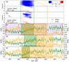 |
Fig. 2. Explanation of the procedure to identify anticorrelated structures. (a) Identification procedure step 1: The sliding-window cross-correlation map with a window size of 12 hours (60 data points). The black dashed line is the baseline where time lags are zero. Colored dashed lines mark the boundaries of the blue pattern and their time stamps on the x-axis, which is the visualization of the identification procedure step 2. (b) Sliding-window cross-correlation map with a window size of 6 hours (30 data points). (c) Measured avQFe and avQO. The estimated rise phase of avQFe is shaded in green, and the fall phase of avQO is shaded in orange. Purple solid lines and the area shaded in purple mark the extended time period of interest for this structure, representing step 3 of the identification procedure, while step 4 is then a pure mathematical calculation process. The red rectangle is the same as in Fig. 1 and is indicative only (i.e., it has no physical meaning). (d) Weak solution and related correlation coefficients defined in step 5 of the identification procedure. (e) Strong solution and related correlation coefficients defined in step 5 of the identification procedure. |
Step 1 of the procedure is to run a sliding-window cross-correlation scan (Gu et al. 2024) over the time period of interest, which in our case is ten years (2001–2010). We applied a 12-hour window4. This size was chosen based on an estimation of the average duration of the anticorrelated structures that we attempt to identify. Sliding-window cross-correlation maps were obtained, and we used these maps to identify anticorrelated structure candidates. Each candidate is represented by a blue pattern (ideally a parallelogram) near the τ = 0 line (i.e., the black dashed line in Fig. 2a) on the cross-correlation map. An example can be seen between the two dashed green vertical lines in panels a and b. The x-axis directly represents the center of the window in the avQFe signal, while τ in the y-axis represents the temporal lag between windows in the avQFe and avQO signals. A positive value means the window in the avQFe signal is ahead of the window in the avQO signal. The calculated Spearman’s rank correlation coefficients are color coded only for |ρ (avQFe[ST : ET],avQO[ST : ET])|≥0.5. Through this first step, we visually identified 153 candidates and repeated this selection process three times to avoid human errors and omissions. For instance, an anticorrelated structure candidate is visible in the cross-correlation maps in panels a and b.
Step 2 of the procedure involved finding an initial estimate for ST and ET for each candidate based on the boundaries of the parallelograms provided by the sliding-window cross-correlation map (similar to panel a). The boundary of each structure includes four time stamps: the start time, ST, and end time, ET, of both the avQFe and avQO signals (avQx[STx : ETx]). We refer to each boundary as a “solution” (S):
![Mathematical equation: $$ \begin{aligned} S = [\mathrm{ST} _{\rm Fe},\mathrm{ET} _{\rm Fe},\mathrm{ST} _{\mathrm{O}},\mathrm{ET} _{\mathrm{O}}]. \end{aligned} $$](/articles/aa/full_html/2024/12/aa51797-24/aa51797-24-eq1.gif) (1)
(1)
We call the solution estimated in this step the “initial solution” (Sini = [ST′Fe, ET′Fe, ST′O, ET′O]). The Sini is marked with vertical dashed lines (green: avQFe, orange: avQO) that extend into the correspondingly shaded regions in panel c. This Sini is affected by measurement uncertainties and random fluctuations, possibly from window sizes that do not perfectly fit the investigated event and different lengths in the avQFe and avQO signals. Thus, as a result of the uniform window size applied in step 1, the obtained parallelograms are not necessarily perfectly shaped parallelograms.
In order to refine the Sini, in step 3, we extend the time period defined by Sini by ±8 hours. These eight hours were chosen to include half the window width (six hours) and two hours of margin. This new, extended time period is shaded in purple in panel c and is bound by vertical solid purple lines.
Step 4 of the procedure is to create the solution space Ω. We note that Ω includes all S (with ST and ET within the time range defined in step 3) that meet all conditions from Eq. (2) to Eq. (7).
 (2)
(2)
![Mathematical equation: $$ \begin{aligned} |\rho (t,\mathrm{avQ} _{x}[\mathrm{ST} _{x}:\mathrm{ET} _{x}])|&\ge \rho _{\min }\end{aligned} $$](/articles/aa/full_html/2024/12/aa51797-24/aa51797-24-eq3.gif) (3)
(3)
![Mathematical equation: $$ \begin{aligned} \rho (t,\mathrm{avQ} _{\rm Fe}[\mathrm{ST} _{\rm Fe}:\mathrm{ET} _{\rm Fe}])\cdot \rho (t,\mathrm{avQ} _{\rm O}[\mathrm{ST} _{\mathrm{O}}:\mathrm{ET} _{\mathrm{O}}])& < 0\end{aligned} $$](/articles/aa/full_html/2024/12/aa51797-24/aa51797-24-eq4.gif) (4)
(4)
![Mathematical equation: $$ \begin{aligned} \rho (t,\mathrm{avQ} _{x}[\mathrm{ST} _{x}:\mathrm{ET} _{x}])\cdot \rho (t,\mathrm{avQ} _{x}[\mathrm {ST}{\prime } _{x}:\mathrm {ET}{\prime } _{x}])&>0\end{aligned} $$](/articles/aa/full_html/2024/12/aa51797-24/aa51797-24-eq5.gif) (5)
(5)
![Mathematical equation: $$ \begin{aligned} \{t \mid t \in [\mathrm{ST} _{\rm Fe}, \mathrm{ET} _{\rm Fe}]\} \cap \{t \mid t \in [\mathrm{ST} _{\mathrm{O}}, \mathrm{ET} _{\mathrm{O}}]\}&\ne \emptyset \end{aligned} $$](/articles/aa/full_html/2024/12/aa51797-24/aa51797-24-eq6.gif) (6)
(6)
![Mathematical equation: $$ \begin{aligned} \{t \mid t \in [\mathrm{ST} _{x}, \mathrm{ET} _{x}]\} \cap \{t \mid t \in [\mathrm {ST}{\prime } _{x}, \mathrm {ET}{\prime } _{x}]\}&\ne \emptyset . \end{aligned} $$](/articles/aa/full_html/2024/12/aa51797-24/aa51797-24-eq7.gif) (7)
(7)
The first condition (Eq. (2)) means that both signals have to be longer than tmin, which in this work is 2.4 hours (12 data points). Through a simplified hypothesis test (see Appendix A), structures lasting longer than 2.4 hours were found to have a probability lower than 5% that the anticorrelation between avQFe and avQO is caused by random fluctuations. Equation (3) requires the monotonicity of both signals with time to be significant, that is, ρ(time, signal) > ρmin, where ρmin is the significance level, which was chosen to be 0.8 for this test. This value strikes a good balance between a high and reliable correlation coefficient and a reasonable number of identified time periods. The number of solutions was not very sensitive to the exact choice of ρmin. Equation (4) ensures that avQFe and avQO are anticorrelated, and Eq. (5) ensures that avQx has the same sign of monotonicity as indicated by Sini. Equation (6) requires an overlap between the avQFe and avQO signals to strengthen the assumption that both signals come from nearly the same source region (or two regions that are close enough). If the two signals did not overlap, we would have to find a criterion for their maximum distance in time, which we considered to be too subjective. The last condition (Eq. (7)) requires that the signal of one heavy ion species overlaps with the corresponding initial signal in the Sini. It ensures that two neighboring time periods do not influence or interfere with each other. This step removed 50 candidates from the original list of 153.
Step 5 of the procedure is to determine the final solutions. Because the choice of ρmin is subjective, we present two solutions for each event. One solution is based on ρmin and called the “weak” solution (Sweak), while the other solution (Sstrong) is the one that resulted in the maximum ρ (t, avQFe)| and |ρ (t, avQO)|.
Panel d in Fig. 2 displays Sweak (see color-shaded region, green is for Fe and orange is for O), and the individual correlation coefficients are indicated along the bottom of the panel. The strong solution (Sstrong) is shown in panel e, where the individual correlation coefficients reach 0.89 and –0.94, as indicated along the bottom of the panel. In the following, the strong and weak solutions are both considered in the further analysis. We assumed that the more similar the properties of the two solutions are, the more reliable or well-determined the respective event is.
In summary, the determination of the start and end times of anticorrelated structures involved a visual survey (step 1), an initial estimate (step 2), and an adjustment procedure (steps 3 to 5). We note that ρ in step 1 compares avQFe with avQO but assumes their signals to have the same duration. However, this does not necessarily have to be the case. Because the calculation of the correlation coefficients between avQO and avQFe with different lengths would introduce more unnecessary assumptions, we instead chose to search for strong correlations (ρmin = 0.8) between the two signals and times separately.
4. Results
We identified 103 cases for which the avQFe and avQO signals show anticorrelated monotonic variations. Most of these anticorrelated structures were found during solar activity maximum (there are 90 cases from 2001 to 2004). We conducted a qualitative analysis, classifying all cases into several groups, and then we quantitatively analyzed the average proportion of different solar wind types in each group of cases (see Sect. 4.1). The solar wind kinetic properties are analyzed in Sect. 4.2, and related solar wind plasma types are studied in Sect. 4.3. Some aspects that might influence not only the measured avQ but also the cross correlations, such as cool-hot plasma mixing and heavy ion differential streaming, are evaluated in Sect. 4.4 and Sect. 4.5.
4.1. Number of cases and groups
We divided the 103 cases into two groups, namely ICME-related cases (shown as red stars in related figures) and non-ICME cases (shown as blue circles in related figures). The ICME-related cases are required to overlap with an ICME given in the R&C list. We also divided the events into two other groups according to the behavior of avQFe, namely “Fe-up” (shown as blue triangles in related figures) for cases in which avQFe increases with time and “Fe-down” (shown as orange inverted triangles in related figures) for cases in which avQFe decreases with time. This resulted in four groups, and they are analyzed in Sect. 4.2. The symbol of each group and the number of cases in each group are given in Table 1.
Number of cases in different groups and their unique markers used in this work.
The same symbols are used for the same group of cases in Figs. 3 and 5. In those figures, each anticorrelated structure is generally represented by two symbols of the same color. The filled (open) symbols correspond to the strong (weak) solution. The two symbols are connected by a straight line. Other solutions of this structure do not necessarily have to lie along this line. A large distance between the solid and empty symbols of a pair indicates a large difference between Sstrong and Sweak. The related case might be complex, and the calculated mean value could be unreliable because neither Sstrong nor Sweak is representative in that case.
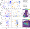 |
Fig. 3. Kinetic properties of identified anticorrelated structures in different groups. (a)/(b) Monotonicity of proton speed and temperature quantitatively described by Spearman’s rank correlation coefficients. (c) Two-dimensional distributions of proton speed and temperature for anticorrelated structures (scatter) and solar wind in 2001 (histogram). The bin width is 10 km/s and 5000 K. (d)/(e) Proton-proton collisional age and corresponding monotonicity. (f)/(g) Plasma beta value and corresponding monotonicity. (h) Two-dimensional distributions of proton-proton collisional age and plasma beta for anticorrelated structures (scatter) and solar wind in 2001 (histogram). The bin sizes are uniform on the logarithmic scale, for each bin, |
Table 1 shows that there are 87 cases that are not related to any of the R&C ICMEs, while only 16 cases are located inside an ICME. For non-ICME cases, there are 58 (66.7%) Fe-up cases and 29 (33.3%) Fe-down cases; that is, the ratio is two to one. However, the ratio is reversed in ICME-related cases, with five (31.3%) Fe-up cases and 11 (68.7%) Fe-down cases. The choice of strong or weak solutions (defined in step 5) as the basis for categorizing the cases does not affect this result.
The “O-early” category is a group of cases in which the systematic change in avQO begins before the change in avQFe, and the “O-late” category describes cases in which avQO starts to change after avQFe. These special cases are analyzed in Sect. 4.5, which also considers differential streaming. The definition of these two categories can be found in that section as well.
4.2. Kinetic properties
In Sect. 3.2, we describe how we selected the 103 time periods during which avQFe and avQO show an anticorrelated temporal behavior. In this section, we show how other plasma properties are correlated during these time periods.
Figure 3a shows the correlation coefficients of proton speed, with time plotted versus the correlation coefficients of proton temperature with time. These correlation coefficients indicate the robustness of the properties’ consistent increases and decreases. In the figure, one can clearly see two clusters around the lower-left and upper-right corners as well as a few cases that populate the rest of the possible space. The first cluster, where the velocity and temperature both increase with time, indicates stream interaction regions. The cluster where the velocity and temperature both decrease indicates rarefaction regions.
The clustering is also clear in panel b, where most Fe-up cases have an increasing proton speed and temperature, while many Fe-down cases have a decreasing proton speed and temperature, which means avQFe is generally positively correlated with solar wind speed and temperature. Considering that the avQO of Fe-up cases are dropping, this result is consistent with previous observations that avQO is generally anticorrelated with the solar wind speed. The proton density of the majority of Fe-up cases are decreasing (not shown here), and the kinetic properties indicate the solar wind is moving into a higher speed stream or a solar wind stream with more coronal-hole-like properties.
Panel c shows the occurrence of combinations of proton speed and temperature pairs for 2001. This serves as a reference background for the Fe-up and Fe-down cases that are plotted over this 2D histogram. The distributions of Fe-up and Fe-down cases differ from each other significantly (p < 1%) in the temperature distribution. Generally, Fe-up cases have a higher average proton temperature, possibly because Fe-down cases include more ICME-related cases, whose proton temperatures tend to be low (Wimmer-Schweingruber 2006). Furthermore, though the anticorrelation events appear to be distributed over a wide range of solar wind conditions, no cases were identified within the slowest solar wind (< 350 km/s).
Panels d and e show the correlation coefficients of proton-proton collisional age5 (acol) with time plotted versus acol for the different groups. The robustness of the monotonic increases or decreases of acol is indicated by ρ(time, acol). Most cases have a mean acol lower than one, indicating young and collisionless wind. The majority of the non-ICME cases and Fe-up cases also have a ρ(time, acol) < − 0.5, indicating acol decreases with time, while Fe-down cases have more cases with an increasing acol in comparison (more orange triangles on the top).
Panels f and g show the plasma beta (β), the ratio of the plasma pressure to the magnetic pressure, versus the correlation of β with time. Most of the anticorrelated structures have β < 1, and the β in the majority of the non-ICME cases do not have clear monotonic trends(|ρ|< 0.5). The β in ICME-related cases have more obvious monotonic trends, which might be related to the spacecraft crossing the fine-structure boundaries within the respective ICME. Panel h presents 2D distributions of acol and β for anticorrelated structures and solar wind in 2001 as a reference. The Fe-up and Fe-down cases differ slightly from each other in their β distributions (0.01 < p < 0.1), partly because Fe-down cases include more ICME-related cases with low β.
Apart from kinetic properties, we also investigated related magnetic field data. However, there is no clear evidence that shows that different groups have significantly different distributions in magnetic field strength or components and wave activity represented by B⊥/B. Thus, we do not show any related plots in this work.
According to Fig. 3, anticorrelated structures are more often seen in compression regions related to young, magnetically dominated solar wind. There is a positive correlation between avQFe and solar wind speed within these structures.
4.3. Solar wind plasma types
The positive correlations between avQFe in these structures and solar wind speed and temperature, as obtained in Sect. 4.2, motivated identifying whether the structures occur in the vicinity of stream boundaries. Therefore, we were interested in the context of the identified anticorrelated structures in the solar wind (related solar wind types).
According to the categorization of the solar wind following Xu & Borovsky (2015) and Sstrong, we found over 30 cases that have one dominant plasma type (see Table B.1, Nmajor plasma type = 1), which means the structure is likely located within that type of solar wind. Specifically, ejecta6 plasma dominates in five ICME-related cases. For the non-ICME cases, 19 are in streamer-belt-origin wind, ten cases are in coronal-hole-origin wind, two cases are in sector-reversal-region wind, and one case is dominated by ejecta plasma based on Sstrong. The example case in Sect. 3.2 (see Fig. 1b) is included in the 19 cases dominated by sector-reversal-region wind.
There are 43 (or 40 based on Sweak) cases with two major plasma types (Nmajor plasma type = 2), where a potential stream boundary is expected. Among the 43 cases, we further analyzed the detailed plasma type distributions in 35 non-ICME cases (with Sstrong) to check if an identified anticorrelated structure was located at the boundary of two different solar wind plasma origins. As shown in Fig. 4, each case is represented by one horizontal bar, and colors filled in that bar represent four different solar wind plasma types. The horizontal length of one certain colored region on one bar is the normalized duration of one certain type of solar wind. The serial numbers of cases (No.) are marked, and related cases can be found in the case list avaliable on Zenodo (see Data availability).
 |
Fig. 4. Detailed distributions of solar wind plasma types in non-ICME cases that have two or more major plasma types (Nmajor plasma type ≥ 2, based on Sstrong). Plasma types are based on Xu & Borovsky (2015), calculated on a 12-min cadence. The timeline has been normalized for each case; zero and one are min(STFe, STO) and max(ETFe, ETO). The serial numbers of cases (No.) are marked on the y-axis, and they correspond to the case list available at Zenodo (see Data availability). |
Panels a and b in Fig. 4 demonstrate the detailed distributions of solar wind plasma types in 35 non-ICME cases (25 Fe-up cases in panel a and 10 Fe-down cases in panel b, where Nmajor plasma type = 2). In those two panels, the second most abundant plasma type in some cases just has a rather low share (e.g., No.2 and No.60), or the second most abundant plasma type has a discontinuous (non-centralized) distribution (e.g., No.72). However, other cases suggest potential crossings of boundaries between different solar wind plasma origins, and the subjectivity introduced by defining Nmajor plasma type has little effect. For non-ICME&Fe-down cases (see panel b), most of them (eight out of ten) start within the streamer-belt-origin wind (blue) and end in a different plasma type. For non-ICME&Fe-up cases (see panel a), generally they end in either streamer-belt-origin wind (blue) or coronal-hole-origin wind (orange). If the end is mainly streamer-belt-origin wind, the start would not be coronal-hole-origin wind (e.g., No.32, No.33 and No.44). If the end is mainly coronal-hole-origin wind, then the start would most likely be streamer-belt-origin wind (e.g., No.64 and No.101).
If Nmajor plasma type > 2, then more than two plasma types are involved within the whole structure, indicating potential multiple stream interfaces. In panels c and d, the complex distributions of solar wind plasma types in 20 non-ICME cases are presented. Except for case No.31, the sector-reversal-region plasma, if it exists, only occurs in the first half of one case. Most coronal-hole-origin plasma occurs in the second half.
For these cases, we further calculated the mean proportions of the four different solar wind types in some different groups. Results are shown in the lower part of Table B.1 in the appendix, where Sstrong and Sweak were treated separately. No remarkable differences were found between the two kinds of solutions. Ejecta plasma and streamer-belt-origin plasma clearly account for the largest fractions in all groups. The proportion of ejecta plasma in non-ICME cases is much higher than that in ICME-excluded solar wind data. Outside of ICMEs from the R&C list, ejecta plasma could indicate undetected ICMEs, but the properties of these events fit better to dense and slow cool wind. Fe-up and Fe-down cases have similar results, wherein non-ICME&Fe-up cases have nearly twice the share of ejecta plasma than non-ICME&Fe-down cases.
To conclude, when combining Fig. 4 and Table B.1, one sees that about one-third of the non-ICME cases are predominantly associated with a single solar wind type. Another one-third are situated at the boundary between two solar wind types (streamer-belt-origin wind is highly involved), and the remaining one-third exhibit a rather strong mixture, making their solar source regions difficult to estimate. However, most of the cases with Nmajor plasma type ≥ 2 show a clear difference between the plasma type in the first and second half of the time period. Thus, the anticorrelated structures could be highly related to stream boundaries.
4.4. Charge state distributions and Fe16+
So far we have only considered the avQFe. Because this can be strongly influenced by an admixture of hot plasma (where hot is meant in the sense of hot coronal origin, which determines the freeze-in temperatures), we checked for the presence of Fe16+ in the time periods investigated in this paper. As Fe16+ has a Ne-like electronic configuration7, the fraction of Fe16+ is suitable for indicating the presence of a hot (high freeze-in temperature) population of Fe ions.
In Fig. 5a, we show the correlation of the number density of Fe16+ (normalized to overall Fe density) with time versus its normalized number density. One can easily see that the high fractions of Fe16+ (f > 10%) are mainly related to ICMEs, and the fractions of Fe16+ in those cases also exhibit a clear monotonic trend (|ρ|> 0.5 and more with a negative sign). Most non-ICME cases and a few ICME-related cases only have a small proportion of Fe16+. Therefore, the variations in avQFe are thus less likely influenced by Fe16+. Panel b shows the same parameters as in panel a but with the other two groups. Generally, the monotonic trend of the fraction of Fe16+ is consistent with that of avQFe. The cases of Fe-up occupy the middle and upper part of panel b, while the Fe-down cases are located mainly in the middle and lower part of this panel.
 |
Fig. 5. Detailed fractions of Fe16+ combined Fe charge states and charge-state distributions of Fe within Fe signals defined by STFe, ETFe. (a)/(b) Fractions of Fe16+ and related Spearman’s rank correlation coefficient. (c)/(d) Charge state distributions of Fe. (e)/(f) Summed fraction of Fe8+ and Fe9+ compared to the summed fraction of Fe11+, Fe12+, and Fe13+. The black dashed line is a linear fit for non-ICME cases. (g) Two-dimensional distribution of the two summed fractions in panel e/f for solar wind in 2001. The bin size is 0.02 in each direction. |
Panels c and d show the average charge-state distributions of Fe in different groups. For all groups, the dominant charge state is Fe10+, while the average distribution for solar wind in 2001 peaks at Fe9+, indicating that a slight extra heating process could be common among plasma in anticorrelated structures compared to normal solar wind. However, anticorrelations in avQ are also easier to detect if the change in avQ is higher. Therefore, this might also be a selection effect. In the panels, variations in the charge-state distributions are indicated by vertical bars (one standard deviation). Large error bars indicate that very different distributions of the Fe charge states contribute to different cases.
To further test for a possible admixture of hot or cold plasma, we plotted the summed fractions of Fe(11 + ,12 + ,13 + ) versus the summed fractions of Fe(8 + ,9 + ) in Fig. 5e–g. These plotted ions are typical in the non-ICME solar wind, and therefore we expected to see a straight line if the selected time periods sample the normal solar wind, as is indeed the case. The outliers are the ICME-related cases. The dashed black line was fitted to the non-ICMEs and is given by the following relation:  . Both solid and empty symbols were used in the fit. Based on the ionization equilibrium assumption, such a linear relationship can be obtained for Fe ions around a typical coronal temperature (∼1 MK with a Maxwell electron distribution) (Dzifčáková et al. 2015, 2021). Remarkably, the distribution of the solar wind time periods investigated in this paper are much narrower than that of the average solar wind that is shown in panel g8.
In summary, Figure 5 indicates that the variations in avQFe caused by the cool-hot plasma mixture effects are very limited. This is because hot plasma is rare and the summed fraction of Fe8 + ,9 + ,11 + ,12 + ,13+ is stable. In other words, the ejections of Fe ions with a freeze-in temperature outside the typical coronal temperature range (e.g., nanoflare- or microflare-associated small and unrecorded ICMEs) are unlikely to be related to most of the anticorrelated structures here.
4.5. Differential streaming of heavy ions
The temporal lags between the systematic rise or drop of avQFe and avQO might be caused by the differential streaming between Fe and O. However, as stated in Sect. 3.2 in steps 4 and 5, no optimal solution can be found for one case. Thus, discussing specific temporal lags calculated from any single solution from Ω is problematic because a single pair of ST and ET is not representative enough for one avQ signal due to the following factors: different signal-to-noise ratio in O and Fe signals, measurement uncertainties in general, and different lengths of two signals, which complicates computing the correlation coefficient directly. Therefore, when investigating the differential streaming between Fe and O, we only considered O-early9 and O-late cases, where the signs of the temporal lags are more reliable because the whole Ω is considered.
There are 37 cases for which the O signal starts earlier, and these cases are almost evenly distributed among the Fe-up (19) and Fe-down (18) cases. Only seven cases show a later O signal (see the legend at the top of Fig. 6 for the symbol usage).
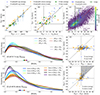 |
Fig. 6. Average velocity and 1D velocity distributions of individual ion species for different groups. We calculated VFe within the Fe signals ([STFe, ETFe]), and VO was calculated within O signals ([STO, ETO]). (a) Bulk speeds of Fe and O ions. (b) Differential speeds between the bulk of Fe and O ions and the local protons. (c) Two-dimensional distribution of the differential speeds between the bulk of Fe and O ions and the local protons. The averages of distributions in panel b are marked here. The bin width is 1 km/s in both directions. (d)/(f) Kernel density estimation functions of |δV|/VA for individual ion species in all Fe-up or Fe-down cases based on Sstrong. The peaks of distributions are marked by crosses. Pentagons above the x-axis mark the average δV of the individual charge states. The uncertainties of probability density were obtained based on a bootstrap method (Efron 1979) and are represented by shaded areas. (e)/(g) Differential speeds of different ion species. |
We used  to represent the bulk speed of O ions and
  for that of the Fe ions because they are the most abundant charge states for O and Fe in the solar wind. Figure 6a shows the bulk speeds of Fe and O ions in O-early and O-late cases based on Sstrong. The results related to Sweak are similar, so they are omitted here in order to better illustrate the bulk speed uncertainties, which are the standard deviations of the bulk speed within Fe or O signals. The bulk speeds of Fe and O ions were calculated for the time intervals defined by (STFe, ETFe) and (STO, ETO), respectively.
Examination of individual time series (not shown here) revealed that for many cases, the differential streaming is not observed during the complete event. Among all 103 cases, about 26 cases show differential streaming (heavy ions to protons) throughout the whole structure, while also about 26 cases show no clear differential streaming. The onset of differential streaming also does not always coincide with the start of the weak nor the strong solution. This section only presents statistical results.
In panel a, O-late cases (see green diamonds) have a relatively low speed compared to O-early cases (triangles). Two O-late cases have an O bulk speed lower than Fe, which is a possible reason for the later STO identified. However, the other five O-late cases have a similar O and Fe bulk speed or even slightly faster O ions. Such differential speeds would prevent a later beginning of the O signal. For the O-early cases, there is no clear evidence that this earlier onset is caused by O streaming faster than Fe. We note that O-early&Fe-down cases generally have O ions slightly faster than Fe ions (see orange triangles above the diagonal), while O-early&Fe-up cases generally have O slower than Fe, though the linear fits for orange and blue triangles are not significantly different if the errors are considered. Therefore, we consider the bulk speeds of Fe and O to be similar even in the high velocity range, where differential streaming is expected to be stronger (Berger et al. 2011). The large error bars in panel a also reflect the variability of the differential streaming during each event.
Panel b shows the differential speeds between the bulk of heavy ions and protons (within Fe signals or O signals, same as what we did in panel a). A positive differential streaming is common for Fe and O ions. Moreover, no matter whether they are O-early or O-late, O ions are almost evenly distributed around the diagonal.
The O-early&Fe-up cases (blue) tend to have stronger differential streaming than the O-early&Fe-down and O-late cases (orange and green). These average values are also plotted as crosses in panel c and were calculated based on the combined distribution of Sstrong and Sweak in panel b.
The values for the differential streaming in the events reported here lie within the normal distribution of the solar wind, as shown in panel c.
The results in panels a, b, and c show that heavy ion differential streaming between Fe and O is common in anticorrelated structures and not significantly different than the average solar wind. It cannot fully explain the identified temporal lags between STFe and STO, at least half of the cases have a heavy ion differential streaming that would prevent the formation of the identified temporal lags, where O ions move slower but are detected earlier.
We further analyzed the differential streaming between the same element but with different charge states, which could affect the detected significance of the monotonic trends of the variations in avQ because such differential streaming could change the spatial distribution of ions at different ionization levels. Panels d and f demonstrate the kernel density estimation (Rosenblatt 1956; Parzen 1962) functions of all  and
and  (differential speeds to local proton speed) divided by local Alfvén speed in all Fe-up or Fe-down cases based on Sstrong. In the differential velocity calculation (δV), each
  and
and  is the average velocity based on its velocity distribution function from the instrument during one detection period (12 min). The more counts the instrument records, the more reliable the velocity distribution function and the estimated velocity would be. In order to guarantee the reliability of δV, we required a minimum count of five for individual Fex+ and Ox+ during each detection period. The uncertainties of the probability density were obtained based on a bootstrap method with a bootstrap sample number of 100 (Efron 1979). The temporal structure of the differential streaming during each event sensitively influences the shape of these curves.
The Fe ions and O ions in Fe-up cases (see panel d) flow along the interplanetary magnetic field at velocities that are smaller than the local Alfvén speed. The average ratio is around 0.35. No big difference was observed between different Fe or O charge states for Fe-down cases (peaks are close). Regarding the average values, lower charged ions are slightly slower than higher charged ions. Positive differential streaming against protons is even weaker in Fe-down cases, especially for O (see left-shifted average values around 0.3 in panel f). The average |δV|/VA for Fe10+, Fe11+, and Fe12+ are very close (overlapped pentagons). The average |δV|/VA for both Fe-up cases and Fe-down cases are smaller than the typical value calculated based on two high speed streams in early 2008 by Berger et al. (2011), which is 0.55 ± 0.15.
Since a weak differential streaming between higher and lower charged ions was observed in some cases, we checked if this would influence the measured systematic changes in avQ. When the differential velocity between higher and lower charged ions are averaged for each event, Fe-up and Fe-down cases share very similar results, namely, the average  and
and  distributions show similar behavior and are concentrated in the y direction in panel e; higher charged Fe ions tend to flow slightly faster than the lower charged ones (
 ; see offset in the +x direction); and the average velocity of the three most abundant Fe charge states (Fe9 + ,10 + ,11+) are similar for most cases (concentration at the origin in panel g). Some cases, especially Fe-up cases, clearly show Fe11+ as being faster than Fe10+ and Fe10+ as being faster than Fe9+ (blue triangles in the gray shaded area in panel g).
The results in panels d, e, f, and g show that heavy ion differential streaming between different charge states is weak. The O6+ and O7+ ions can be considered as flowing at the same speed. Higher charged Fe ions tend to be slightly faster than lower charge states, especially in Fe-up cases. Such differential streaming would cause the spacecraft to detect higher charged Fe ions slightly earlier. Consequently, a drop of avQFe after the detection of the higher charged Fe ions is expected, which might not be the case when the bulk of Fe ions left the lower corona. More than half of the Fe-up cases have faster higher charged Fe ions (blue triangles in gray shaded region in panel g), but avQFe rises instead (the later, the more higher charged Fe ions there are). This means that such differential streaming is not the interpretation of the measured rise of avQFe.
In summary, Fig. 6 illustrates that the particle transport effects represented by heavy ion differential streaming, not only between O and Fe but also between different charge states, are limited. More than half of our identified anticorrelated structures have a temporal lag between STFe and STO or a systematic variation in avQFe that cannot be directly caused by the particle transport effects. However, we cannot rule out that instrumental uncertainties hide the influence of differential streaming. Nevertheless, the analysis of the differential speeds implies that the measured variations in avQ are possibly also related to the source region conditions. We discuss the particle transport effects, including some instrument effects, in Sect. 5.
5. Discussion
Iron and oxygen are two abundant heavy elements that are well resolved in the ACE/SWICS data. Thus, avQFe and avQO are reliable quantities, even if we neglected some rare charge states such as O5+ (Wimmer-Schweingruber et al. 1998) and Fe6 + ,17+. In a 12-min interval, these ions with rare charge states generally do not have enough counts to allow for a reliable estimate of the velocity distribution functions, and thus including these rare charge states would make the mean charge state less reliable. We verified that the choice of ions used to compute the average charge states does not affect our results by reproducing the work presented in this paper with avQFe calculated only using the more abundant charge states of Fe (from Fe8+ to Fe12+). We could still identify 96 cases out of the 153 candidates, and the main results reported in Sect. 4 remain valid.
However, in the identification procedure (see Sect. 3.2), uncertainties of avQFe and avQO are not considered directly. This could lead to the identification of potential structures with an avQ variation amplitude that is not significant compared to the measurement uncertainties. We checked the Fe signals separately based on Sstrong and Sweak, and more than 90% of the cases have a scale of avQ variations larger than twice the mean error of avQ (98 cases for Sstrong and 95 cases for Sweak). For the O signals, the values are 96 for Sstrong and 98 for Sweak. Generally, the identified scale of avQ variations is larger than the measurement uncertainties, making the identification procedure more reliable.
Uncertainties of avQFe and avQO also strengthen the necessity of creating Ω instead of seeking one optimal solution for each case. The reasons for not using the overall average solution S the solution space Ω are that the shape of Ω may be irregular and the density of S inside Ω is not uniformly distributed. Thus, the average is not necessarily the optimum solution. However, a pair of Sstrong and Sweak is sometimes still not good enough to represent the ST and ET of one structure. As shown in Fig. 3, the kinetic properties can be very different between Sstrong and Sweak (a long connection line), and they can even have distinctly different signs of monotonic trends in a few cases. Those cases can also have larger fluctuations in avQ. In this situation, neither Sstrong nor Sweak might be representative. We still kept such cases in our list because the existence of an anticorrelated structure is clear, though the boundaries are vague. The inability to define an optimal S in the solution space Ω is one limitation in our identification procedure, leading to uncertainties in the subsequent analysis.
Another limitation of our identification procedure is that we used a fixed manually chosen window size (12 hours), which is a compromise between the fluctuation scale and the target structure scale. For the current 103 cases, the averaged timescales for Fe and O signals are 6.2 hours and 11.1 hours (both based on Sstrong; timescales are 8.3 hours and 10.9 hours based on Sweak). The O signals tends to be longer than the Fe signals, possibly because avQFe is more variable in the solar wind and has a worse signal to noise ratio. Nevertheless, we could have missed some even shorter anticorrelated structures in the identification procedure step 1.
The fractions of Fe16+ are low in non-ICME cases, as shown in Fig. 5, indicating that there is no strong heating process involved. The summed fraction of Fe8 + ,9 + ,11 + ,12 + ,13+ is highly stable, indicating that the mixture of Fe ions with very different freeze-in temperatures caused by local occasional activities is unlikely. In that case, for example, the rise of avQFe is more likely related to an overall slight heating at the freeze-in height. The observed (time-delayed) anticorrelations could also be caused by different timescales to reach the ionization equilibrium in the respective regions or heights in the corona.
The particle transport effects are also limited as shown in Fig. 6. During their journey toward the spacecraft, the velocity of heavy ions is not a constant value. Other local structures such as shocks, turbulence, and wave-particle interactions play a role in generating differential streaming. A recent statistical work using data with 1-hour time resolution from ACE claims that various heavy ions always flow at the same bulk speed (Zhang et al. 2024). In our work, higher resolution data reveal that certain differential bulk speeds of Fe and O do exist in some anticorrelated structures. But the temporal lags that cannot be completely explained by Fe-O differential speeds indicate that the variations in source region conditions at different coronal heights might happen at different times. However, if the differential bulk speed of Fe and O is so large or lasts so long that the Fe signal and O signal detected at 1 AU already have no overlapping timestamps, the structure would be neglected by our identification procedure.
In addition, even though the differential streaming between ions with different charge states is also not obvious, there is a selection bias. If the differential streaming between ions with different charge states is strong, the avQ averaged over each case would contain more fluctuations. Consequently, the correlation between two avQ signals would be weakened, making the identification of the structure less likely. As a result, our identification procedure might miss some potential structures that are influenced by such transport effects and make the transport effects appear weak in the remaining structures. This is the selection bias. Thus, our identification procedure certainly underestimated the actual number of anticorrelated structures in the solar wind.
Since mixture effects and particle transport effects are not sufficient to explain all of our currently identified structures, anticorrelated variations in avQ are likely at least in part related to source region conditions, including temperature, electron density, electron distributions, and ionization equilibrium state.
Taking Fe-up cases as an example, according to Fig. 3, when the solar wind becomes younger (lower acol) and faster (shifting from the quiet Sun to coronal holes), its source region could have opposite variation trends at different heights. At lower corona (∼1.3 solar radii), O ions experience a cooling down process, while at higher corona (∼5 solar radii), Fe ions experience a heating process. Such variations do not necessarily happen at the boundaries of different solar wind types. They could be within one single type (19 cases occur within streamer-belt-origin wind and 10 cases within coronal-hole-origin wind; see Table B.1). Additionally, it is interesting to note that O signals generally begin earlier than Fe signals (37 O-early versus seven O-late), suggesting that changes in the corona may typically start in the lower corona, with some delay before affecting regions at higher freeze-in heights. This delay might be linked to electron movements.
It is known that the ionization state of heavy ions is a useful diagnostic in the characterization of different solar wind source regions. One point of view from Lepri et al. (2013) states that avQ cannot be used as an absolute discriminator of solar wind source. Our results indicate that including charge-state distribution information of more ions would probably lead to a better characterization of the source region. Furthermore, the source region itself could be very different at different heights. However, current solar wind models have just barely started to treat different corona heights separately, so potential energy-electron transfer along the vertical direction beyond 1.3 solar radii might have been ignored for a long time.
6. Conclusions
Using data from SWICS on ACE, we identified 103 time periods between 2001 and 2010 (mostly during solar maximum) where we observed anticorrelated rises and falls of the average charge states of Fe and O, avQFe and avQO. To our knowledge, such anticorrelated structures have never before been reported. We find that mixture effects and transport effects (such as differential streaming) alone cannot explain the observed anticorrelations. This suggests that varying conditions in the source region, particularly in the vicinity of stream boundaries, are the causes of the observed anticorrelations. We find that there are more anticorrelated structures in which avQFe increases with time in the non-ICME wind, while more structures in ICMEs tend to show a decrease of avQFe with time. The anticorrelated increases (decreases) between avQFe and avQO are also highly related to solar wind speed, temperature, and collisional age. About two-thirds of non-ICME anticorrelated structures are identified near at least one stream boundary.
In situ measurements of heavy ions at a closer distance from Solar Orbiter (Müller et al. 2020; Owen et al. 2020) are expected to identify and reveal more details of such structures because of the higher time resolution and higher heavy ion density. The Solar Orbiter Archive provides measurements of Fe8+ to Fe12+ from the Heavy Ion Sensor that is part of the Solar Wind Analyser Owen et al. (2020). Our work demonstrates, using ACE data, that the currently available Heavy Ion Sensor data – though limited to a few charge states – is sufficient to identify similar anti-correlated structures.
Data availability
The entire table listing the 103 anticorrelated structures identified in this work is available at the Zenodo on https://doi.org/10.5281/zenodo.14055494.
http://www.srl.caltech.edu/ACE/ASC/level2 (Retrieved 1 August 2023).
http://www.srl.caltech.edu/ACE/ASC/DATA/level3/index.html (Retrieved April, 21, 2022).
We use this word to indicate an overall monotonic trend that may be superimposed by random fluctuations.
Other window sizes ranging from 3 to 60 hours are applied to verify that the 12-hour results are not affected by the window-size selection. The reader may get an impression of the variability by comparing panels a and b of Fig. 2.
The term acol is a measure of the number of collisions experienced by the expanding solar wind plasma, which has been proposed as an ordering parameter for the solar wind (Kasper et al. 2008; Maruca et al. 2013; Tracy et al. 2016). It is defined as the ratio of the transit time of the solar wind (from the source region to the spacecraft) to the mean time between Coulomb collisions.
The “ejecta plasma” in Xu & Borovsky (2015) does not uniquely identify ICME plasma; “ejecta plasma” covers about 63% of ICME plasma defined by Cane & Richardson (2003) and also includes very dense and slow cool wind (Sanchez-Diaz et al. 2016). For example, the eject plasma in cases No.18 and No.52 have a lower avQFe than the streamer-belt-origin plasma ahead.
That is, it is stable and abundant at high temperatures.
Data plotted in panel g require a minimum count of three for each individual Fex+ to guarantee the reliability of the calculated number density, as the variability of the summed fractions from counting statistics is thus reduced.
“O-early” means over 95% of the S in Ω have STFe > STO.
Acknowledgments
This work is supported by China Scholarship Council (CSC) under the file number: 202106400008. Verena Heidrich-Meisner is supported by German Space Agency (DLR) grant number 50OC2104.
References
- Asbridge, J. R., Bame, S. J., Feldman, W. C., & Montgomery, M. D. 1976, J. Geophys. Res., 81, 2719 [NASA ADS] [CrossRef] [Google Scholar]
- Berger, L. 2008, Ph.D. Thesis, Kiel University, Germany [Google Scholar]
- Berger, L., Wimmer-Schweingruber, R. F., & Gloeckler, G. 2011, Phys. Rev. Lett., 106, 151103 [NASA ADS] [CrossRef] [Google Scholar]
- Cane, H. V., & Richardson, I. G. 2003, J. Geophys. Res.: Space Phys., 108, 1156 [NASA ADS] [Google Scholar]
- Dere, K. P., Landi, E., Mason, H. E., Monsignori Fossi, B. C., & Young, P. R. 1997, A&AS, 125, 149 [NASA ADS] [CrossRef] [EDP Sciences] [Google Scholar]
- Dzifčáková, E., Dudík, J., Kotrč, P., Fárník, F., & Zemanová, A. 2015, ApJS, 217, 14 [CrossRef] [Google Scholar]
- Dzifčáková, E., Dudík, J., Zemanová, A., Lörinčík, J., & Karlický, M. 2021, ApJS, 257, 62 [CrossRef] [Google Scholar]
- Efron, B. 1979, Ann. Stat., 7, 1 [Google Scholar]
- Feng, X., Yao, S., Li, D., Li, G., & Yan, X. 2018, ApJ, 868, 124 [NASA ADS] [CrossRef] [Google Scholar]
- Geiss, J., Gloeckler, G., von Steiger, R., et al. 1995a, Science, 268, 1033 [Google Scholar]
- Geiss, J., Gloeckler, G., & von Steiger, R. 1995b, Space Sci. Rev., 72, 49 [NASA ADS] [CrossRef] [Google Scholar]
- Gloeckler, G., Cain, J., Ipavich, F. M., et al. 1998, Space Sci. Rev., 86, 497 [NASA ADS] [CrossRef] [Google Scholar]
- Gopalswamy, N., Mäkelä, P., Akiyama, S., et al. 2013, Sol. Phys., 284, 17 [NASA ADS] [CrossRef] [Google Scholar]
- Gruesbeck, J. R., Lepri, S. T., Zurbuchen, T. H., & Antiochos, S. K. 2011, ApJ, 730, 103 [NASA ADS] [CrossRef] [Google Scholar]
- Gu, C., Yao, S., & Dai, L. 2020, ApJ, 900, 123 [NASA ADS] [CrossRef] [Google Scholar]
- Gu, C., Heidrich-Meisner, V., Wimmer-Schweingruber, R. F., & Yao, S. 2023, A&A, 671, A63 [NASA ADS] [CrossRef] [EDP Sciences] [Google Scholar]
- Gu, C., Heidrich-Meisner, V., & Wimmer-Schweingruber, R. F. 2024, A&A, 684, A125 [NASA ADS] [CrossRef] [EDP Sciences] [Google Scholar]
- Heidrich-Meisner, V., Peleikis, T., Kruse, M., Berger, L., & Wimmer-Schweingruber, R. 2016, A&A, 593, A70 [NASA ADS] [CrossRef] [EDP Sciences] [Google Scholar]
- Henke, T., Woch, J., Schwenn, R., et al. 2001, J. Geophys. Res.: Space Phys., 106, 10597 [NASA ADS] [CrossRef] [Google Scholar]
- Kasper, J. C., Lazarus, A. J., & Gary, S. P. 2008, Phys. Rev. Lett., 101, 261103 [Google Scholar]
- Kasper, J., Stevens, M., Korreck, K., et al. 2012, ApJ, 745, 162 [CrossRef] [Google Scholar]
- Kocher, M., Lepri, S.T., Landi, E., Zhao, L., & Manchester, W.B., IV 2017, ApJ, 834, 147 [NASA ADS] [CrossRef] [Google Scholar]
- Kocher, M., Landi, E., & Lepri, S. T. 2018, ApJ, 860, 51 [NASA ADS] [CrossRef] [Google Scholar]
- Landi, E., Alexander, R. L., Gruesbeck, J. R., et al. 2012a, ApJ, 744, 100 [NASA ADS] [CrossRef] [Google Scholar]
- Landi, E., Gruesbeck, J. R., Lepri, S. T., Zurbuchen, T. H., & Fisk, L. A. 2012b, ApJ, 761, 48 [NASA ADS] [CrossRef] [Google Scholar]
- Larrodera, C., & Cid, C. 2020, Sol. Phys., 295, 156 [NASA ADS] [CrossRef] [Google Scholar]
- Lepri, S. T., & Zurbuchen, T. H. 2010, ApJ, 723, L22 [Google Scholar]
- Lepri, S. T., Laming, J. M., Rakowski, C. E., & von Steiger, R. 2012, ApJ, 760, 105 [NASA ADS] [CrossRef] [Google Scholar]
- Lepri, S. T., Landi, E., & Zurbuchen, T. H. 2013, ApJ, 768, 94 [NASA ADS] [CrossRef] [Google Scholar]
- Maruca, B. A., Bale, S. D., Sorriso-Valvo, L., Kasper, J. C., & Stevens, M. L. 2013, Phys. Rev. Lett., 111, 241101 [CrossRef] [Google Scholar]
- McComas, D. J., Bame, S. J., Barker, P., et al. 1998, Space Sci. Rev., 86, 563 [CrossRef] [Google Scholar]
- Müller, D., St. Cyr, O. C., Zouganelis, I., et al. 2020, A&A, 642, A1 [Google Scholar]
- Ogilvie, K. W., Coplan, M. A., & Zwickl, R. D. 1982, J. Geophys. Res., 87, 7363 [NASA ADS] [CrossRef] [Google Scholar]
- Owen, C. J., Bruno, R., Livi, S., et al. 2020, A&A, 642, A16 [EDP Sciences] [Google Scholar]
- Parzen, E. 1962, Ann. Math. Stat., 33, 1065 [Google Scholar]
- Richardson, I. G., & Cane, H. V. 2010, Sol. Phys., 264, 189 [NASA ADS] [CrossRef] [Google Scholar]
- Rivera, Y. J., Landi, E., Lepri, S. T., & Gilbert, J. A. 2019, ApJ, 874, 164 [NASA ADS] [CrossRef] [Google Scholar]
- Rodkin, D., Goryaev, F., Pagano, P., et al. 2017, Sol. Phys., 292, 90 [NASA ADS] [CrossRef] [Google Scholar]
- Rosenblatt, M. 1956, Ann. Math. Stat., 27, 832 [Google Scholar]
- Sanchez-Diaz, E., Rouillard, A. P., Lavraud, B., et al. 2016, J. Geophys. Res.: Space Phys., 121, 2830 [NASA ADS] [CrossRef] [Google Scholar]
- Schmidt, W. K. H., Rosenbauer, H., Shelly, E. G., & Geiss, J. 1980, Geophys. Res. Lett., 7, 697 [NASA ADS] [CrossRef] [Google Scholar]
- Smith, C. W., L’Heureux, J., Ness, N. F., et al. 1998, Space Sci. Rev., 86, 613 [Google Scholar]
- Song, H., & Yao, S. 2020, Sci. China Technol. Sci., 63, 2171 [CrossRef] [Google Scholar]
- Song, H. Q., Zhong, Z., Chen, Y., et al. 2016, ApJS, 224, 27 [NASA ADS] [CrossRef] [Google Scholar]
- Song, H. Q., Chen, Y., Li, B., et al. 2017, ApJ, 836, L11 [NASA ADS] [CrossRef] [Google Scholar]
- Stone, E. C., Frandsen, A. M., Mewaldt, R. A., et al. 1998, Space Sci. Rev., 86, 1 [Google Scholar]
- Tracy, P. J., Kasper, J. C., Raines, J. M., et al. 2016, Phys. Rev. Lett., 116, 255101 [NASA ADS] [CrossRef] [Google Scholar]
- von Steiger, R., Geiss, J., Gloeckler, G., & Galvin, A. B. 1995, Space Sci. Rev., 72, 71 [NASA ADS] [CrossRef] [Google Scholar]
- von Steiger, R., Schwadron, N. A., Fisk, L. A., et al. 2000, J. Geophys. Res., 105, 27217 [Google Scholar]
- Wimmer-Schweingruber, R. F. 2006, Space Sci. Rev., 123, 471 [NASA ADS] [CrossRef] [Google Scholar]
- Wimmer-Schweingruber, R. F., von Steiger, R., & Paerli, R. 1997, J. Geophys. Res., 102, 17407 [NASA ADS] [CrossRef] [Google Scholar]
- Wimmer-Schweingruber, R. F., von Steiger, R., Geiss, J., et al. 1998, Space Sci. Rev., 85, 387 [NASA ADS] [CrossRef] [Google Scholar]
- Wimmer-Schweingruber, R. F., von Steiger, R., & Paerli, R. 1999, J. Geophys. Res., 104, 9933 [CrossRef] [Google Scholar]
- Wimmer-Schweingruber, R. F., Crooker, N. U., Balogh, A., et al. 2006, Space Sci. Rev., 123, 177 [Google Scholar]
- Xu, F., & Borovsky, J. E. 2015, J. Geophys. Res.: Space Phys., 120, 70 [NASA ADS] [CrossRef] [Google Scholar]
- Zhang, X., Song, H., Zhang, C., et al. 2024, ApJ, 967, 118 [NASA ADS] [CrossRef] [Google Scholar]
- Zhao, L., Zurbuchen, T. H., & Fisk, L. A. 2009, Geophys. Res. Lett., 36, L14104 [NASA ADS] [CrossRef] [Google Scholar]
Appendix A: A hypothesis test for the minimum duration of the structure
There is a probability that random fluctuations cause an anticorrelation structure. Here we explain this "probability" a bit more. Assuming there is no temporal lag, then the probability that whether an anticorrelation we identified within a certain time period is significant (P ( ρ (avQFe[ST : ET], avQO[ST : ET]) ≤ −0.5)) and unlikely caused by random fluctuations, is related to the duration of this time period, ET − ST. It is easy to understand that the longer the time period is, the less likely the anticorrelation is caused by random fluctuations.
We randomly shuffle the measurements of avQ in year 2001, and use a sliding window to obtain a large number of time series pairs (defined by ST and ET) of avQFe and avQO. Then we calculate the correlation coefficients (ρ) and the fraction of those ρ ≤ −0.5. This fraction represents the probability that a significant negative correlation coefficient is due to random fluctuations. As shown in Fig. A.1, the window size is the number of data points. When the window size is larger than 12 (2.4 hrs), the P ( ρ (avQFe[ST : ET], avQO[ST : ET]) ≤ −0.5) is less than 5%. In that case, the null hypothesis that a 2.4 hours long anticorrelation structure is caused by random fluctuations has a 5% probability to be true. Thus each case has its own chance to be caused by random fluctuations, and we consider 0.05 as the significance level is sufficient.
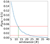 |
Fig. A.1. Probability of occurring significant anticorrelation, that is, P ( ρ (avQFe[ST : ET], avQO[ST : ET]) ≤ −0.5) versus window size. The red lines mark the significance level at 0.05 and 0.01. The green dashed line marks the window size of 12. |
Appendix B: Number of major solar wind plasma types
Number of major solar wind plasma types and the fraction of each type in anticorrelated structures in different groups.
All Tables
Number of major solar wind plasma types and the fraction of each type in anticorrelated structures in different groups.
All Figures
|
Fig. 1. Solar wind sample from 2006. (a) Solar wind proton velocity and density measurements, at 64-sec cadence. (b) Solar wind proton temperature measurements, at 64-sec cadence. Plasma types are based on Xu & Borovsky (2015), calculated at a 12-min cadence. (c) Twelve-minute averaged solar wind magnetic field measurements. The B components are in geocentric solar ecliptic coordinates. (d) avQ of Fe and O with uncertainties at a 12-min cadence. The arrows indicate trends of the variation in the avQ. The red rectangle marks an anticorrelated structure, which is discussed in Sect. 3.2. |
| In the text | |
|
Fig. 2. Explanation of the procedure to identify anticorrelated structures. (a) Identification procedure step 1: The sliding-window cross-correlation map with a window size of 12 hours (60 data points). The black dashed line is the baseline where time lags are zero. Colored dashed lines mark the boundaries of the blue pattern and their time stamps on the x-axis, which is the visualization of the identification procedure step 2. (b) Sliding-window cross-correlation map with a window size of 6 hours (30 data points). (c) Measured avQFe and avQO. The estimated rise phase of avQFe is shaded in green, and the fall phase of avQO is shaded in orange. Purple solid lines and the area shaded in purple mark the extended time period of interest for this structure, representing step 3 of the identification procedure, while step 4 is then a pure mathematical calculation process. The red rectangle is the same as in Fig. 1 and is indicative only (i.e., it has no physical meaning). (d) Weak solution and related correlation coefficients defined in step 5 of the identification procedure. (e) Strong solution and related correlation coefficients defined in step 5 of the identification procedure. |
| In the text | |
|
Fig. 3. Kinetic properties of identified anticorrelated structures in different groups. (a)/(b) Monotonicity of proton speed and temperature quantitatively described by Spearman’s rank correlation coefficients. (c) Two-dimensional distributions of proton speed and temperature for anticorrelated structures (scatter) and solar wind in 2001 (histogram). The bin width is 10 km/s and 5000 K. (d)/(e) Proton-proton collisional age and corresponding monotonicity. (f)/(g) Plasma beta value and corresponding monotonicity. (h) Two-dimensional distributions of proton-proton collisional age and plasma beta for anticorrelated structures (scatter) and solar wind in 2001 (histogram). The bin sizes are uniform on the logarithmic scale, for each bin, |
| In the text | |
|
Fig. 4. Detailed distributions of solar wind plasma types in non-ICME cases that have two or more major plasma types (Nmajor plasma type ≥ 2, based on Sstrong). Plasma types are based on Xu & Borovsky (2015), calculated on a 12-min cadence. The timeline has been normalized for each case; zero and one are min(STFe, STO) and max(ETFe, ETO). The serial numbers of cases (No.) are marked on the y-axis, and they correspond to the case list available at Zenodo (see Data availability). |
| In the text | |
|
Fig. 5. Detailed fractions of Fe16+ combined Fe charge states and charge-state distributions of Fe within Fe signals defined by STFe, ETFe. (a)/(b) Fractions of Fe16+ and related Spearman’s rank correlation coefficient. (c)/(d) Charge state distributions of Fe. (e)/(f) Summed fraction of Fe8+ and Fe9+ compared to the summed fraction of Fe11+, Fe12+, and Fe13+. The black dashed line is a linear fit for non-ICME cases. (g) Two-dimensional distribution of the two summed fractions in panel e/f for solar wind in 2001. The bin size is 0.02 in each direction. |
| In the text | |
|
Fig. 6. Average velocity and 1D velocity distributions of individual ion species for different groups. We calculated VFe within the Fe signals ([STFe, ETFe]), and VO was calculated within O signals ([STO, ETO]). (a) Bulk speeds of Fe and O ions. (b) Differential speeds between the bulk of Fe and O ions and the local protons. (c) Two-dimensional distribution of the differential speeds between the bulk of Fe and O ions and the local protons. The averages of distributions in panel b are marked here. The bin width is 1 km/s in both directions. (d)/(f) Kernel density estimation functions of |δV|/VA for individual ion species in all Fe-up or Fe-down cases based on Sstrong. The peaks of distributions are marked by crosses. Pentagons above the x-axis mark the average δV of the individual charge states. The uncertainties of probability density were obtained based on a bootstrap method (Efron 1979) and are represented by shaded areas. (e)/(g) Differential speeds of different ion species. |
| In the text | |
|
Fig. A.1. Probability of occurring significant anticorrelation, that is, P ( ρ (avQFe[ST : ET], avQO[ST : ET]) ≤ −0.5) versus window size. The red lines mark the significance level at 0.05 and 0.01. The green dashed line marks the window size of 12. |
| In the text | |
Current usage metrics show cumulative count of Article Views (full-text article views including HTML views, PDF and ePub downloads, according to the available data) and Abstracts Views on Vision4Press platform.
Data correspond to usage on the plateform after 2015. The current usage metrics is available 48-96 hours after online publication and is updated daily on week days.
Initial download of the metrics may take a while.