| Issue |
A&A
Volume 684, April 2024
|
|
|---|---|---|
| Article Number | A98 | |
| Number of page(s) | 14 | |
| Section | Extragalactic astronomy | |
| DOI | https://doi.org/10.1051/0004-6361/202348561 | |
| Published online | 09 April 2024 | |
Obscuration in high-redshift jetted quasi-stellar objects
1
INAF – Osservatorio Astronomico di Brera, Via Brera 28, 20121 Milan, Italy
e-mail: This email address is being protected from spambots. You need JavaScript enabled to view it.
2
DiSAT, Università degli Studi dell’Insubria, Via Valleggio 11, 22100 Como, Italy
3
International Centre for Radio Astronomy Research, Curtin University, 1 Turner Avenue, Bentley, WA 6102, Australia
4
Max Planck Institut für Astronomie, Königstuhl 17, 69117 Heidelberg, Germany
5
INAF – Osservatorio di Astrofisica e Scienza dello Spazio, Via Gobetti 93/3, 40129 Bologna, Italy
6
Dipartimento di Astronomia, Università di Bologna, Via Ranzani 1, 40127 Bologna, Italy
7
INAF – Istituto di Radioastronomia, Via Gobetti 101, 40129 Bologna, Italy
8
Dept. of Physics & Astronomy and Dept. of Computer Science, University College London, Gower Street, London WC1E 6BT, UK
9
Centro de Física da UC, Departamento de Física, Universidade de Coimbra, 3004-516 Coimbra, Portugal
Received:
10
November
2023
Accepted:
30
January
2024
Abstract
Context. Obscuration in high-redshift quasi-stellar objects (QSOs) has a profound impact on our understanding of the evolution of supermassive black holes across cosmic time. An accurate quantification of its relevance is therefore mandatory.
Aims. We present a study aimed at evaluating the importance of obscuration in high-redshift jetted QSOs, that is, active nuclei characterised by the presence of powerful relativistic jets.
Methods. We compared the observed number of radio-detected QSOs at different radio flux density limits with the value predicted by the beaming model on the basis of the number of oriented sources (blazars). Any significant deficit between observations and predictions of radio-detected QSOs can be caused by the presence of obscuration along large angles from the jet direction. We applied this approach to two sizeable samples characterised by the same optical limit (mag = 21) but with significantly different radio density limits (30 mJy and 1 mJy, respectively) and containing a total of 87 independent radio-loud 4 ≤ z ≤ 6.8 QSOs, 31 of which are classified as blazars.
Results. We found generally good agreement between the numbers predicted by the model and those actually observed, with only a marginal discrepancy at ∼0.5 mJy that could be caused by the sample’s lack of completeness. We concluded that we have no evidence of obscuration within angles 10–20° from the relativistic jet direction. We also discuss how the ongoing deep wide-angle radio surveys will be instrumental to testing the presence of obscuration at much larger angles, up to 30–35°. Finally, we suggest that, depending on the actual fraction of obscured QSOs, relativistic jets could be much more common at high redshifts compared to what is usually observed in the local Universe.
Key words: galaxies: active / galaxies: high-redshift / galaxies: jets / quasars: general
© The Authors 2024
 Open Access article, published by EDP Sciences, under the terms of the Creative Commons Attribution License (https://creativecommons.org/licenses/by/4.0), which permits unrestricted use, distribution, and reproduction in any medium, provided the original work is properly cited.
This article is published in open access under the Subscribe to Open model. This email address is being protected from spambots. You need JavaScript enabled to view it. to support open access publication.
1. Introduction
The study of the very first phase of supermassive black hole (SMBH) growth represents a critical step in understanding the galaxy’s early evolution (e.g., Heckman & Best 2014; Merloni 2016). To this end, a reliable and complete census of the accreting SMBH, that is, active galactic nuclei (AGN), at high redshifts is necessary (e.g., Bañados et al. 2016, 2022; Pacucci & Loeb 2021; Fan et al. 2022). For observational reasons, the study of accreting SMBHs at high redshift is mostly limited to the part of the population residing in unabsorbed objects, the so-called type 1 AGN, while SMBHs embedded in absorbed systems (type 2 AGN) typically elude observations. Up to now, these elusive objects were nearly beyond the capabilities of existing telescopes, except for a few possible examples (e.g., Endsley et al. 2022; Drouart et al. 2020). However, their detection is now becoming possible thanks to the James Webb Space Telescope (e.g., Yang et al. 2023). For these reasons, most studies of SMBH formation and evolution are still based on unobscured high-redshift AGN, and therefore, they are potentially biased. The assumption that the fraction of obscured AGNs at high redshift is equal to the one measured locally is too simplistic, since there are several pieces of evidence showing that the fraction of obscured sources significantly increases at high-z (see e.g., Zeimann et al. 2011; Moretti et al. 2012; Merloni et al. 2014; Aird et al. 2015; Gilli et al. 2022; Vijarnwannaluk et al. 2022; Yang et al. 2023).
The presence of a relativistic jet in AGN helps greatly in quantifying the importance of obscuration. When an AGN of this type is observed close to the jet direction, its emission is significantly boosted due to relativistic beaming, and the oriented nature of the source can be easily recognised. Such oriented sources are called blazars (see Urry & Padovani 1995 for a review). Notably, the particular orientation of blazars makes obscuration marginal since the jet is expected to clear out the path along the line of sight. From a statistically complete sample of blazars selected at a given radio limit, it is possible to study the impact of the circum-nuclear obscuring medium since the detection of a blazar with a given radio flux density implies the existence of a well-defined number of misaligned sources at lower flux densities (∼2Γ2, where Γ is the bulk Lorentz factor of the jet). When compared to predictions, a significant deficit of the observed misaligned sources implies the existence, at a certain critical angle, of an obscuration structure. Using this approach, Ghisellini & Sbarrato (2016) pointed out the possible presence of an almost 4π obscuring structure around the most luminous jetted AGN, although this result was quite uncertain, being based on a small sample of blazars.
We note that from the optical point of view, the class of blazars includes two different types of sources: (1) BL Lac objects that are characterised by featureless optical spectra and (2) flat-spectrum radio quasars (FSRQs), whose optical properties are similar to those observed in radio-quiet quasi-stellar objects (QSOs), as they are usually dominated by the accretion disc emission at these wavelengths. These two types of blazars are likely associated with two different classes of jetted AGN characterised by different physical properties probably connected to the accretion rate on the central SMBH (e.g., Tadhunter 2016). In this work, we only consider the class of FSRQs since BL Lac objects are not usually found at high redshifts (≥4), though the possible discovery of a BL Lac at z ∼ 6.57 has recently been claimed (Koptelova & Hwang 2022). Throughout the paper, we use the term ‘QSO’ to indicate an AGN with strong emission lines (EW > 5 Å) and/or clear evidence of the accretion disc emission in the optical spectrum regardless of its luminosity and/or the presence of a jet.
In this work, we use two sizeable flux-limited samples of high-redshift blazars to investigate the issue of obscuration in jetted QSOs in the early Universe by adopting a statistical approach similar to that described in Ghisellini & Sbarrato (2016). The first sample is the Cosmic Lens All Sky Survey (CLASS ) high-z QSO sample (Caccianiga et al. 2019; Ighina et al. 2019), which is characterised by a relatively high radio flux density limit (30 mJy) and an optical limit of mag = 21. The second sample is based on data from the Faint Images of the Radio Sky at Twenty-Centimeters (FIRST) Survey and has a much fainter radio flux density limit (0.5 mJy) but the same optical limit as CLASS. The combination of these two samples greatly increases the sensitivity of the method to absorption effects and, at the same time, improves the statistics, making our study more accurate.
In Sect. 2 we discuss the method used to derive the expected number of jetted QSOs from the observed number of oriented sources (blazars) in a flux-limited sample. We then apply this method to the CLASS sample in Sect. 3 and to the FIRST sample in Sect. 4. In Sect. 5, we discuss the expected improvements offered by new incoming surveys based on Square Kilometre Array (SKA) precursors and pathfinders. Finally, in Sect. 6, we summarise our conclusions.
In this paper, we use the magdrop defined as the magnitude in the AB system and corrected for Galactic extinction in the reddest filter of the dropout used to select the sources. This means the r-filter for 4 ≤ z < 4.5, the i-filter for 4.5 ≤ z < 5.4, the z-filter for 5.4 ≤ z < 6.3, and the y-filter for z ≥ 6.3 objects. By construction, magdrop corresponds to a quite narrow range of rest-frame wavelengths between ∼1250 Å and 1450 Å. Throughout the paper we assume a flat ΛCDM cosmology with H0 = 71 km s−1 Mpc−1, ΩΛ = 0.7 and ΩM = 0.3. Spectral indices are given assuming Sν ∝ ν−α.
2. Blazars versus misaligned sources: A test for obscuration
In the simplest version of the unified model (e.g., Antonucci 1993; Urry & Padovani 1995; Netzer 2015), QSOs are axis-symmetric sources that may appear either absorbed (type 2) or unabsorbed (type 1) depending on whether the line of sight intercepts an obscuring structure called dusty torus. In this picture, the aperture of the dusty torus determines the observed fraction of absorbed QSOs in a given sample. Thus, knowing the torus aperture is fundamental to accounting for the (unobserved) obscured population and to obtaining a reliable census of the entire population.
The presence of relativistic jets in a fraction of QSO greatly helps infer the source orientation and, therefore, assess the existence of an obscuring structure at a certain angle from the jet direction. In particular, the relativistic beaming makes oriented sources orders of magnitudes brighter than misaligned objects and, therefore, easily recognizable thanks to their ‘blazar properties’, such as a core-dominated flat spectrum radio emission, variability, and a strong X-ray emission with a flat photon index. Since beaming effects are maximised for angles within 1/Γ from the jet direction (Γ is the bulk velocity of the jet), a common assumption is that blazars are observed within this angle, though this statement should be considered valid in a statistical sense. We thus refer to Θb = 1/Γ as the ‘blazar angle’. This means that for each observed blazar, there should be 4π/Ωb ∼ 2Γ2 sources with the same intrinsic properties and with a jet randomly oriented, where Ωb is the solid angle corresponding to Θb1. Therefore, given the number of blazars observed in a certain volume of the Universe, it is possible to infer the total number of sources with the same properties within the same volume. The presence of obscuration at a certain viewing angle reduces the observed number of misaligned radio-emitting QSOs if we are selecting only unobscured (type 1) sources. The comparison between the predicted and the observed number of jetted type 1 QSOs can thus yield direct information on the impact of obscuration in the sample.
Real samples, however, are typically flux limited, and the situation is more complicated since beaming greatly boosts the fluxes of blazars, thus favouring their inclusion in the sample. For this reason, the non-blazar–blazar relative ratio observed in a flux-limited survey is, in general, significantly different from 2Γ2 and depends on several factors, including the survey limit(s) and the shape of the luminosity function (e.g., see discussion in Lister et al. 2019).
Ghisellini & Sbarrato (2016) developed a simple method to predict the expected number of misaligned sources in a flux-density limited sample on the basis of the observed fluxes of blazars selected in the same sample. In summary, given a sample with a flux density limit Slim and containing N blazars in a certain redshift interval, we expect to find, at the same flux limit and within the same redshift interval, a number (Ntot) of blazars plus non-blazars (i.e., with a misaligned jet) given by2
![Mathematical equation: $$ \begin{aligned} N_{\rm tot} \sim \sum _{i=1}^N{[2(\frac{S_i}{S_{\rm lim}})^{1/p} -1]}, \end{aligned} $$](/articles/aa/full_html/2024/04/aa48561-23/aa48561-23-eq1.gif) (1)
(1)
where the sum is calculated based on all the blazars selected in the survey and Si are their flux densities. The parameter ‘p’ appears in the beaming model and depends on the jet. For instance, if α is the radio spectral index of the emitting source, we expect p = 3 + α for a moving isotropic source and p = 2 + α for a continuous jet (see Appendix B of Urry & Padovani 1995 review paper for more details). It is worth noting that Eq. (1) does not depend on the value of Γ, and the only free parameter is p. This greatly reduces the uncertainties of the method.
We tested the validity of Eq. (1) via Monte Carlo simulations and found that it systematically overpredicts the number of sources by a factor ∼1.4 (see Appendix A). This is likely related to the fact that in the Ghisellini & Sbarrato (2016) work, all blazars are assumed to be observed at an angle exactly equal to 1/Γ rather than ≤1/Γ. If we take this effect into account and assume that blazars are observed at different angles within 1/Γ, Eq. (1) becomes (see Appendix A for its derivation)
![Mathematical equation: $$ \begin{aligned} N_{\rm tot} \sim \sum _{i=1}^N {\left[1.44\left(\frac{S_i}{S_{\rm lim}}\right)^{1/p} -1\right]}. \end{aligned} $$](/articles/aa/full_html/2024/04/aa48561-23/aa48561-23-eq2.gif) (2)
(2)
We use this formula throughout the paper.
Strictly speaking, the value of Ntot provided by Eq. (2) should be considered as a lower limit on the expected number of jetted high-z QSOs since it is computed only on the basis of the jet luminosity, neglecting the un-beamed extended emission of the source (such as that from the radio lobes). This effect can be particularly relevant when working with samples selected at low frequencies, where the extended emission is expected to be more important, while it should progressively become less relevant when moving to higher frequencies. When dealing with high redshift (z > 4) sources, where a typical observed frequency of 1.4 GHz corresponds to rest-frame frequencies above 7 GHz, the relevance of the extended components should be marginal. In addition, the extended radio emission is expected to be partially dumped by the interaction between the electrons in the jets and the photons from the cosmic microwave background (CMB; e.g., Ghisellini & Tavecchio 2009; Paliya et al. 2020; Ighina et al. 2021). In any case, in the analysis described in the next sections, we always use the peak flux densities rather than the total integrated flux densities in order to minimise the possible contribution from any extended emission.
After deriving and testing this method to estimate the expected number of type 1 jetted QSOs in a radio flux-limited sample, we could then apply it to real samples to see if the number yielded is consistent with the observations. A deficit of the observed number may suggest the presence of obscuration at a given angle from the jet direction. If the sample is large enough, we can even apply Eq. (2) at different flux densities. In this way it is also possible to infer the angle at which the obscuration occurs, as is shown in the next sections.
We first applied the method to the CLASS sample, which is characterised by a high radio flux limit compared to the optical one. We then built a sample with a much deeper radio flux density limit, thus containing more misaligned objects, making the comparison between predictions and observations more stringent.
3. The CLASS sample
The first sample we considered was the CLASS sample of high-z QSOs (Caccianiga et al. 2019; Ighina et al. 2019). This is a completely identified flux-limited sample of flat-spectrum sources with z ≥ 4 at the radio limit of 30 mJy at 5 GHz and magdrop ≤ 21 covering 13 120 sq. degrees of sky at high Galactic latitude (|bII|> 20°). The original complete sample was presented in Caccianiga et al. (2019) and contained 21 spectroscopically confirmed z > 4 QSOs, out of which 18 were classified as blazars on the basis of their X-ray emission (see Ighina et al. 2019 and the Sect. 4.1 for more details on the classification method). The CLASS sample has been used to obtain an accurate estimate of the space density of high-z blazars (Caccianiga et al. 2019; Ighina et al. 2021) and to track the evolution of the most massive SMBH (above 109 M⊙) hosted by jetted QSOs up to z ∼ 6 (Diana et al. 2022).
To this sample, we added two sources (J222032.5+002537 at z = 4.1960 and HZQ J142048.0+120546 at z = 4.0344), both classified as blazars (Sbarrato et al. 2015), that were not originally included because their radio spectrum between 1.4 and 5 GHz was steeper than 0.5 and therefore above the threshold used to define CLASS (αR ≤ 0.5)3 Therefore, the final sample we considered contains 23 sources: 20 classified as blazars and three classified as misaligned objects (see Table C.1). At first glance, this dominance of blazars in the CLASS sample could be considered evidence of the fact that obscuration plays an important role in hiding misaligned sources. However, as previously discussed, the actual fraction of blazars in a flux-limited sample depends on several factors, and by only using the method described in Sect. 2, we can establish whether the observed number is consistent or not with the expectations.
If we apply Eq. (2), where N = 20 is the total number of blazars and Si are their 5 GHz flux densities reported in Table C.1 (Col. 7), we predict the existence of 20–24 QSOs (using p = 3 and 2, respectively) in the same area and with the same radio and magnitude limits, that is, five misaligned sources at the most. This is fully consistent with what we observed. Therefore, the large fraction of blazars observed in the CLASS survey is not surprising, and it is simply due to the high radio-flux limit compared to the optical one, which favours the selection of sources with high radio-to-optical flux ratios (i.e., oriented sources).
The fact that CLASS is not very sensitive to sources observed at large viewing angles implied that we would only be able to test for the presence of obscuration at angles slightly above 1/Γ. In order to extend the test to larger angles, it was necessary to lower the radio-flux limit while keeping the same optical limit. Therefore, we began to select more sources with lower radio-to-optical flux ratio values that are likely observed at larger viewing angles. In the next section, we discuss the selection of a sample that is much deeper (by more that a factor 10) in the radio than CLASS but has the same optical limit.
4. The FIRST sample
In order to extend the analysis at lower flux densities, we considered the sample of z > 4 QSOs detected in the FIRST catalogue (Becker et al. 1995). The sample was selected by cross-matching FIRST sources with all the objects in the SDSS-DR17 database spectroscopically classified as ‘QSO’ with z ≥ 4 using the provided spectroscopic search tool4. We then complemented this search by considering all the known QSOs from the literature with a spectroscopically confirmed redshift above four using either the NASA/IPAC Extragalactic Database5 or SIMBAD6. To obtain a reliable quantification of the number of z > 4 QSOs, we restricted our analysis to a specific sky area (9 h ≤ RA ≤ 16 h, 0°≤ Dec ≤ 60°, |b|> 20°) where we expected that most of the z ≥ 4 and magdrop ≤ 21 QSOs have actually been identified thanks to the SDSS spectroscopy. We verified that in this area, which covers 5215 sq. degrees, all the high-z sources with mag ≤ 21 present in CLASS have an SDSS spectrum in the last data release. For this reason, we are confident that the completeness of the sample is high (> 90%), at least up to z ∼ 5.5. This is in agreement with the results from Schindler et al. (2017) showing that in this sky area and for relatively faint magnitudes (> 19), the QSO selection should be highly complete.
We visually inspected the SDSS spectra of all the z > 4 QSOs from DR17 falling in this sky area in order to confirm the redshift or exclude objects with a wrong z estimate (most of which were claimed to be at z > 5). In addition, we searched for all the sources in the literature that have been classified as z ≥ 4 QSOs (with a spectroscopic observation) in the same sky area. We thus obtained a list of 1330 spectroscopically confirmed z ≥ 4 QSOs with magdrop ≤ 21, 66 of which were detected in the FIRST catalogue ( mJy). Sixty-two of these objects have a spectrum from SDSS, while we found the spectrum for four sources in the literature (see Table C.1). Two of these (J090132.6+161506 at z = 5.63, Bañados et al. 2015, and J112925.3+184624 at z = 6.82, Bañados et al. 2021) are at z > 5.5, where the completeness of the SDSS is known to be lower. The other two objects (J101337.8+351849, Gloudemans et al. 2022 and J145224.2+335424, Stern et al. 2000) have a redshift below 5.5. Overall, the sources that were not found by the SDSS represent ∼6% of the sample (∼3% considering the 4 ≤ z ≤ 5.5 range), and this is consistent with the hypothesis that the SDSS spectroscopic sample is highly complete > 90%) in this area of sky and for sources in this range of redshift and magnitude.
Since the FIRST catalogue was produced using a 5 × rms threshold, it is possible to extend the sample down to lower flux densities using the FIRST radio data and searching for  mJy beam−1 (> 3 × rms) around the optical position of z > 4 QSO. This lower threshold is reasonable considering that we were ‘forcing’ the photometry towards a limited number of known positions and did not carry out a blind search, which was done in the original FIRST catalogue. Using this technique, we found seven additional sources with peak surface densities between 0.5 and 0.9 mJy beam−1. One of these sources (J133422.6+475033) has been also detected at 140 MHz in the Low Frequency Array (LOFAR) Two-metre Sky Survey (LoTSS; Gloudemans et al. 2022). The radio maps of these newly discovered radio detections are reported in Fig. 1. Since it is difficult to test the actual completeness of this extension at 0.5 mJy, we used the original sample at 1 mJy for most of the computations, while we used the extension only to reveal hints of possible trends at lower flux densities.
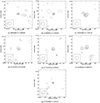 |
Fig. 1. Radio maps at 1.4 GHz from FIRST data of the seven high-z QSOs in the sample with peak flux densities between 0.5 and 0.9 mJy beam−1. These sources are not included in the FIRST catalogue. The levels were computed as −2, 2, 2.8, 4, 5.5, 8, ...times the rms (0.15 mJy beam−1). The central cross indicates the optical position of the high-z QSOs, while the beam size is reported in the bottom-left corner. |
In total, the final FIRST sample contains 73 z ≥ 4 radio-emitting QSOs with a peak flux density at 1.4 GHz ≥0.5 mJy beam−1 and magdrop ≤ 21. In Table C.1, these sources are flagged with the letter ‘F’. The 73 radio detections correspond to 5% of the total number of z ≥ 4 type 1 QSOs with mag ≤ 21 present in the considered sky area (1330).
There are nine sources in the FIRST sample in common with CLASS (i.e., all the CLASS high-z QSOs falling in the sky area covered by FIRST). Therefore, the two samples studied here contain a total of 87 independent z ≥ 4 jetted QSOs.
4.1. Blazar classification
In order to apply Eq. (2), it is necessary to recognise all blazars present in the FIRST sample. Historically, blazars with emission lines were identified with the class of FSRQs that are defined on the basis of their flat (αR < 0.5) radio spectrum. A flat spectrum is usually attributed to a source that is dominated by the self-absorbed emission from the core, that is, from the relativistically boosted, unresolved part of the jet (e.g., Urry & Padovani 1995). Often, the slope of the radio spectrum is evaluated on the basis of non-simultaneous flux densities measured at two different frequencies. Not only may variability affect the measure of the slope but also complex spectral shapes, such as peaked spectra, and they can lead to a misclassification of a source as FSRQ if only two points are used to characterize the spectrum. This is particularly true for high-z jetted QSOs that often show gigaherts-peaked spectra, possibly due to their young age (e.g., Frey et al. 2011; Momjian et al. 2021; Zhang et al. 2021; Belladitta et al. 2023). Moreover, at high redshifts, we usually cover the high frequency part of the radio spectrum where the core, which has a flat spectrum, can dominate the steep extended emission, even in moderately misaligned sources. This can be even more true considering that the extended emission can be dumped at high redshift due to the effect of the CMB, as mentioned in Sect. 2. For all these reasons, while the two-point radio spectrum can be effectively used to efficiently preselect high-z blazar candidates (e.g., Caccianiga et al. 2019), caution should be used when adopting the radio slope to classify a source, particularly when the spectrum is measured with non-simultaneous flux densities. In the near future, the availability of surveys, such as GLEAM-X (Wayth et al. 2018; Hurley-Walker et al. 2022), that can provide simultaneous spectra between 72 and 231 MHz (corresponding to rest-frame frequencies of 400 MHz–1.3 GHz at z = 4.5) for sources down to 5 mJy will allow for a more accurate spectral classification of high-z radio-emitting QSOs.
Alternatively (or in addition), high-resolution VLBI observations are often used to constrain the orientation of a high-z QSOs. In particular, the detection of a high brightness temperature (Tb) above the equipartition limit, is usually considered a robust way to classify a source as blazar (Frey et al. 2008, 2010, 2018; Gabanyi et al. 2015; Coppejans et al. 2016; Spingola et al. 2020; Liu et al. 2022; Krezinger et al. 2022). Unfortunately, for sources of a few millijansky (or below), the maximum baseline available on Earth is not long enough to put a stringent limit on Tb to unambiguously classify a source as blazar. Also, the sensitivity could be an issue for very faint sources. Even for brighter objects, the estimate of Tb requires an accurate measure of the source size that is often only a small fraction of the synthesised beam, and this may be a challenging task. Finally, the systematic follow-up with VLBI techniques of large samples of high-z QSOs can be particularly time-consuming.
A third method to classify a source as blazar is based on the analysis of the spectral energy distribution (SED). An SED showing a strong and ‘rising’ X-ray emission (e.g., with a Photon index below 1.5) well above the one expected for a non-jetted QSO, due to the electrons of the hot-corona, is considered a clear signature of the orientation of the source (Ghisellini et al. 2010, 2019; Sbarrato et al. 2012, 2013b, 2021, 2022). In Ighina et al. (2019), we used a similar method based on the X-ray-to-optical luminosity ratio, parametrised by the  index7, and on the X-ray spectral slope to quantify the X-ray dominance in the SED and to easily distinguish blazars from misaligned sources. If the X-ray spectral index is not available, or poorly determined, the
  parameter alone can be effectively used.
The different methods described above do not always agree on the classification of the sources (e.g., see discussion in Krezinger et al. 2022), and it is likely that the most reliable classification for a single object is achievable only by combining all the pieces of information available, from radio to X-rays. For large samples, however, using a single method such as the one based on X-ray data can represent a reasonable compromise to easily obtain a uniform classification that is sufficiently reliable, at least from a statistical point of view. For this reason, we adopted the X-ray method in order to classify the sources in the FIRST sample. This is the same method adopted for the CLASS sample, as explained in the previous section and in Ighina et al. (2019). In Appendix B, we discuss the reliability of the adopted classifications by comparing them with those based on SED modelling and VLBI data from the literature. In Sect. 4.2, we evaluate the impact of possible misclassifications on the final results.
For radio flux densities above 30 mJy, nearly all sources are included in the CLASS sample of high-z QSOs, and therefore, we could use the classifications obtained in Ighina et al. (2019). For lower flux densities, we expected a smaller number of blazars since the average radio-to-optical flux ratio decreases progressively when lowering the radio flux density limit and keeping the same optical limit. In order to apply the same criteria used in Ighina et al. (2019) to classify the sources in the FIRST sample, we exploited all the available source catalogues of the major existing X-ray telescopes (XMM-Newton, Chandra, Swift-XRT, NuSTAR). This search provided X-ray data for 24 objects. In particular, for 18 sources, we have fluxes from the Chandra Source Catalog Release 2.0 (CSC 2.0; Evans et al. 2010), and for six additional objects, we obtained an X-ray flux from the Swift XRT Point Source Catalogue (2SXPS; Evans et al. 2020). The Chandra 0.5–7.0 keV fluxes, computed using a power law with a fixed photon index of 2.0, and the Swift-XRT 0.3–10 keV fluxes, computed assuming a power law with a fixed photon index of 1.7, both of which were corrected for the Galactic absorption, were then converted into the rest-frame monochromatic 10 keV flux assuming the same photon indices mentioned above. The  was finally derived by combining the computed X-ray flux at 10 keV and the monochromatic flux at 2500 Å (rest frame) estimated from the z magnitude and using the optical spectral index computed between WISE W1 and z magnitudes, if available, or assuming αo = 0.44 (Vanden Berk et al. 2001).
For one additional object (J091316.5+591921) not present in the two catalogues mentioned above, we derived the value of  from the αox (defined between 2500 Å and 2 keV) published in Wu et al. (2013) and using the conversion formula reported in Ighina et al. (2019). For another additional object (J090132.6+161506), we analyzed a 13 ks public Chandra observation (PI: Garmire) and computed the X-ray flux. Finally, for two additional sources not included in the CSC2.0 and 2XSPS catalogues but for which there is a Chandra or Swift-XRT observation, we derived an upper limit on the X-ray flux and, consequently, a lower limit on
  .
.
In total, we obtained X-ray data for 28 objects, which represents 38% of the sample (see Table C.1). The fraction of sources without a classification is therefore quite high (62%). We note, however, that not all the sources without X-ray data are reasonable blazar candidates. Blazars are typically characterised by high radio-to-optical luminosity ratios. We quantified the radio-to-optical relative strength of a source adopting the commonly used radio-loudness parameter (R) defined as (Kellermann et al. 1989)  , where SR and SO are the k-corrected flux densities at the rest-frame frequency 5 GHz and 6.81 × 10¹⁴ Hz, respectively (corresponding to a wavelength of 4400 Å). Typically, blazars have high radio-loudness values (⪆100 e.g., Sbarrato et al. 2015). Indeed, considering all the z ≥ 4 QSOs currently detected at radio wavelengths and with a classification based on X-ray data, we noticed that a large majority (93%) of the sources with R ≥ 1000 are classified as blazars on the basis of X-rays. Vice versa, only ∼15% of the sources with R < 80 have values of
  consistent with those of blazars (most of which are close to the 1.355 threshold). In the intermediate region (80 ≤ R < 1000), we have a mix of possible classifications. This means that if X-ray data are missing, only sources with a radio loudness between 80 and 1000 really need to be observed, while the remaining sources can be classified as blazars or non-blazars only on the basis of their radio loudness (at least with a ∼90% confidence level). Out of the 45 objects in the FIRST sample without X-ray data, only 10 have 80 ≤ R < 1000, while the remaining have R < 80. We have a running project aimed at observing these 10 sources with Swift-XRT. More X-ray observations will be available when data from the ongoing eROSITA all-sky survey (Merloni et al. 2012) is released. For the time being, we estimate the impact of the sources with missing classifications on the final results (Sect. 4.2).
Table C.1 summarises the properties of all the sources in the sample, including, when available, a classification as blazar or non-blazar based on X-ray data. In particular, 20 sources have been classified as blazars in the FIRST sample. Since nine of these sources are in common with the CLASS sample, Table C.1 contains a total of 31 high-z QSOs classified as blazars.
4.2. Results
At this point, we could apply Eq. (2) to the blazars selected in the FIRST sample to predict the expected number of radio-emitting high-z QSOs. In Fig. 2 we show the expected number of sources with a peak flux density above 1 mJy as a function of the parameter ‘p’, which is the only free parameter in Eq. (2). We obtained a number consistent with the one observed for a reasonable value of p (∼3.3) with a [2.9–4.0] 2σ interval. Considering that the average spectral index of the sample is ∼0.1–0.4, depending on the frequencies, the value of p = 3.3 is consistent with the scenario of a moving, isotropic source (p = 3 + α, Urry & Padovani 1995). We note that inclusion of the unclassified sources as blazars in the analysis would increase the derived value of p. If we consider as blazars all the objects without X-ray data but with a radio loudness higher than 80 (see discussion in the previous section), we obtain a value of 3.8 for p. This is an extreme case since we do not expect that all these objects are blazars. Also, the possible misclassifications can have an impact on the best-fit value. If we exclude all blazars whose classification is not supported by VLBI data (see Appendix B), we obtain a slightly lower value of p (3.0). Therefore, the actual value of p should range between 3 and 3.8. Since all of these values of p are reasonable, we conclude that no significant departures from the beaming model expectation were observed, even when considering the uncertainties related to the delicate issue of the blazar classification.
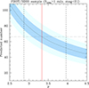 |
Fig. 2. Predicted number of z ≥ 4 QSOs (both blazars and non-blazars) with the flux density at 1.4 GHz ≥1 mJy and magdrop ≤ 21 in the sky area covered by the FIRST sample based on the observed number of blazars in the same area. The predictions are shown as a function of the parameter ‘p’, while the shaded area shows the Poissonian uncertainty on this number (dark blue = 1σ, light blue = 2σ). The horizontal dashed line indicates the observed number of sources, while the vertical lines report the best value of p (red solid line) together with the 2σ confidence interval (black short-dashed lines). |
Another way of applying Eq. (2) is to split the sample at different flux limits and predict the expected number of jetted sources at each flux density. In this way, we do not just compare the total predicted number of sources with the observed one, but we also test the distribution of the numbers as a function of the flux limit. In addition, if we are confident that no, or very few, blazars with magdrop ≤ 21 are present at flux densities below the FIRST limit, we can even extrapolate this computation to lower fluxes since the presence of blazars at high flux densities implies the existence of well-defined numbers of misaligned objects at much lower flux densities. This is shown in Fig. 3, where we assumed the best-fit value of p = 3.3. Also in this figure, we quantified the impact of the sources without a classification as blazar or non-blazar by assuming the extreme scenario in which all the unclassified sources with a radio loudness above 80 are blazars; this corresponds to the upper part of the light-blue area reported in the figure. Realistically, the correct curve should fall within the blue-shaded area, probably closer to the lowest line (corresponding to the case where no blazars are present among the unclassified objects). We also evaluated the impact of the blazar classifications that are not confirmed by VLBI data (see Appendix B) by excluding them from the analysis (dashed line) and assuming p = 3.0. As is clear from the figure, the impact of the possible misclassifications is marginal.
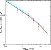 |
Fig. 3. Predicted number on a sky area of 10 000 sq. degrees of z ≥ 4 jetted type 1 QSOs (blazars+misaligned sources) with magdrop ≤ 21 for different radio flux density limits based on the high-z blazars currently detected at 1.4 GHz in the FIRST sample (mostly at flux densities above 10 mJy) described in the text. The predictions (black solid line) assume the best value of p (3.3). The light blue-shaded area indicates the possible impact of the sources with missing classification under the (extreme) assumption that all the sources missing X-ray data and with a radio loudness above 80 are blazars. The dashed line shows the impact of the misclassifications; the line was computed by excluding all blazars that have not been confirmed by VLBI observation (see Appendix B). In this case, we assume p = 3.0. The red points represent the observed sources from the FIRST catalogue, while the magenta point indicates the extension down to the 0.5 mJy beam−1 based on FIRST maps. |
Overall, the shape of the distribution seems in good agreement with the predictions, considering the statistical errors, although the last point at 0.5 mJy suggests a possible flattening of the curve. This hint of flattening, however, is statistically marginal, and it could be related to some incompleteness of our extension of the FIRST catalogue below 1 mJy. More data are required in order to confirm this possible trend.
In case of a significant deficit of sources observed at low flux densities compared to the predictions, it will be possible to infer the presence of an obscuring structure and to quantify its angular aperture. For instance, according to the AGN unified model, we expect that above a certain viewing angle the line of sight will intercept the molecular torus that will obscure the innermost QSO emission, such as that from the broad-line region (BLR) and the accretion disc. The consequence will be a progressive paucity of observed type 1 QSOs (the class of sources that we consider in this work) when moving towards lower radio flux densities, where sources are observed, on average, at larger angles.
If we take this effect into account, we would expect a flattening of the number of jetted (type 1) QSOs below a critical flux density that depends on the torus aperture. We note that while the number of jetted QSOs predicted according to Eq. (2) does not depend on the Lorentz factor, the flux density limit at which we expect the flattening does. Indeed, for a given torus critical aperture, the corresponding observed flux density depends on the jet bulk velocity. For larger (lower) values of Γ, the break on the number density would be observed at lower (larger) flux densities. In Fig. 4, we report the expected number of jetted type 1 QSOs at z ≥ 4 and magdrop ≤ 21 in a sky area of 10 000 sq. degrees at different flux density limits considering different torus apertures expressed in units of ‘blazar’ angle Θb = 1/Γ.
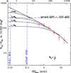 |
Fig. 4. Same as Fig. 3 but showing the impact of a circumnuclear obscuring torus with different aperture angles expressed in units of beaming angle Θb = 1/Γ (the uppermost line represents the case of no absorption). The upper scale of the figure shows the representative values of radio loudness (R) corresponding to the flux density limit in the X-axis and using a magnitude of 21 and assuming an average redshift of 4.5. The depth (5 × rms) of some ongoing and/or planned surveys is also indicated. The points are as in the previous figure. The horizontal dashed line indicates the expected total number of jetted QSOs in 10 000 sq. degrees if they represent 10% of the total QSO population. |
Assuming that there are no blazars among the unclassified sources, the data points currently do not suggest the presence of a significant level of obscuration at angles lower than approximately two times the critical angle Θb (i.e., below 10–20° for Γ = 10 − 5, respectively). The detection of some new blazars among the unclassified source may increase the discrepancy between the point at 0.5 mJy and the predictions, although, as explained above, this point may suffer from some incompleteness. Deeper radio surveys are necessary to better quantify the number of sources at flux densities below 1 mJy and to extend this test to even lower fluxes, which correspond to larger viewing angles (see Sect. 5).
4.3. Fraction of jetted quasi-stellar objects and absorption
Since we built the FIRST sample on a sky area where the total number of z ≥ 4 QSOs (both radio quiet and radio loud) with magdrop ≤ 21 is known, mostly thanks to the SDSS spectroscopic archive, it is possible to estimate the fraction of jetted QSOs at these redshifts. The LogN–LogS presented in Fig. 4 is expected to converge, at very low flux densities, to the total number of jetted QSOs, that is, 2Γ2 × Nblazar (see discussion in Sect. 2). Since we deal only with un-obscured sources, the actual number is
where fobsc is the fraction of obscured sources (Nobsc/Ntot). Therefore, the existence of 20 blazars in this area and with magdrop ≤ 21 implies the existence of ∼(1000 − 4000)×(1 − fobsc) jetted type 1 QSOs with the same optical limit, using Γ = 5 − 10, respectively. If we assume that the fraction of obscured (type 2) jetted QSOs is similar to that proposed for the total QSO population (∼70%, Vito et al. 2018), we expect, in this sky area, 300–1200 jetted type 1 QSOs, most of which are not detectable in the existing radio surveys due to their very low radio flux. In the same area of sky we have counted 1330 z ≥ 4 QSO, independently to the radio detection (see Sect. 4). Therefore, depending on the actual value of Γ, a significant fraction (23–90% for Γ = 5 and 10, respectively) of QSOs at z ≥ 4 could have a powerful relativistic jet currently not detected because it is strongly de-beamed. This result is consistent with what has been found by Diana et al. (2022) using blazars in the CLASS survey (see their Fig. 5), but it is in apparent disagreement (in particular for high Lorentz factors) with the results presented by Liu et al. (2020), who found a radio-loud fraction at z ∼ 6 close to 10% (9.4 ± 5.7%). We note, however, that a direct comparison of this number with the fraction of jetted QSOs derived above is difficult since our estimate of the fraction of jetted QSOs is not based on the value of radio loudness, as in Liu et al. (2020), who used R > 10 to define a QSO as radio loud. In our estimate, the misaligned jetted QSOs that we infer from the observed number of blazars do not necessarily have R > 10 since their core emission is expected to be significantly de-beamed at large viewing angles (see Sect. 5 for a discussion). And, indeed, seven objects in the FIRST sample have a radio-loudness between one and 10. In this sense, the definition of radio-loud QSO has a somewhat ambiguous meaning, particularly when the radio flux is dominated by the core emission, which is strongly dependent on orientation (see also the discussion in Sbarrato et al. 2021).
Alternatively, if we assume that the fraction of jetted QSOs is similar to what is found in Liu et al. (2020; ∼10%), the fraction of obscured sources must be much higher than 70%, on the order of 87%–97%. Therefore, assessing the importance of obscuration in high-z jetted QSOs is intimately related to the problem of how ubiquitous powerful relativistic jets were in the primordial Universe.
In order to distinguish between these scenarios (high fraction of jetted QSOs or high fraction of obscured QSOs), we needed to reach low flux densities. In Fig. 4, we show a case where jetted QSOs represent 10% of the total population (dashed horizontal line). This is the value to which the log N–log S should converge at low radio flux densities if the fraction of jetted QSOs is really 10%. Reaching flux densities of ∼0.1 mJy would already allow us to confirm or reject this possibility, and this is a feasible task that can be accomplished in the next few years, as discussed in the next section.
5. Predictions at sub millijansky flux densities
The next coming years will be particularly promising as far as radio surveys are concerned. Square Kilometre Array precursors and pathfinders, and subsequently the SKA Observatory (SKAO) itself, are carrying out, or have plans to carry out, several continuum surveys that will significantly improve the existing ones. From Fig. 4 it is clear that we need surveys covering a significant portion of the sky (at least a few thousands of square degrees in order to find a sizeable number of objects) and reaching flux density limits below 100 μJy beam−1, which is where we may expect to see a flattening of the high-z radio loud QSO number counts. A critical point when going to such a low flux density level is that the core emission may no longer be dominant because of the strong de-beaming expected at large viewing angles. The presence of a significant fraction of extended emission8 may cause the sample to include more sources than expected on the basis of the sole core emission, thus affecting the analysis. Using high frequencies may help limit this problem but will not completely eliminate it. Therefore, a good spatial resolution, of less than a few arcseconds, will also be very important to resolving the source and distinguishing the core from the extended emission.
At the ∼1 GHz frequency, a promising survey is the Evolutionary Map of the Universe (EMU), which is ongoing at the Australian SKA Pathfinder (ASKAP) radio telescope (Norris et al. 2011, 2021). The survey will cover the sky at declination below +30° and have an expected rms noise level of 20–25 μJy beam−1. Unfortunately, the resolution of EMU is relatively poor (∼12″), and the separating core and extended emission may not be always possible. A follow-up of the detected sources might be necessary in order to estimate the correct flux density from the core.
An outstanding improvement, both in sensitivity and angular resolution, will be possible thanks to the wide-field continuum surveys that will be carried out by SKA1-Mid. The continuum sensitivity (rms in 1 h) is expected to be 2 μJy beam−1 at 1.4 GHz, with a resolution of 0.4″ (Braun et al. 2019). With this kind of imaging sensitivity and resolution, it will be possible to robustly test for the presence of obscuration at large viewing angles.
In Fig. 4, we show the 5 × rms flux limit of the surveys mentioned above, revealing their actual capability of distinguishing between different scenarios. Reaching flux densities of a few tens of micro-Jansky should allow us to test for the presence of obscuration at angles up to ∼30–35°, where the ‘standard’ obscuring torus should be present.
An important point that should be considered when moving towards such low radio flux densities while keeping the same optical limit is that, at a certain flux level, we start sampling the population of QSOs whose radio emission is not powered by a relativistic jet but could be related, for instance, to an intense star formation. These are the sources usually classified as ‘radio-quiet’ on the basis of a low radio loudness (R < 1). While the presence of a relativistic jet is well established in radio loud QSOs with a radio loudness above 10, in radio-quiet QSOs, the origin of the radio emission is still a matter of debate. In the top axis of Fig. 4, we report the values of radio-loudness computed using the radio flux density limit on the X-axis and the optical flux density at 4400 Å corresponding to magdrop = 21 and assuming z = 4.5, αR = 0.19, and αO = 0.44 (Vanden Berk et al. 2001). This scale gives an approximate indication of the typical values of R expected at each radio flux limit. For instance, among the 73 sources in the FIRST sample we discussed, the majority (65) have R > 10 in the typical range of radio loud QSO, and the remaining having R between 1 and 10. In the deeper ongoing or planned surveys, such as ASKAP-EMU, we would instead expect a significant fraction of sources with R between 1 and 10 or even below 1. The sample based on the very deep SKA1-Mid surveys will be almost completely made up by objects with a value of R in the radio-quiet range (< 1). This is interesting since the simple discovery of high-z blazars at high flux densities (> 10 mJy) implies the existence of many misaligned jetted high-z QSOs well in the ‘radio-quiet regime’ (the actual number depends on the importance of the extended emission, as explained above). Recent results by Sbarrato et al. (2021) suggest that some high-z QSOs with a radio loudness well below the radio loud-radio quiet threshold do actually show evidence for the presence of a misaligned jet, putting into question the simple use of the radio loudness parameter to discriminate between jetted and non-jetted QSOs, at least in this range of redshift.
In any case, the overlap between the misaligned jetted QSOs and the non-jetted QSOs, whose radio emission could be due to star formation or other mechanisms, is a potential issue since the possible inclusion of non-jetted QSOs in the plot shown in Fig. 4 is expected to produce a steepening of the curve below a certain flux limit, thus affecting the final results. In principle, it should be possible to distinguish between the two classes of sources by studying the radio morphology (at arcsec and sub-arcsecond scales), as demonstrated by Sbarrato et al. (2021), or using the value of brightness temperature measured in high resolution radio images (see e.g., Morabito et al. 2022). In this context, wide-field VLBI surveys would be ideal to assess the presence of a jet (e.g., Radcliffe et al. 2021). Also, the observed radio luminosity can be used to distinguish QSOs whose radio emission is powered by a jet from those whose emission is powered by star formation. For example, all the sources in the FIRST sample with a radio loudness parameter between 1 and 10 have radio powers at 1.4 GHz between 1026 and 1027 W Hz−1, that is, well within the typical range of the power observed in jetted QSOs, despite their relatively low radio loudness values.
6. Conclusions
We have discussed and further developed a method first proposed by Ghisellini & Sbarrato (2016) to evaluate the presence of obscuration in jetted QSOs in the early Universe (z ≥ 4) based on the number of blazars observed in a flux-limited sample. We applied this method to two well-defined samples of high-z type 1 jetted QSOs containing, in total, 87 independent z ≥ 4 radio-emitting QSOs, including 31 sources classified as blazars on the basis of their X-ray emission.
The first sample, the CLASS high-z sample, contains 23 sources and is characterised by a high radio flux density limit (30 mJy at 5 GHz). The second sample is based on a combination of the last data release of SDSS (DR17) and FIRST, and it contains 73 sources (with nine sources in common with the CLASS sample). This sample has a much deeper radio limit (0.5 mJy) compared to CLASS, but it has the same optical limit (magdrop = 21). The main results of our work can be summarised as follows:
-
In the CLASS sample, blazars represent a large majority (∼85%) of the sources, with only a small fraction of misaligned objects. Our analysis showed that this dominance of oriented sources is consistent with the predictions of the beaming model, and therefore, it is likely due to the high radio-to-optical flux limit ratio of the CLASS sample that favours the selection of oriented sources, and it is not caused by the obscuration along large lines of sight.
-
When using the FIRST sample, which contains a larger fraction of misaligned sources compared to CLASS, we did not observe any significant departure from the beaming model predictions, although there is a hint of a possible deviation at low flux densities (∼0.5 mJy). It is possible, however, that this suggested trend is simply due to the incompleteness of the FIRST survey at this low flux density limit.
-
Since a reliable blazar–non-blazar classification based on X-ray data is only present for the radio brightest sources in the FIRST sample (i.e., for ∼40% of the objects), we cannot exclude that a discrepancy may appear once all the sources in the sample are correctly classified. However, considering that only sources with a relatively high radio loudness are reasonable blazar candidates, the impact of the unclassified sources is quite marginal. Swift-XRT observations of the objects in the sample with the highest radio loudness are in progress. In addition, the first data release of the eROSITA All Sky Survey (Merloni et al. 2012), expected within the next months, will certainly help classify the sources since even a non-detection can be used to exclude their blazar nature.
-
Next generation radio surveys, such as ASKAP EMU and eventually those carried out with SKA1-Mid, will be able to sample much deeper radio limits and therefore much larger observing angles compared to the existing surveys. At some point, we do expect to observe a significant departure from the predictions due to the presence of the ‘standard’ obscuring torus. At these very low flux densities (tens of micro-Jansky), however, distinguishing between misaligned QSOs and radio-quiet QSOs, that is, sources not powered by a radio jet, could be challenging, as the radio loudness parameter is expected to no longer be useful in separating the two types of sources. High-resolution radio follow-up will be instrumental to distinguishing the two classes of AGN. Another critical point will be separating the core emission from that coming from isotropic extended structures since at large observing angles, the former will become less relevant. Again, using data with a good resolution and at the highest possible frequency will be fundamental for a reliable analysis.
Assessing the fraction of optically absorbed jetted high-z QSOs is also fundamental to establishing how common powerful relativistic jets were in the early Universe. If the fraction of optically absorbed sources is similar to that estimated in high-z radio-quiet QSOs (∼70%), the number of jetted QSOs could be much higher compared to the local Universe, representing up to 90% of the QSO population. Conversely, if jetted QSOs represent only ∼10% of the total population, as in the local Universe, the fraction of obscured jetted QSOs could be much higher than expected, between 87% and 97%. Deep radio surveys will be instrumental to distinguishing between these two possible (and intriguing) scenarios.
The solid angle corresponding to Θb is 2π(1-cosΘb). Since jets are emitted along two opposite directions, Ωb is two times this value, that is, Ωb = 4π(1 − cosΘb)∼2π/Γ2 (valid for small angles).
We note that in Ghisellini & Sbarrato (2016), this number is wrongly given as the ratio between Ntot and the number of blazars (their Eq. (8)).
These objects are the only known z > 4 QSOs in the sky area covered by CLASS with a flux density at 5 GHz above 30 mJy. In principle, there could be more sources not yet discovered as high-z QSOs. However, most of the high-z QSOs in the northern sky and with mag ≤ 21 should have already been found, thanks to the Sloan Digital Sky Survey (SDSS) spectral database (see also discussion in Sect. 4).
According to Ighina et al. (2019), we define  , where L10 keV and L2500 Å are, respectively, the X-ray and UV monochromatic luminosities (per unit of frequency). Blazars are characterised by
  .
.
It is, however, possible that extended emission in the early Universe was strongly dumped due to the interaction with the CMB, as mentioned in Sect. 2.
We note that αR = 0.1 is the average spectral slope measured for the sources in the sample between 144/150 MHz and 1.4 GHz using data from LoTSS (Shimwell et al. 2022) and TGSS (Intema et al. 2017). These indices are reported in Table C.1.
We used different flux distributions. We started with luminosity functions with different slopes, but we found that the result does not depend on the assumed function.
The Doppler factor is defined as δ = [Γ(1 − βcosθ)]−1, where Γ and β are the Lorentz factor and the ratio between the bulk velocity and the light speed, respectively.
Acknowledgments
We acknowledge financial contribution from the agreement ASI-INAF n. I/037/12/0 and n. 2017-14-H.0 and from INAF under PRIN SKA/CTA FORECaST. We acknowledge financial support from INAF under the project ‘QSO jets in the early Universe’, Ricerca Fondamentale 2022 and under the project ‘Testing the obscuration in the Early Universe’, Ricerca Fondamentale 2023. C.S. acknowledges financial support from INAF (Grants 1.05.12.04.04). This work has been partially supported by the ASI-INAF program I/004/11/4. This work is based on FIRST and SDSS data. Funding for the Sloan Digital Sky Survey V has been provided by the Alfred P. Sloan Foundation, the Heising-Simons Foundation, the National Science Foundation, and the Participating Institutions. SDSS acknowledges support and resources from the Center for High-Performance Computing at the University of Utah. The SDSS web site is www.sdss.org.
References
- Aird, J., Coil, A. L., Georgakakis, A., et al. 2015, MNRAS, 451, 1892 [Google Scholar]
- Antonucci, R. 1993, ARA&A, 31, 473 [Google Scholar]
- Bañados, E., Venemans, B. P., Morganson, E., et al. 2015, ApJ, 804, 118 [Google Scholar]
- Bañados, E., Venemans, B. P., Decarli, R., et al. 2016, ApJS, 227, 11 [Google Scholar]
- Bañados, E., Mazzucchelli, C., Momjian, E., et al. 2021, ApJ, 909, 80 [CrossRef] [Google Scholar]
- Bañados, E., Schindler, J.-T., Venemans, B. P., et al. 2022, ApJS, 265, 29 [Google Scholar]
- Becker, R. H., White, R. L., & Helfand, D. J. 1995, ApJ, 450, 559 [Google Scholar]
- Belladitta, S., Moretti, A., Caccianiga, A., et al. 2023, A&A, 669, A134 [NASA ADS] [CrossRef] [EDP Sciences] [Google Scholar]
- Braun, R., Bonaldi, A., Bourke, T., Keane, E., & Wagg, J. 2019, arXiv e-prints [arXiv:1912.12699] [Google Scholar]
- Caccianiga, A., Moretti, A., Belladitta, S., et al. 2019, MNRAS, 484, 204 [NASA ADS] [CrossRef] [Google Scholar]
- Cao, H. M., Frey, S., Gabányi, K. É., et al. 2017, MNRAS, 467, 950 [Google Scholar]
- Chambers, K. C., Magnier, E. A., Metcalfe, N., et al. 2016, arXiv e-prints [arXiv:1612.05560] [Google Scholar]
- Coppejans, R., Frey, S., Cseh, D., et al. 2016, MNRAS, 463, 3260 [Google Scholar]
- Diana, A., Caccianiga, A., Ighina, L., et al. 2022, MNRAS, 5447, 5436 [CrossRef] [Google Scholar]
- Drlica-Wagner, A., Carlin, J. L., Nidever, D. L., et al. 2021, ApJS, 256, 2 [NASA ADS] [CrossRef] [Google Scholar]
- Drlica-Wagner, A., Ferguson, P. S., Adamów, M., et al. 2022, ApJS, 261, 38 [NASA ADS] [CrossRef] [Google Scholar]
- Drouart, G., Seymour, N., Galvin, T. J., et al. 2020, PASA, 37, 26 [NASA ADS] [CrossRef] [Google Scholar]
- Endsley, R., Stark, D. P., Fan, X., et al. 2022, MNRAS, 4261, 4248 [CrossRef] [Google Scholar]
- Evans, I. N., Primini, F. A., Glotfelty, K. J., et al. 2010, ApJS, 189, 37 [NASA ADS] [CrossRef] [Google Scholar]
- Evans, P. A., Page, K. L., Osborne, J. P., et al. 2020, ApJS, 247, 54 [Google Scholar]
- Fan, X., Banados, E., & Simcoe, R. A. 2022, ARA&A, 61, 373 [Google Scholar]
- Frey, S., Gurvits, L. I., Paragi, Z., & Gabányi, K. É. 2008, A&A, 484, L39 [NASA ADS] [CrossRef] [EDP Sciences] [Google Scholar]
- Frey, S., Paragi, Z., Gurvits, L. I., Cseh, D., & Gabanyi, K. E. 2010, A&A, 524, A83 [NASA ADS] [CrossRef] [EDP Sciences] [Google Scholar]
- Frey, S., Paragi, Z., Gurvits, L. I., Gabányi, K. É., & Cseh, D. 2011, A&A, 531, L5 [NASA ADS] [CrossRef] [EDP Sciences] [Google Scholar]
- Frey, S., Titov, O., Melnikov, A. E., de Vicente, P., & Shu, F. 2018, A&A, 618, A68 [NASA ADS] [CrossRef] [EDP Sciences] [Google Scholar]
- Gabanyi, K. E., Cseh, D., Frey, S., et al. 2015, MNRAS, 450, 57 [Google Scholar]
- Ghisellini, G., & Sbarrato, T. 2016, MNRAS, 461, L21 [NASA ADS] [CrossRef] [Google Scholar]
- Ghisellini, G., & Tavecchio, F. 2009, MNRAS, 397, 985 [Google Scholar]
- Ghisellini, G., Della Ceca, R., Volonteri, M., et al. 2010, MNRAS, 405, 387 [NASA ADS] [Google Scholar]
- Ghisellini, G., Sbarrato, T., Tagliaferri, G., et al. 2014, MNRAS, 440, 111 [Google Scholar]
- Ghisellini, G., Perri, M., Costamante, L., et al. 2019, A&A, 627, A72 [NASA ADS] [CrossRef] [EDP Sciences] [Google Scholar]
- Gilli, R., Norman, C., Calura, F., et al. 2022, A&A, 666, A17 [NASA ADS] [CrossRef] [EDP Sciences] [Google Scholar]
- Gloudemans, A. J., Duncan, K. J., Saxena, A., et al. 2022, A&A, 668, A27 [NASA ADS] [CrossRef] [EDP Sciences] [Google Scholar]
- Gregory, P. C., Scott, W. K., Douglas, K., & Condon, J. J. 1996, ApJS, 103, 427 [NASA ADS] [CrossRef] [Google Scholar]
- Heckman, T. M., & Best, P. N. 2014, ARA&A, 52, 75 [Google Scholar]
- Hurley-Walker, N., Galvin, T. J., Duchesne, S. W., et al. 2022, PASA, 39, e035 [NASA ADS] [CrossRef] [Google Scholar]
- Ighina, L., Caccianiga, A., Moretti, A., et al. 2019, MNRAS, 489, 2732 [NASA ADS] [CrossRef] [Google Scholar]
- Ighina, L., Caccianiga, A., Moretti, A., et al. 2021, MNRAS, 505, 4120 [NASA ADS] [CrossRef] [Google Scholar]
- Intema, H. T., Jagannathan, P., Mooley, K. P., & Frail, D. A. 2017, A&A, 598, A78 [NASA ADS] [CrossRef] [EDP Sciences] [Google Scholar]
- Kellermann, K. I., Sramek, R., Schmidt, M., Shaffer, D. B., & Green, R. 1989, AJ, 98, 1195 [Google Scholar]
- Koptelova, E., & Hwang, C.-Y. 2022, ApJ, 929, L7 [NASA ADS] [CrossRef] [Google Scholar]
- Krezinger, M., Perger, K., Gabányi, K. É., et al. 2022, ApJS, 260, 49 [NASA ADS] [CrossRef] [Google Scholar]
- Lister, M. L., Homan, D. C., Hovatta, T., et al. 2019, ApJ, 874, 43 [NASA ADS] [CrossRef] [Google Scholar]
- Liu, Y., Wang, R., Momjian, E., et al. 2020, ApJ, 256, 2 [Google Scholar]
- Liu, Y., Wang, R., Momjian, E., et al. 2022, ApJ, 939, 5 [Google Scholar]
- Mainzer, A., Bauer, J., Cutri, R. M., et al. 2014, ApJ, 792, 30 [Google Scholar]
- Merloni, A. 2016, Astrophysical Black Holes (Switzerland: Springer International Publishing), Lect. Notes Phys., 905, 101 [NASA ADS] [CrossRef] [Google Scholar]
- Merloni, A., Predehl, P., Becker, W., et al. 2012, arXiv e-prints [arXiv:1209.3114] [Google Scholar]
- Merloni, A., Bongiorno, A., Brusa, M., et al. 2014, MNRAS, 437, 3550 [Google Scholar]
- Momjian, E., Bañados, E., Carilli, C. L., Walter, F., & Mazzucchelli, C. 2021, AJ, 161, 207 [NASA ADS] [CrossRef] [Google Scholar]
- Morabito, L. K., Sweijen, F., Radcliffe, J. F., et al. 2022, MNRAS, 515, 5758 [NASA ADS] [CrossRef] [Google Scholar]
- Moretti, A., Vattakunnel, S., Tozzi, P., et al. 2012, A&A, 548, A87 [NASA ADS] [CrossRef] [EDP Sciences] [Google Scholar]
- Netzer, H. 2015, ARA&A, 53, 653 [Google Scholar]
- Norris, R. P., Hopkins, A. M., Afonso, J., et al. 2011, PASA, 28, 215 [Google Scholar]
- Norris, R. P., Marvil, J., Collier, J. D., et al. 2021, PASA, 38, 46 [NASA ADS] [Google Scholar]
- Pacucci, F., & Loeb, A. 2021, MNRAS, 509, 1885 [NASA ADS] [CrossRef] [Google Scholar]
- Paliya, V. S., Ajello, M., Cao, H. M., et al. 2020, ApJ, 897, 177 [NASA ADS] [CrossRef] [Google Scholar]
- Radcliffe, J. F., Barthel, P. D., Thomson, A. P., et al. 2021, A&A, 649, A27 [EDP Sciences] [Google Scholar]
- Sbarrato, T., Ghisellini, G., Nardini, M., et al. 2012, MNRAS, 426, L91 [Google Scholar]
- Sbarrato, T., Ghisellini, G., Nardini, M., et al. 2013a, MNRAS, 433, 2182 [NASA ADS] [CrossRef] [Google Scholar]
- Sbarrato, T., Tagliaferri, G., Ghisellini, G., et al. 2013b, ApJ, 777, 147 [Google Scholar]
- Sbarrato, T., Ghisellini, G., Tagliaferri, G., et al. 2015, MNRAS, 446, 2483 [NASA ADS] [CrossRef] [Google Scholar]
- Sbarrato, T., Ghisellini, G., Giovannini, G., & Giroletti, M. 2021, A&A, 655, A95 [NASA ADS] [CrossRef] [EDP Sciences] [Google Scholar]
- Sbarrato, T., Ghisellini, G., Tagliaferri, G., et al. 2022, A&A, 663, A147 [NASA ADS] [CrossRef] [EDP Sciences] [Google Scholar]
- Schindler, J.-T., Fan, X., McGreer, I. D., et al. 2017, ApJ, 851, 13 [NASA ADS] [CrossRef] [Google Scholar]
- Shimwell, T. W., Hardcastle, M. J., Tasse, C., et al. 2022, A&A, 659, A1 [NASA ADS] [CrossRef] [EDP Sciences] [Google Scholar]
- Spingola, C., Dallacasa, D., Belladitta, S., et al. 2020, A&A, 643, L12 [EDP Sciences] [Google Scholar]
- Stern, D., Djorgovski, S. G., Perley, R. A., de Carvalho, R. R., & Wall, J. V. 2000, AJ, 119, 1526 [Google Scholar]
- Tadhunter, C. 2016, A&ARv, 24, 10 [Google Scholar]
- Urry, C. M., & Padovani, P. 1995, PASP, 107, 803 [NASA ADS] [CrossRef] [Google Scholar]
- Vanden Berk, D. E., Richards, G. T., Bauer, A., et al. 2001, AJ, 122, 549 [Google Scholar]
- Vijarnwannaluk, B., Akiyama, M., Schramm, M., et al. 2022, ApJ, 941, 97 [NASA ADS] [CrossRef] [Google Scholar]
- Vito, F., Brandt, W. N., Yang, G., et al. 2018, MNRAS, 473, 2378 [Google Scholar]
- Wayth, R. B., Tingay, S. J., Trott, C. M., et al. 2018, PASA, 35, 33 [Google Scholar]
- Wu, J., Brandt, W. N., Miller, B. P., et al. 2013, ApJ, 763, 109 [NASA ADS] [CrossRef] [Google Scholar]
- Yang, G., Caputi, K. I., Papovich, C., et al. 2023, ApJ, 950, L5 [NASA ADS] [CrossRef] [Google Scholar]
- Zeimann, G. R., White, R. L., Becker, R. H., et al. 2011, ApJ, 736, 57 [Google Scholar]
- Zhang, Y., An, T., Yang, X., et al. 2021, MNRAS, 507, 3736 [NASA ADS] [CrossRef] [Google Scholar]
Appendix A: Blazars and non-blazars in a flux-limited sample
We tested the method presented by Ghisellini et al. (2019) and discussed in Sect. 2 (equation 1) using numerical simulations. Equation 1 gives the total number of jetted QSOs expected in a flux-limited sample given the flux densities of all the blazars discovered in the same sample. To test this formula, we started from a population of un-beamed sources with an intrinsic (i.e. rest frame) flux density ranging from 0.01 mJy to 100 mJy10 and randomly associated a viewing angle with each source. We then applied the beaming factor to these sources, assuming different values of Γ (5, 10, and 15) and p (2 and 3), and we considered only the sources above a certain flux limit (we used 30 mJy, which is the limit of the CLASS sample, but the results can be re-scaled to any value). We then classified as blazars all the sources with θ < 1/Γ and applied equation 1 to recover the expected number of sources, both blazars and misaligned objects, above the flux limit. This value was then compared to the actual number of objects above the same limit.
We note that in these simulations we have assumed that there is no extended un-beamed emission, and therefore, we expected that the value of Ntot provided by equation 1 should match exactly with the actual value of the sources given as input. In real data, extended emission may give a contribution, although as discussed in Sect. 2, we do not expect that this is relevant for the samples studied in this work.
Depending on the assumed values of the intrinsic flux density Γ and p, we obtained different values of the total-to-blazar number ratio. Figure A.1 shows the results of the comparison between the predicted ratio derived from equation 1 and the real one. It appears that equation 1 systematically overestimates (by a factor ∼1.4) the true total number of sources in the sample (blue lines). The overestimation is nearly independent of the assumed value of the input parameters.
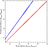 |
Fig. A.1. Results of a simulation where N jets of equal radio flux density have been randomly oriented on the sky and relativistically beamed according to the angle (θ) between the jet and the observer. We assumed different values of the beaming parameters (i.e. Γ = 5, 10, 15 and p = 2 and 3) and different starting values of the un-beamed radio flux density (from 0.01 to 100 mJy). We then imposed a flux limit of 30 mJy and classified all the sources with θ < 1/Γ as blazars. These combinations yielded different values (from 1 to 10) for the ratio between the total number of sources (blazar+misaligned objects) and blazars that are included in the simulated sample. Finally, we applied Eq 1 and Eq 2 to the simulated blazar sample (assuming the correct value of p) to recover the expected total number of sources above the flux limit. In the figure, we compare the predicted total-blazar number ratio with the true one. Equation 1 (blue line) systematically overestimates the result by a factor of ∼1.4, while equation 2 (red line) provides the correct results. |
The origin of this discrepancy is likely related to the fact that equation 1 was derived by assuming that all the blazars in the sample are oriented exactly at an angle equal to 1/Γ. At this angle, the Doppler factor11 is equal to Γ. This is clearly an approximation since the actual viewing angles of a sample of blazars are expected to be distributed between 0° and 1/Γ. A more correct number should be given by the average value of the Doppler factor computed with all the sources observed within 1/Γ. This average value is expected to be larger than Γ. The average Doppler factor for a sample of blazars is given by
 (A.1)
(A.1)
By including this correction in the derivation of equation 1 presented in Ghisellini & Sbarrato (2016), we obtain
![Mathematical equation: $$ \begin{aligned} N_{tot} \sim \sum _{i=1}^N {[1.44(\frac{S_i}{S_{lim}})^{1/p} -1]}. \end{aligned} $$](/articles/aa/full_html/2024/04/aa48561-23/aa48561-23-eq16.gif) (A.2)
(A.2)
Again, we tested this relation through our numerical simulations (red line in Fig A.1), and we found that it correctly recovers the true total number of sources.
Appendix B: Reliability of the classifications
As mentioned in Sect. 4.1, the classification of a source as blazar is not straightforward, and it may depend on the method one has adopted. Recently, Krezinger et al. (2022) pointed out some discrepancies between classification based on SED analysis and another based on VLBI data. Among the high-z QSOs in the samples considered in this work, there are 16 objects with a classification from the literature based on VLBI data. While the two classifications agree in most (70%) cases, there seems to be a disagreement in five cases. These cases are discussed below.
J083946.2+511202. This source is classified as blazar based on the  (=1.25). The blazar nature is also suggested by analysis of the SED (Sbarrato et al. 2013a). Quite consistently to this classification, VLBI data (Cao et al. 2017) show a flat-spectrum, variable, and quite compact core. However, the Tb estimated from the deconvolved size (3.0±0.5×10¹⁰ K) is close but below the equipartition limit. This is likely a borderline source (also from the
  point of view) whose exact orientation could be near the one expected for blazars.
J103717.7+182303. The value of  of this object is similar to the one computed for the previous source (1.28) and is suggestive of a blazar nature. From analysis of the SED, Sbarrato et al. (2022) concluded that this source is either a blazar or a source viewed at the border of the definition. Again, VLBI data seem to resolve the emission, finding a relatively low value of Tb (2.6±0.5×10⁹ K), which is below the equipartition limit (Krezinger et al. 2022). As for J083946.2+511202, this could be a source at the border of the blazar definition.
J114657.8+403708. This object is classified as blazar on the basis of the X-ray data ( = 1.31) and of SED (Ghisellini et al. 2014). However, the value of Tb derived from the VLBI data (4.5±0.3×10⁹ K) is below the equipartition limit (Frey et al. 2010).
J123142.1+381659. The value of  computed for this object (1.18) indicates a blazar nature. The same classification is reported in Sbarrato et al. (2022), while Krezinger et al. (2022) suggested that the source is misaligned on the basis of the relatively low Tb (1.36±0.27×10⁹ K).
J142048.0+120546. We classified this source as blazar due to its low  (1.21), and this classification is supported by analysis of the SED (Sbarrato et al. 2015). The VLBI observations with EVN reveal a double morphology on a scale of 1.33″, which is too compact to be detected by FIRST data (Cao et al. 2017). Out of the two detected radio components, the most compact and brightest one is positionally coincident with the QSO, and it has Tb = 4.0±1.0×10⁹ K, which is high but still below the equipartition limit.
To summarise, all five cases of inconsistent classification between the two methods are quite similar, and they include sources with values of  below but close to the limit of 1.355 (typically 1.2-1.3) and show brightness temperatures that are relatively high (above 109K) but below the equipartition limit (0.3-5×10¹⁰ K). At the same time, we have four other sources with similar values of
  (∼1.2-1.3) but for which the VLBI observations confirm the presence of boosting. The remaining seven objects with VLBI data, that is, sources either with a very low value of
  (between 0.8 and 1.1, 4 objects) or a value above 1.355 (classified as non-blazars, three objects) have a consistent classification from VLBI data.
We conclude that the two methods are in reasonably good agreement, except for sources that are borderline ( between 1.2 and 1.3). In this range, ∼50% of the sources have a VLBI classification that seems to contradict the one inferred from the X-ray data. As already stated, these are cases that require a more careful analysis that takes into account all the possible pieces of information available. We also stress that the VLBI classification can be uncertain when the measured extensions, which are critical to determining the value of Tb, are only fractions of the synthesised beam and when the flux densities are relatively low compared to the local RMS. Only a synergic use of all the available multiwavelength data can provide the best possible classification. In any case, as discussed in Sect. 4.2, if we do not consider the sources with a controversial classification as blazars, the results presented in this paper do not change significantly.
Appendix C: The samples
In Tab C.1 we present the complete list of sources used in this paper. For each source in the CLASS and FIRST samples, we give the following quantities: Column 1 shows the name based on the optical coordinates. Columns 2 to 3 give the optical position. Column 4 provides the redshift derived from Caccianiga et al. (2019) or from SDSS except for four objects: 1Bañados et al. (2015), 2Gloudemans et al. (2022), 3Bañados et al. (2021), and 4Stern et al. (2000). Column 5 shows the magdrop corrected for Galactic reddening. The filter is specified between parentheses. Magnitudes are taken from the Pan-STARRS1 survey (PS1; Chambers et al. 2016) or from the DECam Local Volume Exploration Survey (DELVE; Drlica-Wagner et al. 2021; 2022). Column 6 provides the 1.4 GHz peak flux density from FIRST. Column 7 presents the 5 GHz flux density from the GB6 catalogue (Gregory et al. 1996). Column 8 shows the non-simultaneous radio spectral index (Sν ∝ ν−α) from 1.4 GHz and 144/150 MHz using FIRST and LoTSS (Shimwell et al. 2022) or TGSS (Intema et al. 2017) integrated flux densities. Column 9 indicates the sample: F=FIRST sample, C=CLASS sample. Column 10 shows the log of radio loudness computed using 1.4 GHz flux density and assuming the radio slope given in column 8 or assuming αr = 0.1 and using the near-infrared magnitude at 3.4 micron (W1) from the Wide-field Infrared Survey Explorer (NEOWISE; Mainzer et al. 2014), which provides the photometric point closest to the 4400Å rest-frame wavelength for z≥4 sources. To obtain the monochromatic flux at 4400Å we used the spectral index computed between W1 and the z-filter (or y-filter for z> 6.3 sources). If W1 was not available, we computed R using the z magnitude and assuming α0 = 0.44 (Vanden Berk et al. 2001). Column 11 presents the two-points-spectral index from radio to X-rays ( ). This was either taken from Ighina et al. (2019), for the sources in the CLASS sample, or computed using the available X-ray fluxes and the magnitudes in the z-filter. As for the radio loudness parameter, we used the optical spectral index computed between W1 and the z-filter, if available, or we assumed α0 = 0.44. The error on this parameter is mostly due to the uncertainty on the optical or UV slope and on the X-ray fluxes. Considering the range of values of slopes reported in Table 5 of Vanden Berk et al. (2001) (0.33-0.93) and the typical errors on the X-ray fluxes, we derived a typical error on
  of -0.03, +0.06. Column 12 shows the classification based on X-ray data: b=blazar (
 1.355), nb=non-blazar (
 ).
).
Sample of high-z jetted QSOs.
All Tables
All Figures
|
Fig. 1. Radio maps at 1.4 GHz from FIRST data of the seven high-z QSOs in the sample with peak flux densities between 0.5 and 0.9 mJy beam−1. These sources are not included in the FIRST catalogue. The levels were computed as −2, 2, 2.8, 4, 5.5, 8, ...times the rms (0.15 mJy beam−1). The central cross indicates the optical position of the high-z QSOs, while the beam size is reported in the bottom-left corner. |
| In the text | |
|
Fig. 2. Predicted number of z ≥ 4 QSOs (both blazars and non-blazars) with the flux density at 1.4 GHz ≥1 mJy and magdrop ≤ 21 in the sky area covered by the FIRST sample based on the observed number of blazars in the same area. The predictions are shown as a function of the parameter ‘p’, while the shaded area shows the Poissonian uncertainty on this number (dark blue = 1σ, light blue = 2σ). The horizontal dashed line indicates the observed number of sources, while the vertical lines report the best value of p (red solid line) together with the 2σ confidence interval (black short-dashed lines). |
| In the text | |
|
Fig. 3. Predicted number on a sky area of 10 000 sq. degrees of z ≥ 4 jetted type 1 QSOs (blazars+misaligned sources) with magdrop ≤ 21 for different radio flux density limits based on the high-z blazars currently detected at 1.4 GHz in the FIRST sample (mostly at flux densities above 10 mJy) described in the text. The predictions (black solid line) assume the best value of p (3.3). The light blue-shaded area indicates the possible impact of the sources with missing classification under the (extreme) assumption that all the sources missing X-ray data and with a radio loudness above 80 are blazars. The dashed line shows the impact of the misclassifications; the line was computed by excluding all blazars that have not been confirmed by VLBI observation (see Appendix B). In this case, we assume p = 3.0. The red points represent the observed sources from the FIRST catalogue, while the magenta point indicates the extension down to the 0.5 mJy beam−1 based on FIRST maps. |
| In the text | |
|
Fig. 4. Same as Fig. 3 but showing the impact of a circumnuclear obscuring torus with different aperture angles expressed in units of beaming angle Θb = 1/Γ (the uppermost line represents the case of no absorption). The upper scale of the figure shows the representative values of radio loudness (R) corresponding to the flux density limit in the X-axis and using a magnitude of 21 and assuming an average redshift of 4.5. The depth (5 × rms) of some ongoing and/or planned surveys is also indicated. The points are as in the previous figure. The horizontal dashed line indicates the expected total number of jetted QSOs in 10 000 sq. degrees if they represent 10% of the total QSO population. |
| In the text | |
|
Fig. A.1. Results of a simulation where N jets of equal radio flux density have been randomly oriented on the sky and relativistically beamed according to the angle (θ) between the jet and the observer. We assumed different values of the beaming parameters (i.e. Γ = 5, 10, 15 and p = 2 and 3) and different starting values of the un-beamed radio flux density (from 0.01 to 100 mJy). We then imposed a flux limit of 30 mJy and classified all the sources with θ < 1/Γ as blazars. These combinations yielded different values (from 1 to 10) for the ratio between the total number of sources (blazar+misaligned objects) and blazars that are included in the simulated sample. Finally, we applied Eq 1 and Eq 2 to the simulated blazar sample (assuming the correct value of p) to recover the expected total number of sources above the flux limit. In the figure, we compare the predicted total-blazar number ratio with the true one. Equation 1 (blue line) systematically overestimates the result by a factor of ∼1.4, while equation 2 (red line) provides the correct results. |
| In the text | |
Current usage metrics show cumulative count of Article Views (full-text article views including HTML views, PDF and ePub downloads, according to the available data) and Abstracts Views on Vision4Press platform.
Data correspond to usage on the plateform after 2015. The current usage metrics is available 48-96 hours after online publication and is updated daily on week days.
Initial download of the metrics may take a while.