| Issue |
A&A
Volume 684, April 2024
|
|
|---|---|---|
| Article Number | A5 | |
| Number of page(s) | 14 | |
| Section | Planets and planetary systems | |
| DOI | https://doi.org/10.1051/0004-6361/202348404 | |
| Published online | 28 March 2024 | |
Aligned fractures on asteroid Ryugu as an indicator of thermal fracturing
1
Institute for Planetary Research, German Aerospace Center (DLR), Rutherfordstraße 2, 12489 Berlin, Germany
e-mail: This email address is being protected from spambots. You need JavaScript enabled to view it.
; This email address is being protected from spambots. You need JavaScript enabled to view it.
2
Asteroid Engineering Laboratory, Lulea University of Technology, Kiruna, Sweden
e-mail: This email address is being protected from spambots. You need JavaScript enabled to view it.
3
Institut für Geologische Wissenschaften, Freie Universität Berlin, Malteserstraße 74-100, 12249 Berlin, Germany
4
Université Côte d’Azur, CNRS, Observatoire de la Côte d’Azur, Laboratoire Lagrange, Nice, France
5
Osaka University, Department of Earth and Space Science, Toyonaka, Japan
6
The University of Tokyo, Tokyo 113-0033, Japan
7
Planetary Exploration Research Center, Chiba Institute of Technology, Narashino 275-0016, Japan
Received:
27
October
2023
Accepted:
12
January
2024
Abstract
Context. Asteroid and comet surfaces are exposed to a complex environment that includes low gravity, high temperature gradients, and a bombardment of micrometeorites and cosmic rays. Surface material exposed to this environment evolves in a specific way depending on various factors such as the bodies’ size, heliocentric distance, and composition. Fractures in boulders, as seen on asteroid Ryugu, can help to determine and constrain the dominant processes eroding small-body surface materials. It is also possible to estimate fracture growth timescales based on the abundance and length of fractures in boulders.
Aims. We analyse the number, orientation, and length of fractures on asteroid Ryugu to establish the relation between the fractures and the processes that may have formed them. We also compare our results to similar investigations conducted on other small bodies and estimate the timescale of fracture growth.
Methods. 198 high-resolution Hayabusa2 images of asteroid Ryugu suitable for our fracture analysis were selected and map-projected. Within these images, fractures in boulders were manually mapped using the QGIS software. The fracture coordinates were extracted and the fractures’ orientation and length were computed for 1521 identified fractures.
Results. Fractures in boulders on asteroid Ryugu are found to be preferentially north-south aligned, suggesting a formation through thermal erosion. Modeling the fracture length indicates a fracture growth timescale of 30 000 to 40 000 yr, slightly younger than ages found previously for asteroid Bennu. The errors in these ages, due to uncertainties about the thermophysical parameters used in this model, are substantial (−33 000 yr +250 000 yr). However, even with these large errors, the model suggests that thermal fracturing is a geologically fast process. These times are not too dissimilar to those quoted in the literature for Ryugu and Bennu, since similar thermophysical material parameters for Ryugu and Bennu seem likely.
Key words: minor planets, asteroids: general / minor planets, asteroids: individual: Ryugu / minor planets, asteroids:individual: Bennu
© The Authors 2024
 Open Access article, published by EDP Sciences, under the terms of the Creative Commons Attribution License (https://creativecommons.org/licenses/by/4.0), which permits unrestricted use, distribution, and reproduction in any medium, provided the original work is properly cited.
This article is published in open access under the Subscribe to Open model. This email address is being protected from spambots. You need JavaScript enabled to view it. to support open access publication.
1 Introduction
To acquire a better understanding of the environment and processes that form and shape asteroids and comparable airless bodies, studies have demonstrated and quantified the influence of the thermal environment on the development of asteroid landscapes (Delbo et al. 2014, 2022; Molaro et al. 2015, 2017, 2020; Sasaki et al. 2020, 2022). One area of research that has received more attention in recent years is thermal fracturing, which is the process of rocks cracking and breaking due to temperature changes induced by repeated exposure to the Sun during rotation (El Mir et al. 2019). On small bodies, like asteroids Bennu and Ryugu, thermal fracturing can occur when the surface experiences repeated changes in temperature, occurring when the asteroid rotates and its surface is exposed repeatedly to sunlight and shadow. Other nonthermal processes that induce fracturing are (micro-) impacts or tidal effects (Ballouz et al. 2020; Hörz et al. 2020). It’s important to mention here that the breaking down of a boulder is likely the result of an interplay between (micro-) impacts and thermal effects. Which of these is dominant is not entirely clear and depends on factors such as the heliocentric distance of the body, the material composition, and the rotation period. On the Moon, for example, impacts are dominant (Rüsch & Bickel 2023; Basilevsky et al. 2015).
Through laboratory experiments and numerical simulations, researchers have found that thermal fracturing can lead to the formation of various surface features on small bodies, including boulders, rocks, and fractures within them. Additional morphologic observations such as of rock surface textures may also hint that this process is active on small bodies (Otto et al. 2020; Libourel et al. 2020). The presence and distribution of morphologic features may provide clues about the thermal history of the asteroid, as well as its physical properties and structural characteristics (Delbo et al. 2014, 2022; Molaro et al. 2020), although recently Rüsch & Bickel (2023) have shown that a specific morphological feature cannot necessarily be traced to a specific erosion agent (such as thermal fracturing or (micro-) impacts).
All of the recent studies above point out that thermal fracturing is therefore a key process that shapes the surface of small bodies like Ryugu, and studying its effects can provide valuable insights into the geological history of this object and the physical processes that govern its evolution.
Recently, Delbo et al. (2022) provided comprehensive insights into the timescales of thermal rock fracturing by analyzing NASA’s OSIRIS-REx images of the near-Earth asteroid Bennu. Through the evaluation of fracture orientation and frequency distributions, they attribute the origin of fractures to thermal stress. Their analytical model suggests a rapid formation timescale of 104–105 yr, a temporal frame with significant implications for asteroid evolution and material characteristics. This is corroborated by characteristic timescales of mass movement on Bennu, as is reported by Jawin et al. (2020).
In this study, we further substantiate Delbo et al. (2022) findings by extending their methodology to a second near-Earth asteroid, (162173) Ryugu. By applying their fracture analysis approach, we derive a fracture distribution and orientation for Ryugu’s surface.
Similar to Bennu, Ryugu is a near-Earth rubble-pile asteroid with a spinning top shape and a diameter of about 900 m (Watanabe et al. 2019), compared to Bennu’s diameter of 492 m. Ryugu’s rotation period (7.63 h) is almost double that of Bennu’s (4.30 h). Ryugu, designated as a C-type (carbonaceous) asteroid, exhibits a mineralogical, bulk chemical, and isotopic composition very similar to that of CI chondrites (Yada et al. 2021; Nakamura et al. 2023; Yokoyama et al. 2023). Bennu’s composition is not fully known at the time of writing, but a composition of CI and CM chondrites is likely (Hamilton et al. 2019). The thermal inertiae of Ryugu and Bennu are very similar (Okada et al. 2016; Grott et al. 2019; Sakatani et al. 2021; DellaGiustina et al. 2019; Rozitis et al. 2020; Cambioni et al. 2021), which is important for thermal modeling. Ryugu’s surface has a high abundance of boulders, ranging in diameter from 1 to 139 m (Wada et al. 2018; Michikami et al. 2019). “Boulders” of these sizes encompass superblocks, megablocks, blocks, and boulders according to the proposed nomenclature by Bruno & Ruban (2017), but since most of the observed clasts here are on the smaller side, the term “boulder” is used in this study. The cumulative size distribution of Ryugu’s boulders follows a power law with an exponent of −2.65, according to Michikami et al. (2019). The boulders have been classified earlier into three major categories, with a correlation between brightness and morphology: dark and rugged boulders, bright and smooth boulders, and bright and mottled boulders (Sugita et al. 2019b). To date, however, no special attention has been paid to boulder morphology and its relationship to fractures.
Ryugu’s history is thought to be complex: it likely formed as a rubble-pile asteroid from the debris of a much larger (approx. 100 km diameter) parent body that was fragmented by a catastrophic collision (Sugita et al. 2019b). It is possible that there were multiple stages of collisions and that two or more parent bodies broke apart and provided material to build Ryugu. Because of this Ryugu likely incorporated different lithologies of the original parent bodies (Sugita et al. 2019b).
The Hayabusa2 mission was launched on December 3, 2015 from Tanegashima in Japan to explore the asteroid Ryugu. The main mission objective was to return samples from Ryugu to Earth (Watanabe et al. 2017). This was successful and approximately 5 g were returned to Earth in December 2020. Hayabusa2 carried a seven-channel optical camera (ONC; Sugita et al. 2019a), a laser altimeter, an IR spectrometer, and a thermal infrared imager. It also carried three small (10 cm) rovers and a small (25 cm) lander, MASCOT (Mobile Asteroid Surface Scout), developed by the German Aerospace Research Center, DLR (Ho et al. 2021). The rovers and the lander were deployed on the surface of Ryugu during the Proximity mission phase. Hayabusa2 also carried an explosive device called the SCI (small carry-on impactor). Using a shaped charge, this instrument allowed Hayabusa2 to facilitate a high-speed impact on Ryugu’s surface (Saiki et al. 2013). During the Proximity phase, ONC provided valuable high-resolution image data that made this mapping possible.
This work is divided into Sect. 2, where we present our mapping methods, Sect. 3, where we present the results and their interpretation, and Sect. 4, where we discuss the results and potential difficulties. These sections each discuss the fracture orientation first, the fracture length distribution second, and last the modeling effort to obtain fracturing timescales.
2 Methods
2.1 Fracture mapping and orientation
The aim of this work is to analyse the orientation and length distribution of fractures on Ryugu’s boulders using a method similar to the one adopted by Delbo et al. (2022) on Bennu. However, the mapping performed in Delbo et al. (2022) cannot be repeated in the exact same manner because they were able to evaluate a global high-resolution dataset (Bennett et al. 2021), but a similar one is not available for Ryugu. Instead, individual high-resolution Hayabusa2 ONC (Sugita et al. 2019a,b) images were selected via their distance to Ryugu, with smaller Hayabusa2-Ryugu distances providing a higher spatial image resolution. Images were chosen from the Proximity phase of the Hayabusa2 mission (Sugita et al. 2019a), when the distance between the Hayabusa2 spacecraft and Ryugu was less than 1 km, leading to a best-case resolution of 10 mm per pixel (Kameda et al. 2016). Initially, 457 images qualified for the analysis. The images were of level “d”, meaning that they were corrected for bias and read-out smear, dark current and hot pixels, linearity, stray light, flat-field, and distortion. The pixel values imaged were intensity-divided by the solar flux. In addition to these corrections and to maintain consistency in the mapping, no further stretch was applied to the images. More details can be found in Suzuki et al. (2018); Tatsumi et al. (2019); Kouyama et al. (2021); Sugita et al. (2019a).
These images were then map-projected using an equidistant cylindrical projection. A number of images with corrupted metadata or duplicates were removed from the dataset by visually double-checking the projection results. This resulted in 198 correctly projected images, which are listed in Appendix C. Given the observation geometry of the Proximity phase, the high-resolution images cluster in the equatorial region (see Fig. 1). The fractures were then mapped manually by drawing a multiline shape file in the geoinformation system software, QGIS (QGIS Development Team 2023), as a fracture usually consists of multiple segments. An example of this is provided in Fig. 2, where multiple fractures on two boulders, approximately 5 m in diameter, are marked in red. Further examples are in Fig. 3. A fracture on a boulder was usually identified as a dark linear feature resulting from the shadow cast by the fracture. However, the visual identification of fractures is difficult, since fractures are not the only linear features that produce shadows. Boulder boundaries or boulder facets (e.g. steps) in the rock can be mistaken for fractures (see Sects. 4.1 and 2.2).
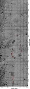 |
Fig. 1 Map of Ryugu between 50° north and 50° south. Red markings are fractures, mapped on available high-resolution images. This image is a compilation of a global Ryugu mosaic and the high-resolution images we worked on. For more information, see Sects. 1 and 2. The names of the individual images are listed in Appendix C. It is rotated for better visibility, so north is to the left and east is to the top. |
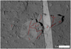 |
Fig. 2 Mapping example, with fracture segments in red. Composition of three Hayabusa2 images: hyb2_onc_20180921_025306_tvf_l2d, hyb2_onc_20181015_140115_tvf_l2d, and hyb2_onc_20181015_140218_tuf_l2d. The largesttwo boulders shown in this image are likely a fragmented boulder that was split in two along a fracture between the boulders (not mapped). The presence of two large boulders at such a close distance is most easily explained by them belonging to a single block (Ruesch et al. 2020; Rüsch & Bickel 2023). |
2.2 Mapping uncertainties
There are some difficulties associated with the fracture orientation results in Sect. 3.1: shadows cast by small ridges, overhangs, or layers could be mistaken for fractures. Shadows are most prominent when the Sun is low, and thus shines directly from the west or east, so this could introduce a bias into the observed north-south orientation. The north-south fractures may have a better visibility. Delbo et al. (2022) discuss this for Bennu and state that, since fractures are identified at different latitudes and they use images from two different phase angles, this potential bias cannot explain the observed orientations alone. They also minimized this problem by using images from two different times of day, resulting in two different phase angles. Hayabusa2 typically observed Ryugu’s surface from the direction of the Sun (rather than orbiting its target like OSIRIS-REx), resulting in low phase angle data and a narrow shadow width, which should minimize this problem.
It is also possible that due to limited image resolution some ridges, overhangs, or layers in the boulders could be mistaken for fractures. However, these features can also be part of the weathering morphology of the regolith, similar to fractures. In the other case that these features are pristine structures in the primordial bedrock with a potentially preferred orientation, they would not contain information about the weathering mechanism, but could shine a light on the geological evolution of Ryugu.
The mapping was conducted by the first author of this article, a trained geoscientist, and the results were discussed with the team, which consists of experienced planetary scientists and geologists. To verify the mapping, it was independently repeated on seven images by another coauthor. The second mapping found a similar number of fractures and mapped 70% of the fractures found in the first mapping. Importantly, a north–south orientation could be found in both of these mappings (see Figs. B.2 and B.1).
Another source of error could be a bias in the identification of the selection of fractures (de Lange et al. 2018) because the first author was aware of the findings from Delbo et al. (2022). Such a bias was somewhat quantified by taking ten images and redoing the mapping with randomly rotated images, so that the mapper does not know which way is north. In this setup, 81.3% of fractures were reidentified, suggesting that the influence of this potential bias is not too large.
Furthermore, mapping a 3D environment onto 2D images leads to oversimplification (Ruesch et al. 2020). In this study, fractures are identified as broken lines, but in reality, they are planes. It is assumed here that a mapped fracture with a north-south orientation corresponds to a fracture plane with an east-west pointing normal. This geometry has also been assumed by previous investigations on Bennu (Delbo et al. 2022) and follows models of thermal fracturing (El Mir et al. 2019; Uribe-Suárez et al. 2021; Ravaji et al. 2019). However, due to an arbitrarily complex geometry of scene, boulder, and fracture, it is possible that real fracture planes are different from our simple aforementioned geometrical assumption.
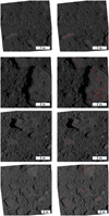 |
Fig. 3 Selection of mapped images. Mapped fractures are red. North is up. The image names are, from top to bottom: hyb2_onc_20190516_015610_tvf_l2d, hyb2_onc_20190711_002204_tvf_l2d, hyb2_onc_20190613_015921_tvf_l2d, and hyb2_onc_20190308_031420_tvf_l2d. |
2.3 Data processing
Once the mapping was completed, the fracture coordinates were exported from QGIS. This data was then read and processed with Python. The lengths, li, of the ith fracture segment were obtained via the euclidean norm on the map-projected images (see Eq. (1)). This assumes that Ryugu is spherical, which Ryugu is not. However, since the fractures are small (cm–m) and cluster around the equator, the resulting error is negligible. After this, the segment lengths were summed up to compute the total length of a fracture. The orientation, αi, of a fracture segment was calculated with Eq. (2) via the difference of the respective x1,2 and y1,2 coordinates of the fracture segment points, again assuming a spherical body with a radius of 450 m.
 (1)
(1)
 (2)
(2)
Once all the fracture orientations were calculated, they were plotted in rose diagrams. The length distribution plots were done by plotting the cumulative sum of the fractures against their length in a double logarithmic plot.
2.4 Fracture propagation model
The fracture propagation model of Delbo et al. (2022) was used to model fracture growth on Ryugu. The model uses the Paris law of fracture growth (Paris & Erdogan 1963) to estimate the timescale in which Ryugu’s current fracture population grew. For this, a stress intensity factor, KI, is calculated from a number of thermophysical parameters (see Table 1). Delbo et al. (2022) differentiate between horizontal and vertical fractures and find that the horizontal fractures grow orders of magnitude faster. Therefore, this work focuses only on horizontal fractures. Also, vertical fracture length is not observable in remote sensing data. The model usually simulates the growth of a fracture population, but to showcase its basic functionality a singular fracture is modeled in Fig. 4.
To apply this model to Ryugu, different thermophysical parameters had to be used, most notably the rotational period of 7.636 h (which differs from Bennu’s 4.296 h), resulting in a measured daily temperature variation of 97 K (Grott et al. 2019) compared to 70 K on Bennu. The total number of boulders was provided by data from Michikami et al. (2019; compared to DellaGiustina et al. 2020 for Bennu).
To correctly estimate other thermophysical properties of the boulders on Ryugu (and Bennu) is no easy task, since even the properties for different boulders on Ryugu can vary quite significantly (Sakatani et al. 2021; Ishizaki et al. 2023). Nevertheless, important parameters from the literature are compiled in Table 1 and comprise results from Hayabusa2’s MARA radiometer (Grott et al. 2019) and laboratory measurements on Ryugu samples that were brought to Earth by Hayabusa2 (Nakamura et al. 2023). In accordance with Delbo et al. (2014), the Paris law’s exponent and prefactor as well as the Poisson ratio, v, were taken from a CM chondrite. In the methods section of Delbo et al. (2022), the fracture-propagation model is described in more detail.
The final model parameters used in this study are listed in Table 2. The thermal inertia, Γ, rotation period, P, and diurnal temperature difference, ∆T, were taken from Grott et al. (2019). The heat capacity, Cp, thermal expansion coefficient, α, and Young’s modulus, E, were taken from lab work on Ryugu samples by Nakamura et al. (2023). The density, p, and Poisson ratio, v, are the same as in Delbo et al. (2022).
Ryugu’s parameters compiled for the fracture-propagation model.
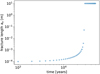 |
Fig. 4 Simulated growth of a singular fracture over 50 000 yr on Bennu, in a cylindrical boulder that has a diameter of 2 m and a length of 10 m. After about 30 000 yr, the maximum length of 10 m is reached and the fracture cannot grow further. |
3 Results and interpretation
3.1 Fracture orientation
The mapping resulted in a QGIS shape file, containing 1521 fractures, with a total of 4195 fracture segments. The orientations of these segments were computed and are plotted in Fig. 5. It shows a very strong and unambiguous north-south orientation. More than 66% of fractures here are oriented directly north-south (with a maximum deviation of 15° from a true north-south orientation). This is similar to the results Delbo et al. (2022) found for asteroid Bennu, Eppes et al. (2015) for Mars, and McFadden et al. (2005) for terrestrial deserts in North America. This is discussed more in Sect. 4.1.
The strong north-south preference in Fig. 5 is strong evidence for a thermal origin of these fractures. The eastern side of the observed boulders heats up in the morning, the western side in the evening, and the fractures form orthogonal to the main stress axis.
As was mentioned in Sect. 2.2, some of the mapped features might be mistaken overhangs, ridges, or layers. In the unlikely worst case that all of the mapped features are in reality ridges, overhangs, or layers, and not fractures, this would still lead to the conclusion that weathering on Ryugu somehow shows a preferred north-south orientation. Nonetheless, this would hint that the thermal influence via the sunlight in the morning or evening plays a role in the weathering of the small-body regolith. Or, in the case of pristine structures, this would mean that some mechanism in Ryugu’s formation has created these aligned, nonrandom structures.
3.2 Fracture length distribution
Following Delbo et al. (2022), the fractures were also evaluated regarding their length. Figure 6 is a reproduction of Fig. 3 from Delbo et al. (2022), with our Ryugu fracture data added. The graph shows the cumulative number of fractures and fracture segments plotted against their length. The data by Delbo et al. (2022) produced from Bennu (black and gray in Fig. 6) and the data we produced from Ryugu are similar, indicating that a partial mapping is enough to discover the underlying length distribution. Moreover, even though the mapping conducted in this work was not based on a global dataset of Ryugu, the length distribution that was found is still very similar to the global mapping by Delbo et al. (2022).
This suggests that, similar to findings for Bennu, the observed length distributions in Fig. 6 can be split into two parts depending on the fracture size (Fig. 7): the fracture lengths above approximately 3–4 m can be described by a power law and the fracture lengths below 3–4 m can be described with an exponential law. Since the largest fractures can only ever be as long as the diameter of the fractured boulder and since the boulder size frequency distribution is governed by a power law (Michikami et al. 2019), the fracture size above a certain size has to be a power law too. Below this threshold, the fracture lengths can be described by an exponential law, which was also found on comet 67P by Attree et al. (2018) and Matonti et al. (2019) and thought to be typical for a thermal origin (Delbo et al. 2022). At the lowest end of the fracture length distribution there is also a small part that is not described well by the exponential law, due to the resolution limit of the images, at which the fractures cannot be detected reliably.
Overall, the compared length distributions of fractures in boulders on Ryugu and Bennu in Fig. 7 are quite similar, implying that the underlying formation mechanisms are similar. This is not surprising, since Bennu and Ryugu are similar too in terms of their bulk composition (Kitazato et al. 2019, 2021; Hamilton et al. 2019) and heliocentric distances (Watanabe et al. 2019; Barnouin et al. 2019). The observed fractures on Ryugu are smaller than on Bennu, which could be explained by the higher resolution of the Hayabusa2 Ryugu images compared to the mosaic used to study Bennu. This is probably also the reason why a comparable amount of fractures was observed in both studies, even though the Ryugu dataset was not global. Michikami et al. (2019) complements this, by observing more boulders on Ryugu than DellaGiustina et al. (2020) did on Bennu, allowing for more fractures in boulders to exist on Ryugu. This is not surprising, since Ryugu’s surface is approximately three times larger than Bennu’s. The comparison of the two different fracture populations is difficult, since they are not normalized to the same area or boulder number; however, we can compare the underlying distributions, as is done in Table 3. This assumes that the fractures we mapped are representative of the entire surface of Ryugu.
The fracture length distribution of Ryugu is described with the power law  , with N0 = 988 and γ = −2.72, and the exponential law N = N1 exp(Lxβ), with N1 = 1788 and β = −1.475, compared to γ = −2.4 and β = −0.585 from Delbo et al. (2022). Michikami et al. (2019) find that γ = −2.65 for the boulder diameter distribution on Ryugu, which is in good agreement with our fracture length value of γ = −2.72. N is the cumulative number of fractures, and N0 and N1 are constants. The parameters are compiled in Table 3.
Parameters used for the fracture-propagation model.
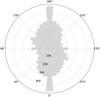 |
Fig. 5 Orientation of 4195 mapped fractures segments on Ryugu. North is up. The distribution is point-symmetrical since every fracture that points north also points south etc. |
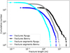 |
Fig. 6 Cumulative distribution of the length of fractures and fracture segments. The gray and black curves are from Delbo et al. (2022) and the blue curves are from this work on Ryugu. Overall, the fracture distributions are similar. The fractures found on Ryugu are generally smaller, which might be explained by higher-resolution images. |
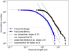 |
Fig. 7 Cumulative distribution of the length of fractures and fracture segments. The gray and black curves are from Delbo et al. (2022) and the blue curves are from this work on Ryugu. The dashed yellow and blue lines are power laws, fitted to the larger part of the plot. The dash-dotted red and green lines are exponential laws, fitted to the smaller part of the curves. |
3.3 Fracture propagation model
In Fig. 8, by Delbo et al. (2022), the modeled fracture growth after 10 000 yr on Bennu is shown. The plot shows the fracture length versus their accumulated number. The model starts with an initial microfracture distribution typical for chondrites ranging between 10−6 and 4 × 10⁻⁴ m (Bryson et al. 2018). The total amount of boulders, and therefore fractures, is based on data by DellaGiustina et al. (2020) and Michikami et al. (2019). The model then calculates the expected fracture growth and resulting fracture length distribution after a set duration. The modeled green curve in Fig. 8 has moved to slightly larger values compared to the initial blue microfracture distribution. The black and gray curves are the observed fracture length distributions of Bennu and Ryugu, respectively, whereas the yellow curve to the right is the observed boulder diameter distribution of Bennu, representing the maximum possible lengths of fractures.
When applying the model to Ryugu by using the compiled parameters of Ryugu in Table 2, the model output changes significantly. This results in a different fracture length distribution, plotted in Fig. 9, showing that Ryugu’s fractures grew to the observed sizes in the last 1000 yr. This seems unlikely, as Delbo et al. (2022) computed timescales that are almost two orders of magnitude higher for Bennu. This implies that some thermophysical parameters do not represent Ryugu’s average boulder properties well. This might be due to scale dependence: the values measured on a millimeter-large grain by Nakamura et al. (2023) might not represent a meter-sized boulder well (Otto et al. 2023).
Since the result of the model is strongly influenced (see Appendix A and Fig. 9) by the measured thermal expansion coefficient, α, and Young’s modulus, E, values (Table 2) of Ryugu, it seems prudent to pick the tried and tested values of 5 × 10⁻⁶ K−1 for the thermal expansion coefficient, α, and 10 GPa for Young’s modulus, E, of Bennu for Ryugu.
When picking these two values and otherwise identical parameters to Table 2 for Ryugu, the obtained length distribution in Fig. 10 is reasonable. The observed fracture lengths are somewhat larger compared to Bennu in Fig. 8, suggesting that the larger diurnal temperature variations on Ryugu accelerate fracture growth compared to those on Bennu. For this case, the model computes that a thermal fracture that needs 47 000 yr to grow to a length of 0.3 m on Bennu would grow to this length in about 30 000 yr on Ryugu. This, with the observed fracture distribution on Ryugu, seen in Fig. 6, suggests that the fracture growth timescale on Ryugu is faster than the 40 000-yr timescale of Bennu, as is modeled by Delbo et al. (2022). The fracture growth timescale here is the time needed for a 3 × 10⁻⁵ m long fracture to grow to a length of 0.3 m.
After considering these modeled scenarios (Figs. 8–11) the results in Fig. 10 seem realistic and reasonable. The slightly faster fracturing timescale of 30 000–40 000 yr can be explained by the increase in diurnal temperature change due to the longer period of Ryugu.
The physically implausible result in Fig. 9 is explained by inadequate values for the thermal expansion coefficient, α, and Young’s modulus, E. This is further discussed in Sect. 4.3 and Appendix A.
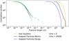 |
Fig. 8 Modeling of the evolution of a length distribution of fractures. Here, Bennu is modeled, exactly as in Delbo et al. (2022). The parameters used are listed in Table 2. The gray curve is the initial random distribution of microscopic fractures at time 0. The green curve is the modeled fracture distribution after 10 000 yr. The blue and black curves are the mapped fracture distributions of Ryugu and Bennu, respectively. The yellow curve represents the maximum possible value, that is, the diameter distribution of boulders on Bennu. Modeled values are dotted. |
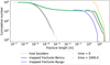 |
Fig. 9 Modeling of the evolution of a length distribution of fractures. Here, Ryugu is modeled, with the model parameters from Table 2. The modeled green curve reaches the observed fracture length values after about 1000 yr. This does not seem plausible, because all boulders should then be entirely fractured, which is not supported by observations. This mismatch can be explained by the choice of modeling parameters that appear to be unsuitable for this model (see Sect. 4.3 and Appendix A). The gray curve is the initial random distribution of microscopic fractures at time 0. The green curve is the modeled fracture distribution after 1000 yr. The blue and black curves are the mapped fracture distributions of Ryugu and Bennu, respectively. The yellow curve represents the maximum possible value, that is, the diameter distribution of boulders on Ryugu. Dotted values are modeled. The modeled values and the yellow host boulder distribution are now larger, since the boulder data from Michikami et al. (2019) is used, with more boulders found on Ryugu than on Bennu. |
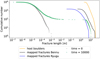 |
Fig. 10 Modeling of the evolution of a length distribution of fractures. Here, Ryugu is modeled, with Ryugu’s temperature difference and period from Table 2 and otherwise identical parameters to Bennu, as is discussed in Sect. 3.3. The gray curve is the initial random distribution of microscopic fractures at time 0. The green curve is the modeled fracture distribution after 10 000 yr. The blue and black curves are the mapped fracture distributions of Ryugu and Bennu, respectively. The yellow curve represents the maximum possible value, that is, the diameter distribution of boulders on Ryugu. Dotted values are modeled. The modeled values and the yellow host boulder distribution are now larger, since the data from Michikami et al. (2019) is now used, with more boulders found on Ryugu than on Bennu. |
4 Discussion
4.1 Fracture orientation
This work finds an unambiguous north-south orientation for Ryugu’s fractures, whereas Delbo et al. (2022) find a northwest-southeast direction for Bennu’s fractures. They discuss that this could be due to changes in Bennu’s orbit in the last hundred thousand years, which would imply that Ryugu’s orbit was more stable in the recent past. Okazaki et al. (2023) confirms this with an age of 5 million years for Ryugu’s current orbit. However, the north-south orientations found by McFadden et al. (2005), Eppes et al. (2015) and Ruesch et al. (2020) for Earth, Mars, and the Moonalso seem to be less pronounced, which suggests that there might be another phenomenon contributing to the strong orientation found on Ryugu in Fig. 5 or that the weathering phenomena under the atmosphere on Earth and Mars complicate the processes (see also Sect. 2.2 about uncertainties in the mapping process).
4.2 Fracture length distribution
Overall, the compared length distributions of fractures in boulders on Ryugu and Bennu in Fig. 7 are similar, implying that the underlying formation mechanisms may be similar. This is not surprising, since Bennu and Ryugu are rather similar in their composition, structure, heliocentric distance, and boulder population (Watanabe et al. 2019; Barnouin et al. 2019; Michikami et al. 2019; DellaGiustina et al. 2020). The observed fractures on Ryugu are smaller than on Bennu, which could be explained by the higher resolution (up to 1 cm per pixel, Kameda et al. 2016) of the Hayabusa2 Ryugu images compared to the mosaic used to study Bennu (5 cm per pixel, Delbo et al. 2022). This is probably also a reason why a comparable number of fractures was observed in both studies, even though the Ryugu dataset was not global. Michikami et al. (2019) complements this by observing more boulders on Ryugu than DellaGiustina et al. (2020) did on Bennu, allowing for more fractures in boulders to exist on Ryugu. This is not surprising, since Ryugu’s surface is about three times larger than Bennu’s.
The fracture length distribution on Bennu as well as Ryugu is best described with a exponential law for fractures below about 3–4 m, as is seen in Fig. 7. Exponential laws have been used before to describe thermally induced fractures on comets (Attree et al. 2018; Matonti et al. 2019). This exponential law then gets cut by a power law toward larger lengths, since fractures in boulders cannot grow limitlessly and can only ever be as large as their host boulder. Therefore, the fracture length distribution above a certain size can be described with the same power law that describes the boulder diameter (see Table 3).
4.3 Fracture propagation model
As is shown in Fig. 9, the values for Ryugu’s thermal expansion coefficient, α, and Young’s modulus, E, in Table 2 do not lead to reasonable results, because all boulders should then be entirely fractured after 1000 yr, which is not supported by observations (compare Fig. 2). The material values from the returned Ryugu samples provided by Nakamura et al. (2023) for Young’s modulus and the thermal expansion coefficient cause the model to accelerate the fracture growth to values larger than is physically reasonable. This is confirmed by our sensitivity analysis in Appendix A, where the thermal expansion coefficient has the largest sensitivity index by orders of magnitude, which means it has a comparatively large influence on the model output.
This might be because the measured values by Nakamura et al. (2023) were obtained from a millimeter-sized grain in a terrestrial laboratory, whereas the values used by Delbo et al. (2022) are estimated bulk values from meteorites, which may describe the modeled objects better as they produce reasonable results in Figs. 8 and 10. One possible reason for this could be that the data recorded by Nakamura et al. (2023) did not factor in the porosity and shape characteristics of the boulders. Another contributing factor might be the scale-dependent nature of the measurements: values obtained from tiny millimeter-sized grains might not accurately reflect the properties of much larger meter-sized boulders, as is suggested by Otto et al. (2023). Furthermore, recently Le Pivert-Jolivet et al. (2023) showed that the subsurface of Ryugu, which would include boulder interiors, can contain pristine fractures. This could mean that we overestimate the fracture growth timescales, since we assume initially microscopic fractures.
Delbo et al. (2022) estimated uncertainties for the parameters used. For the thermal expansion coefficient, which is the largest source of uncertainty (see Table A.1), they considered a lower value of 2 × 10⁻⁶ K−1 and an upper value of 8 × 10⁻⁶ K−1 from Opeil et al. (2020). These values result in a lower fracturing time estimate of 7000 yr and an upper estimate of 290 000 yr. Consequently, the uncertainty is estimated to be around −33 000 yr or +240 000 yr (from uncertainty in the thermal expansion coefficient). Although this uncertainty is substantial, assuming the worst case scenario with the reported age of 40 000 yr + 240 000 yr of uncertainty would still suggest that thermal fracturing is a fast process on geological timescales. Regarding the comparison between Ryugu and Bennu, if one assumes similar thermophysical properties, it would still imply that fractures grow slightly faster on Ryugu due to the increased period and resulting higher temperature difference. This would only change if there is a large systematic difference of thermo-physical properties of Ryugu and Bennu, which does not seem likely.
It should be noted that the value of 2.6 × 10⁻⁵ K−1 for Ryugu by Nakamura et al. (2023) is even larger than the upper measured value for chondrites by Opeil et al. (2020) and also outside of the ranges for typical rocks on earth (Robertson 1988). For this reason, this value is rejected and not used at all in the modeling.
Because these material values come with large uncertainties and to make a comparison of fracture formation on Bennu and Ryugu feasible, it is prudent to use identical values for Bennu’s and Ryugu’s thermal expansion coefficient and Young’s modulus. This leads to only well-constrained values being changed (Fig. 10) and allows us to estimate the timescale in which thermal fracturing takes place on Bennu and Ryugu. In this case, slightly shorter timescales (approx. 30 000 yr), as are reported by Delbo et al. (2022; approx. 40 000 yr), are calculated for Ryugu.
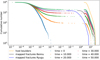 |
Fig. 11 Modeling of the evolution of a length distribution of fractures on Ryugu. The thermal expansion coefficient and Young modulus values are from Delbo et al. (2022) in Table 2. In this figure, every 10 000-yr step from 0 to 50 000 yr is shown. Dotted curves are the modeled values after 0 to 50 000 yr. Straight blue and black curves are the mapped fracture distributions of Ryugu and Bennu, respectively. The straight yellow curve represents the maximum possible value, that is, the diameter distribution of host boulders on Ryugu. |
5 Conclusions
This comparative study not only reinforces the significance of thermal rock fracturing but also highlights the dynamic and rapid processes at play within the near-Earth asteroid population. By corroborating these findings across two distinct asteroids, we contribute to a deeper understanding of the forces that govern the evolution of these enigmatic celestial bodies.
A fracture mapping effort similar to Delbo et al. (2022) on Bennu was applied to a second asteroid, Ryugu. 1521 fractures were mapped on Ryugu compared to 1475 on Bennu. Their fracture propagation model was employed to estimate timescales for fracture growth on Ryugu. This resulted in the following conclusions:
Ryugu’s surface is covered with fractured boulders. These fractures are not randomly distributed, but instead show a strong north-south orientation. The north-south orientation can be explained by a thermal fracture origin: the Sun heats up the boulders preferentially on the eastern side in the morning and on the western side in the evening. This leads to fracture growth perpendicular to the main thermal stress axis;
The fracture lengths distributions of boulders on Ryugu and Bennu are similar and can be described by comparable exponential and power laws. Even though our mapping on Ryugu was only local (in contrast to the global investigation by Delbo et al. 2022), a meaningful fracture length distribution could still be determined. However, there are some flaws in this process. Firstly, the mapped area size differed from the global investigation, potentially influencing the representativeness of our findings. Additionally, there were inherent challenges in fracture identification and the mapping process itself. The reliance on visual expertise, the interpretation of 2D images of a 3D environment, and the influence of visual expectations introduce ambiguities that may impact the accuracy of our results. Despite these limitations, the observed similarity between the fracture length distributions on Ryugu and Bennu suggests corresponding origins;
The timescale of the observed fracture growth can be approximated with the fracture propagation model by Delbo et al. (2022). The fracture propagation model estimates an even shorter timescale for fracture growth on Ryugu, about 30000–40000 yr, compared to the 40000–50000 yr on Bennu. The uncertainty on these values is large (up to 250 000 yr) due to large uncertainty about the exact values of the thermophysical parameters. Even with this uncertainty, the model still suggests that thermal fracturing is a geologically fast process. The comparison between Ryugu and Bennu does not suffer much from this uncertainty, since the uncertainty derives from the uncertainty of the exact values for the thermophysical parameters. Whatever the true values are in reality, due to the overall similarity of these two bodies, it’s likely that the thermophysical parameter values are similar too, which means that thermal fracturing is probably slightly faster on Ryugu than on Bennu. This is mainly induced by the larger diurnal temperature variation on Ryugu. The finding of evidence for thermal fracturing on Ryugu suggests that thermal fracturing is a common process on airless bodies that plays a significant role in shaping these two carbonaceous bodies’ surfaces on very short timescales.
Acknowledgements
We acknowledge the efforts by the Hayabusa2 team in developing and operating the mission and collecting and providing the data which made this work possible. We also gratefully acknowledge the constructive comments by O. Rüsch that helped improving the article. The first author was funded by DLR Berlin and the Asteroid Engineering Laboratory by Lulea University of Technology.
Appendix A Sensitivity analysis
To analyse how the parameters used in the fracture propagation model influence the resulting fracture growth and to understand why the fractures on Ryugu grow unrealistically fast in Fig. 9, we conducted a sensitivity analysis. For this, the first-order sensitivity index, Si, after Saltelli et al. (2007), was calculated (where i indexes the parameters analysed). Each of the parameters listed in Tab.2 was varied individually, while the other parameters remained constant, and the amount of time needed to grow a 10 m long fracture was measured. By dividing the change in the model output, ∆y, by the change in the parameter, ∆x, the influence of the parameter can be quantified:
 (A.1)
(A.1)
where ∆y is the model output parameter, in this case the fracturing time needed to split a 10 m long boulder, and ∆x is the specific parameter that was varied in ten equal steps, listed in Tab. A.1. We note that if a parameter, y, does not vary with a changing x, the sensitivity index is 0.
Seven of the analysed parameters are positively correlated with the fracture growth speed, meaning a higher value leads to a shorter fracturing time of the 10 m long boulder. They include the Paris law prefactor, C, density, ρ, heat capacity, Cp, thermal expansion coefficient, α, Poisson ratio, v, Young’s modulus, E, and the temperature difference, ∆T.
Three of the parameters are negatively correlated with the fracture growth speed, meaning that higher values lead to longer fracturing times. Those are the Paris law exponent, n, thermal inertia, Γ, and rotation period, P. Notably, P is the only dependency that grows approximately linearly. Also, in reality an increase in the period, P, would lead to an increase in the temperature difference, ∆T, which is not considered in this sensitivity analysis. Therefore, the sensitivity index obtained for P has to be considered with caution.
The obtained indices help to explain the results of the model in section 3.3. The parameter with the largest influence on the output is the thermal expansion coefficient, α. This is also the parameter in tables 1 and 2 with a large discrepancy between Delbo et al. (2022) and the values measured by Nakamura et al. (2023). This explains the questionable fracture growth times illustrated in Fig. 9.
C, n, and v also have large sensitivity index values in Tab.A.1, but were not changed in the modeling of Ryugu and Bennu, and therefore have no effect on the results there. The rotation period, P, also has a relatively large value for the sensitivity index, and influences the temperature difference, ∆T. However, for clarity, these values were considered independently. Young’s modulus, E, also has a sizeable sensitivity index and the values in Tab.2 also differ by almost 50%. But since the used value is smaller than the one used by Delbo et al. (2022), it contributes to mitigating the large effect caused by the change in α. The influences of the thermal inertia, Γ, density, ρ, and heat capacity, Cp, are quite small.
Sensitivity indices for the analysed parameters after Saltelli et al. (2007).
The unit of these sensitivity indices is year/unit, in which unit is the unit of the specific parameter. A large value means that a change in this parameter has a large influence on the resulting fracture growth. For reference, the rightmost column lists the actual value with the specific unit of the parameter used in the model.
Appendix B Mapping verification
The mapping detailed in section 2.1 was initially conducted entirely by the first author to ensure consistency. For validation, a separate coauthor independently performed visual fracture identification and mapping. This second mapping process took place on seven images of Ryugu, strategically chosen to encompass regions with diverse geological characteristics, with variations in boulder density. Utilizing the QGIS software package, this independent effort followed the same mapping procedure outlined in section 2.1.
This resulted in two key observations: (i) on average the second coauthor identified almost the same number of fractures (21.43) compared to the initial mapping by the first coauthor (22.3); and (ii) across the seven selected areas, the second coauthor successfully identified 70% of the fractures that were also mapped by the first coauthor, whereas the first author only identified 58% of the fractures mapped by the coauthor, still indicating a substantial level of agreement between the two mapping efforts. An example of this is showcased in figure B.1, where blue arrows indicate fractures that were not found by the second mapping.
The orientation of fractures in this mapping verification was also studied. In figure B.2a, where the orientation of fractures in the original mapping is plotted, the north-south orientation is heavily pronounced. While the north-south trend can still be observed in figure B.2b, it’s a lot less pronounced.
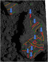 |
Fig. B.1 Example of the mapping verification. Fractures mapped by the first author are red; those by the second author are green. Blue arrows mark fractures not found by the second mapping. The image width is about 5 meters. |
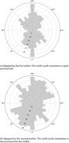 |
Fig. B.2 Comparison of fracture orientation for a selection of seven images mapped by two different authors. |
Appendix C List of images
Listing 1: High-resolution Hayabusa2 ONC images were used in this work. The data can be retrieved from JAXA at: https://data.darts.isas.jaxa.jp/pub/hayabusa2/ onc_bundle/
’hyb2_onc_20180806_225848_tvf_12d’,
’hyb2_onc_20180921_025306_tvf_12d’,
’hyb2_onc_20180921_025442_tuf_12d’,
’hyb2_onc_20180921_033442_tvf_12d’,
’hyb2_onc_20180921_033618_tuf_12d’,
’hyb2_onc_20180921_034938_tvf_12d’,
’hyb2_onc_20180921_035114_tuf_12d’,
’hyb2_onc_20180921_040154_tvf_12d’,
’hyb2_onc_20180921_040402_tvf_12d’,
’hyb2_onc_20180921_040634_tvf_12d’,
’hyb2_onc_20180921_041826_tvf_12d’,
’hyb2_onc_20180921_042106_tvf_12d’,
’hyb2_onc_20180921_042418_tvf_12d’,
’hyb2_onc_20180921_042730_tvf_12d’,
’hyb2_onc_20180921_043010_tvf_12d’,
’hyb2_onc_20181003_003036_tvf_12d’,
’hyb2_onc_20181003_003212_tuf_12d’,
’hyb2_onc_20181003_012044_tvf_12d’,
’hyb2_onc_20181003_012220_tuf_12d’,
’hyb2_onc_20181003_013540_tvf_12d’,
’hyb2_onc_20181003_013553_twf_12d’,
’hyb2_onc_20181003_013716_tuf_12d’,
’hyb2_onc_20181003_014756_tvf_12d’,
’hyb2_onc_20181003_015004_tvf_12d’,
’hyb2_onc_20181003_015212_tvf_12d’,
’hyb2_onc_20181003_015420_tvf_12d’,
’hyb2_onc_20181003_015653_tvf_12d’,
’hyb2_onc_20181003_021156_tvf_12d’,
’hyb2_onc_20181003_021436_tvf_12d’,
’hyb2_onc_20181003_021748_tvf_12d’,
’hyb2_onc_20181003_022100_tvf_12d’,
’hyb2_onc_20181003_022340_tvf_12d’,
’hyb2_onc_20181003_022652_tvf_12d’,
’hyb2_onc_20181015_130717_twf_12d’,
’hyb2_onc_20181015_132213_twf_12d’,
’hyb2_onc_20181015_132337_tuf_12d’,
’hyb2_onc_20181015_133045_twf_12d’,
’hyb2_onc_20181015_133209_tuf_12d’,
’hyb2_onc_20181015_133625_tvf_12d’,
’hyb2_onc_20181015_133833_tvf_12d’,
’hyb2_onc_20181015_134041_tvf_12d’,
’hyb2_onc_20181015_134616_tvf_12d’,
’hyb2_onc_20181015_134627_twf_12d’,
’hyb2_onc_20181015_134638_txf_12d’,
’hyb2_onc_20181015_134655_tpf_12d’,
’hyb2_onc_20181015_134707_tbf_12d’,
’hyb2_onc_20181015_134718_tuf_12d’,
’hyb2_onc_20181015_134935_tvf_12d’,
’hyb2_onc_20181015_135038_tuf_12d’,
’hyb2_onc_20181015_135255_tvf_12d’,
’hyb2_onc_20181015_135358_tuf_12d’,
’hyb2_onc_20181015_140115_tvf_12d’,
’hyb2_onc_20181015_140218_tuf_12d’,
’hyb2_onc_20181025_015814_tuf_12d’,
’hyb2_onc_20181025_021134_tvf_12d’,
’hyb2_onc_20181025_021310_tuf_12d’,
’hyb2_onc_20181025_022006_tvf_12d’,
’hyb2_onc_20181025_022142_tuf_12d’,
’hyb2_onc_20181025_022558_tvf_12d’,
’hyb2_onc_20181025_022806_tvf_12d’,
’hyb2_onc_20181025_023014_tvf_12d’,
’hyb2_onc_20181025_030628_tuf_12d’,
’hyb2_onc_20190221_205818_tvf_12d’,
’hyb2_onc_20190221_205954_tuf_12d’,
’hyb2_onc_20190221_213610_tvf_12d’,
’hyb2_onc_20190221_213746_tuf_12d’,
’hyb2_onc_20190221_215106_tvf_12d’,
’hyb2_onc_20190221_215242_tuf_12d’,
’hyb2_onc_20190221_215938_tvf_12d’,
’hyb2_onc_20190221_220022_tnf_12d’,
’hyb2_onc_20190221_220114_tuf_12d’,
’hyb2_onc_20190221_220322_tvf_12d’,
’hyb2_onc_20190221_220530_tvf_12d’,
’hyb2_onc_20190308_021228_tvf_12d’,
’hyb2_onc_20190308_021404_tuf_12d’,
’hyb2_onc_20190308_025052_tvf_12d’,
’hyb2_onc_20190308_025228_tuf_12d’,
’hyb2_onc_20190308_030548_tvf_12d’,
’hyb2_onc_20190308_030724_tuf_12d’,
’hyb2_onc_20190308_031420_tvf_12d’,
’hyb2_onc_20190308_031504_tnf_12d’,
’hyb2_onc_20190308_031556_tuf_12d’,
’hyb2_onc_20190308_031804_tvf_12d’,
’hyb2_onc_20190308_032012_tvf_12d’,
’hyb2_onc_20190308_032220_tvf_12d’,
’hyb2_onc_20190308_032448_tvf_12d’,
’hyb2_onc_20190308_032604_tvf_12d’,
’hyb2_onc_20190308_032829_tvf_12d’,
’hyb2_onc_20190308_033010_tvf_12d’,
’hyb2_onc_20190308_033650_tvf_12d’,
’hyb2_onc_20190308_033701_twf_12d’,
’hyb2_onc_20190516_011850_tvf_12d’,
’hyb2_onc_20190516_012026_tuf_12d’,
’hyb2_onc_20190516_015610_tvf_12d’,
’hyb2_onc_20190516_015746_tuf_12d’,
’hyb2_onc_20190516_021106_tvf_12d’,
’hyb2_onc_20190516_021222_tbf_12d’,
’hyb2_onc_20190516_021938_tvf_12d’,
’hyb2_onc_20190516_022010_txf_12d’,
’hyb2_onc_20190516_022114_tuf_12d’,
’hyb2_onc_20190516_022322_tvf_12d’,
’hyb2_onc_20190530_004754_tvf_12d’,
’hyb2_onc_20190530_012722_tvf_12d’,
’hyb2_onc_20190530_012858_tuf_12d’,
’hyb2_onc_20190530_014218_tvf_12d’,
’hyb2_onc_20190530_014335_tbf_12d’,
’hyb2_onc_20190530_015434_tvf_12d’,
’hyb2_onc_20190530_015642_tvf_12d’,
’hyb2_onc_20190530_015850_tvf_12d’,
’hyb2_onc_20190530_020058_tvf_12d’,
’hyb2_onc_20190530_022626_tvf_12d’,
’hyb2_onc_20190530_023543_tvf_12d’,
’hyb2_onc_20190530_023555_twf_12d’,
’hyb2_onc_20190530_023606_txf_12d’,
’hyb2_onc_20190530_023623_tpf_12d’,
’hyb2_onc_20190530_023635_tbf_12d’,
’hyb2_onc_20190530_023646_tuf_12d’,
’hyb2_onc_20190530_023724_tvf_12d’,
’hyb2_onc_20190530_023735_twf_12d’,
’hyb2_onc_20190530_023746_txf_12d’,
’hyb2_onc_20190530_023804_tpf_12d’,
’hyb2_onc_20190530_023815_tbf_12d’,
’hyb2_onc_20190530_023826_tuf_12d’,
’hyb2_onc_20190530_023904_tvf_12d’,
’hyb2_onc_20190530_023915_twf_12d’,
’hyb2_onc_20190530_023927_txf_12d’,
’hyb2_onc_20190530_023944_tpf_12d’,
’hyb2_onc_20190530_023956_tbf_12d’,
’hyb2_onc_20190530_024007_tuf_12d’,
’hyb2_onc_20190530_024405_tvf_12d’,
’hyb2_onc_20190530_024416_twf_12d’,
’hyb2_onc_20190530_024427_txf_12d’,
’hyb2_onc_20190530_024445_tpf_12d’,
’hyb2_onc_20190530_024456_tbf_12d’,
’hyb2_onc_20190530_024507_tuf_12d’,
’hyb2_onc_20190530_024618_tvf_12d’,
’hyb2_onc_20190530_024631_twf_12d’,
’hyb2_onc_20190530_024650_txf_12d’,
’hyb2_onc_20190530_024703_tnf_12d’,
’hyb2_onc_20190530_024722_tpf_12d’,
’hyb2_onc_20190530_024735_tbf_12d’,
’hyb2_onc_20190530_024754_tuf_12d’,
’hyb2_onc_20190613_002323_tuf_12d’,
’hyb2_onc_20190613_010043_tvf_12d’,
’hyb2_onc_20190613_010219_tuf_12d’,
’hyb2_onc_20190613_011539_tvf_12d’,
’hyb2_onc_20190613_011715_tuf_12d’,
’hyb2_onc_20190613_012411_tvf_12d’,
’hyb2_onc_20190613_012423_twf_12d’,
’hyb2_onc_20190613_012547_tuf_12d’,
’hyb2_onc_20190613_012755_tvf_12d’,
’hyb2_onc_20190613_013003_tvf_12d’,
’hyb2_onc_20190613_013211_tvf_12d’,
’hyb2_onc_20190613_013419_tvf_12d’,
’hyb2_onc_20190613_015845_tvf_12d’,
’hyb2_onc_20190613_015928_tvf_12d’,
’hyb2_onc_20190613_020045_tvf_12d’,
’hyb2_onc_20190613_020156_tvf_12d’,
’hyb2_onc_20190613_020203_tvf_12d’,
’hyb2_onc_20190613_020210_tvf_12d’,
’hyb2_onc_20190613_020217_tvf_12d’,
’hyb2_onc_20190613_020224_tvf_12d’,
’hyb2_onc_20190613_020235_twf_12d’,
’hyb2_onc_20190613_020247_txf_12d’,
’hyb2_onc_20190613_020304_tpf_12d’,
’hyb2_onc_20190613_020315_tbf_12d’,
’hyb2_onc_20190613_020327_tuf_12d’,
’hyb2_onc_20190613_020404_tvf_12d’,
’hyb2_onc_20190613_020415_twf_12d’,
’hyb2_onc_20190613_020427_txf_12d’,
’hyb2_onc_20190613_020445_tpf_12d’,
’hyb2_onc_20190613_020456_tbf_12d’,
’hyb2_onc_20190613_020507_tuf_12d’,
’hyb2_onc_20190613_020545_tvf_12d’,
’hyb2_onc_20190613_020556_twf_12d’,
’hyb2_onc_20190613_020608_txf_12d’,
’hyb2_onc_20190613_020625_tpf_12d’,
’hyb2_onc_20190613_020636_tbf_12d’,
’hyb2_onc_20190613_020648_tuf_12d’,
’hyb2_onc_20190613_020815_tvf_12d’,
’hyb2_onc_20190613_020826_twf_12d’,
’hyb2_onc_20190613_020838_txf_12d’,
’hyb2_onc_20190613_020856_tpf_12d’,
’hyb2_onc_20190613_020907_tbf_12d’,
’hyb2_onc_20190613_020918_tuf_12d’,
’hyb2_onc_20190613_021659_tvf_12d’,
’hyb2_onc_20190613_021835_tuf_12d’,
’hyb2_onc_20190710_232532_tvf_12d’,
’hyb2_onc_20190711_000721_twf_12d’,
’hyb2_onc_20190711_000844_tuf_12d’,
’hyb2_onc_20190711_002204_tvf_12d’,
’hyb2_onc_20190711_002321_tbf_12d’,
’hyb2_onc_20190711_003036_tvf_12d’,
’hyb2_onc_20190711_003153_tbf_12d’,
’hyb2_onc_20190711_003212_tuf_12d’,
’hyb2_onc_20190711_003420_tvf_12d’,
’hyb2_onc_20190711_003628_tvf_12d’,
’hyb2_onc_20190711_003836_tvf_12d’,
References
- Attree, N., Groussin, O., Jorda, L., et al. 2018, A&A, 610, A76 [NASA ADS] [CrossRef] [EDP Sciences] [Google Scholar]
- Ballouz, R.-L., Walsh, K. J., Barnouin, O. S., et al. 2020, Nature, 587, 205 [Google Scholar]
- Barnouin, O. S.,, Daly, M. G., Palmer, E. E., et al. 2019, Nat. Geosci., 12, 247 [NASA ADS] [CrossRef] [Google Scholar]
- Basilevsky, A., Head, J., Horz, F., & Ramsley, K. 2015, Planet. Space Sci., 117, 312 [CrossRef] [Google Scholar]
- Bennett, C., DellaGiustina, D., Becker, K., et al. 2021, Icarus, 357, 113690 [NASA ADS] [CrossRef] [Google Scholar]
- Bruno, D. E., & Ruban, D. A. 2017, Planet. Space Sci., 135, 37 [NASA ADS] [CrossRef] [Google Scholar]
- Bryson, K. L., Ostrowski, D. R., & Blasizzo, A. 2018, Planet. Space Sci., 164, 85 [NASA ADS] [CrossRef] [Google Scholar]
- Cambioni, S., Delbo, M., Poggiali, G., et al. 2021, Nature, 598, 49 [NASA ADS] [CrossRef] [Google Scholar]
- de Lange, F. P., Heilbron, M., & Kok, P. 2018, Trends Cogn. Sci., 22, 764 [CrossRef] [Google Scholar]
- Delbo, M., Libourel, G., Wilkerson, J., et al. 2014, Nature, 508, 233 [Google Scholar]
- Delbo, M., Walsh, K. J., Matonti, C., et al. 2022, Nat. Geosci., 15, 453 [NASA ADS] [CrossRef] [Google Scholar]
- DellaGiustina, D. N., Emery, J. P., Golish, D. R., et al. 2019, Nat. Astron., 3, 341 [Google Scholar]
- DellaGiustina, D. N., Burke, K. N., Walsh, K. J., et al. 2020, Science, 370, eabc3660 [Google Scholar]
- El Mir, C., Ramesh, K., & Delbo, M. 2019, Icarus, 333, 356 [NASA ADS] [CrossRef] [Google Scholar]
- Eppes, M.-C., Willis, A., Molaro, J., Abernathy, S., & Zhou, B. 2015, Nature Comm., 6, 6712 [NASA ADS] [CrossRef] [Google Scholar]
- Grott, M., Knollenberg, J., Hamm, M., et al. 2019, Nat. Astron., 3, 971 [Google Scholar]
- Hamilton, V. E., Simon, A. A., Christensen, P. R., et al. 2019, Nat. Astron., 3, 332 [Google Scholar]
- Ho, T.-M., Jaumann, R., Bibring, J.-P., et al. 2021, Planet. Space Sci., 200, 105200 [NASA ADS] [CrossRef] [Google Scholar]
- Hörz, F., Basilevsky, A. T., Head, J. W., & Cintala, M. J. 2020, Planet. Space Sci., 194, 105105 [CrossRef] [Google Scholar]
- Ishizaki, T., Nagano, H., Tanaka, S., et al. 2023, Int. J. Thermophys., 44, 51 [NASA ADS] [CrossRef] [Google Scholar]
- Jawin, E. R., Walsh, K. J., Barnouin, O. S., et al. 2020, J. Geophys. Res.: Planets, 125, e06475 [CrossRef] [Google Scholar]
- Kameda, S., Suzuki, H., Takamatsu, T., et al. 2016, Space Sci. Rev., 208, 17 [Google Scholar]
- Kitazato, K., Milliken, R. E., Iwata, T., et al. 2019, Science, 364, 272 [Google Scholar]
- Kitazato, K., Milliken, R. E., Iwata, T., et al. 2021, Nat. Astron., 5, 246 [NASA ADS] [CrossRef] [Google Scholar]
- Kouyama, T., Tatsumi, E., Yokota, Y., et al. 2021, Icarus, 360, 114353 [NASA ADS] [CrossRef] [Google Scholar]
- Le Pivert-Jolivet, T., Brunetto, R., Pilorget, C., et al. 2023, Nat. Astron., 7, 1445 [Google Scholar]
- Libourel, G., Ganino, C., Delbo, M., et al. 2020, MNRAS, 500, 1905 [CrossRef] [Google Scholar]
- Matonti, C., Attree, N., Groussin, O., et al. 2019, Nat. Geosci., 12, 157 [NASA ADS] [CrossRef] [Google Scholar]
- McFadden, L., Eppes, M., Gillespie, A., & Hallet, B. 2005, GSA Bull., 117, 161 [NASA ADS] [CrossRef] [Google Scholar]
- Michikami, T., Honda, C., Miyamoto, H., et al. 2019, Icarus, 331, 179 [NASA ADS] [CrossRef] [Google Scholar]
- Molaro, J. L., Byrne, S., & Langer, S. A. 2015, J. Geophys. Res.: Planets, 120, 255 [NASA ADS] [CrossRef] [Google Scholar]
- Molaro, J., Byrne, S., & Le, J.-L. 2017, Icarus, 294, 247 [CrossRef] [Google Scholar]
- Molaro, J. L., Walsh, K. J., Jawin, E. R., et al. 2020, Nat. Commun., 11, 2913 [NASA ADS] [CrossRef] [Google Scholar]
- Nakamura, T., Matsumoto, M., Amano, K., et al. 2023, Science, 379, eabn8671 [CrossRef] [Google Scholar]
- Okada, T., Fukuhara, T., Tanaka, S., et al. 2016, Space Sci. Rev., 208, 255 [Google Scholar]
- Okazaki, R., Marty, B., Busemann, H., et al. 2023, Science, 379, eabo0431 [CrossRef] [Google Scholar]
- Opeil, C. P., Britt, D. T., Macke, R. J., & Consolmagno, G. J. 2020, Meteor. Planet. Sci., 55 [CrossRef] [Google Scholar]
- Otto, K. A., Matz, K.-D., Schroder, S. E., et al. 2020, MNRAS, 500, 3178 [NASA ADS] [CrossRef] [Google Scholar]
- Otto, K., Ho, T.-M., Ulamec, S., et al. 2023, Earth Planets Space, 75, 51 [NASA ADS] [CrossRef] [Google Scholar]
- Paris, P., & Erdogan, F. 1963, J. Basic Eng., 85, 528 [CrossRef] [Google Scholar]
- QGIS Development Team 2023, QGIS Geographic Information System, (Open Source Geospatial Foundation), http://qgis.org [Google Scholar]
- Ravaji, B., Alí-Lagoa, V., Delbo, M., & Wilkerson, J. W. 2019, J. Geophys. Res.: Planets, 124, 3304 [NASA ADS] [CrossRef] [Google Scholar]
- Robertson, E. C. 1988, Thermal Properties of Rocks (United States Department of the interior Geological Survey) [Google Scholar]
- Rozitis, B., Ryan, A. J., Emery, J. P., et al. 2020, Sci. Adv., 6, eabc3699 [CrossRef] [Google Scholar]
- Ruesch, O., Sefton-Nash, E., Vago, J., et al. 2020, Icarus, 336, 113431 [NASA ADS] [CrossRef] [Google Scholar]
- Rüsch, O., & Bickel, V. T. 2023, Planet. Sci. J., 4, 126 [CrossRef] [Google Scholar]
- Saiki, T., Sawada, H., Okamoto, C., et al. 2013, Acta Astron., 84, 227 [NASA ADS] [CrossRef] [Google Scholar]
- Sakatani, N., Tanaka, S., Okada, T., et al. 2021, Nat. Astron., 5, 766 [NASA ADS] [CrossRef] [Google Scholar]
- Saltelli, A., Ratto, M., Andres, T., et al. 2007, Global Sensitivity Analysis. The Primer (Wiley) [CrossRef] [Google Scholar]
- Sasaki, S., Kanda, S., Hikuchi, H., et al. 2020, in Proceedings of the 51st Lunar and Planetary Science Conference [Google Scholar]
- Sasaki, S., Kanda, S., Hikuchi, H., et al. 2022, in Proceedings of the 34th International Symposium on Space Technology and Science [Google Scholar]
- Sugita, S., Honda, R., Morota, T., et al. 2019a, HAYABUSA2 Optical Navigation Camera (ONC) documentation, https://data.darts.isas.jaxa.jp/pub/hayabusa2/onc_bundle/browse/ [Google Scholar]
- Sugita, S., Honda, R., Morota, T., et al. 2019b, Science, 364, eaaw0422 [Google Scholar]
- Suzuki, H., Yamada, M., Kouyama, T., et al. 2018, Icarus, 300, 341 [NASA ADS] [CrossRef] [Google Scholar]
- Tatsumi, E., Kouyama, T., Suzuki, H., et al. 2019, Icarus, 325, 153 [NASA ADS] [CrossRef] [Google Scholar]
- Uribe-Suárez, D., Delbo, M., Bouchard, P.-O., & Pino-Muñoz, D. 2021, Icarus, 360, 114347 [CrossRef] [Google Scholar]
- Wada, K., Grott, M., Michel, P., et al. 2018, Progr. Earth Planet. Sci., 5, 1 [NASA ADS] [CrossRef] [Google Scholar]
- Watanabe, S.-i., Tsuda, Y., Yoshikawa, M., et al. 2017, Space Sci. Rev., 208, 3 [Google Scholar]
- Watanabe, S., Hirabayashi, M., Hirata, N., et al. 2019, Science, 364, 268 [NASA ADS] [Google Scholar]
- Yada, T., Abe, M., Okada, T., et al. 2021, Nat. Astron., 6, 214 [Google Scholar]
- Yokoyama, T., Nagashima, K., Nakai, I., et al. 2023, Science, 379, eabn7850 [CrossRef] [Google Scholar]
All Tables
All Figures
|
Fig. 1 Map of Ryugu between 50° north and 50° south. Red markings are fractures, mapped on available high-resolution images. This image is a compilation of a global Ryugu mosaic and the high-resolution images we worked on. For more information, see Sects. 1 and 2. The names of the individual images are listed in Appendix C. It is rotated for better visibility, so north is to the left and east is to the top. |
| In the text | |
|
Fig. 2 Mapping example, with fracture segments in red. Composition of three Hayabusa2 images: hyb2_onc_20180921_025306_tvf_l2d, hyb2_onc_20181015_140115_tvf_l2d, and hyb2_onc_20181015_140218_tuf_l2d. The largesttwo boulders shown in this image are likely a fragmented boulder that was split in two along a fracture between the boulders (not mapped). The presence of two large boulders at such a close distance is most easily explained by them belonging to a single block (Ruesch et al. 2020; Rüsch & Bickel 2023). |
| In the text | |
|
Fig. 3 Selection of mapped images. Mapped fractures are red. North is up. The image names are, from top to bottom: hyb2_onc_20190516_015610_tvf_l2d, hyb2_onc_20190711_002204_tvf_l2d, hyb2_onc_20190613_015921_tvf_l2d, and hyb2_onc_20190308_031420_tvf_l2d. |
| In the text | |
|
Fig. 4 Simulated growth of a singular fracture over 50 000 yr on Bennu, in a cylindrical boulder that has a diameter of 2 m and a length of 10 m. After about 30 000 yr, the maximum length of 10 m is reached and the fracture cannot grow further. |
| In the text | |
|
Fig. 5 Orientation of 4195 mapped fractures segments on Ryugu. North is up. The distribution is point-symmetrical since every fracture that points north also points south etc. |
| In the text | |
|
Fig. 6 Cumulative distribution of the length of fractures and fracture segments. The gray and black curves are from Delbo et al. (2022) and the blue curves are from this work on Ryugu. Overall, the fracture distributions are similar. The fractures found on Ryugu are generally smaller, which might be explained by higher-resolution images. |
| In the text | |
|
Fig. 7 Cumulative distribution of the length of fractures and fracture segments. The gray and black curves are from Delbo et al. (2022) and the blue curves are from this work on Ryugu. The dashed yellow and blue lines are power laws, fitted to the larger part of the plot. The dash-dotted red and green lines are exponential laws, fitted to the smaller part of the curves. |
| In the text | |
|
Fig. 8 Modeling of the evolution of a length distribution of fractures. Here, Bennu is modeled, exactly as in Delbo et al. (2022). The parameters used are listed in Table 2. The gray curve is the initial random distribution of microscopic fractures at time 0. The green curve is the modeled fracture distribution after 10 000 yr. The blue and black curves are the mapped fracture distributions of Ryugu and Bennu, respectively. The yellow curve represents the maximum possible value, that is, the diameter distribution of boulders on Bennu. Modeled values are dotted. |
| In the text | |
|
Fig. 9 Modeling of the evolution of a length distribution of fractures. Here, Ryugu is modeled, with the model parameters from Table 2. The modeled green curve reaches the observed fracture length values after about 1000 yr. This does not seem plausible, because all boulders should then be entirely fractured, which is not supported by observations. This mismatch can be explained by the choice of modeling parameters that appear to be unsuitable for this model (see Sect. 4.3 and Appendix A). The gray curve is the initial random distribution of microscopic fractures at time 0. The green curve is the modeled fracture distribution after 1000 yr. The blue and black curves are the mapped fracture distributions of Ryugu and Bennu, respectively. The yellow curve represents the maximum possible value, that is, the diameter distribution of boulders on Ryugu. Dotted values are modeled. The modeled values and the yellow host boulder distribution are now larger, since the boulder data from Michikami et al. (2019) is used, with more boulders found on Ryugu than on Bennu. |
| In the text | |
|
Fig. 10 Modeling of the evolution of a length distribution of fractures. Here, Ryugu is modeled, with Ryugu’s temperature difference and period from Table 2 and otherwise identical parameters to Bennu, as is discussed in Sect. 3.3. The gray curve is the initial random distribution of microscopic fractures at time 0. The green curve is the modeled fracture distribution after 10 000 yr. The blue and black curves are the mapped fracture distributions of Ryugu and Bennu, respectively. The yellow curve represents the maximum possible value, that is, the diameter distribution of boulders on Ryugu. Dotted values are modeled. The modeled values and the yellow host boulder distribution are now larger, since the data from Michikami et al. (2019) is now used, with more boulders found on Ryugu than on Bennu. |
| In the text | |
|
Fig. 11 Modeling of the evolution of a length distribution of fractures on Ryugu. The thermal expansion coefficient and Young modulus values are from Delbo et al. (2022) in Table 2. In this figure, every 10 000-yr step from 0 to 50 000 yr is shown. Dotted curves are the modeled values after 0 to 50 000 yr. Straight blue and black curves are the mapped fracture distributions of Ryugu and Bennu, respectively. The straight yellow curve represents the maximum possible value, that is, the diameter distribution of host boulders on Ryugu. |
| In the text | |
|
Fig. B.1 Example of the mapping verification. Fractures mapped by the first author are red; those by the second author are green. Blue arrows mark fractures not found by the second mapping. The image width is about 5 meters. |
| In the text | |
|
Fig. B.2 Comparison of fracture orientation for a selection of seven images mapped by two different authors. |
| In the text | |
Current usage metrics show cumulative count of Article Views (full-text article views including HTML views, PDF and ePub downloads, according to the available data) and Abstracts Views on Vision4Press platform.
Data correspond to usage on the plateform after 2015. The current usage metrics is available 48-96 hours after online publication and is updated daily on week days.
Initial download of the metrics may take a while.