| Issue |
A&A
Volume 696, April 2025
|
|
|---|---|---|
| Article Number | A212 | |
| Number of page(s) | 11 | |
| Section | Planets, planetary systems, and small bodies | |
| DOI | https://doi.org/10.1051/0004-6361/202452844 | |
| Published online | 25 April 2025 | |
Modeling the global shape and surface morphology of the Ryugu asteroid using an improved neural implicit method
1
Institute of Geodesy and Geoinformation Science, Technische Universität Berlin,
Berlin
10553,
Germany
2
Institute of Planetary Research, German Aerospace Center (DLR),
Berlin
12489,
Germany
3
Institute of Geological Sciences, Freie Universität Berlin,
Berlin
12249,
Germany
4
Institute of Space Technology & Space Applications (LRT 9.1), University of the Bundeswehr Munich,
Neubiberg
85577,
Germany
5
Instituto de Astrofísica de Andalucía (IAA-CSIC),
Granada
18008,
Spain
★ Corresponding authors: This email address is being protected from spambots. You need JavaScript enabled to view it.
; This email address is being protected from spambots. You need JavaScript enabled to view it.
Received:
1
November
2024
Accepted:
25
March
2025
Abstract
Context. Detailed shape modeling is a fundamental task in the context of small body exploration aimed at supporting scientific research and mission operations. The neural implicit method (NIM) is a novel deep learning technique that models the shapes of small bodies from multi-view optical images. While it is able to generate models from a small set of images, it encounters challenges in accurately reconstructing small-scale or irregularly shaped boulders on Ryugu, which hinders the investigation of detailed surface morphology.
Aims. Our goal is to accurately reconstruct a high-resolution shape model with refined terrain details of Ryugu based on a limited number of images.
Methods. We propose an improved NIM that leverages multi-scale deformable grids to flexibly represent the complex geometric structures of various boulders. To enhance the surface accuracy, three-dimensional (3D) points derived from the Structure-from-Motion plus Multi-View Stereo (SfM-MVS) method were incorporated to provide explicit supervision during network training. We selected 131 Optical Navigation Camera Telescope images from two different mission phases at different spatial resolutions to reconstruct two Ryugu shape models for performance evaluation.
Results. The proposed method effectively addresses the challenges encountered by NIM and demonstrates an accurate reconstruction of high-resolution shape models of Ryugu. The volume and surface area of our NIM models are closely aligned with those of the prior shape model derived from the SfM-MVS method. However, despite utilizing fewer images, the proposed method achieves a higher resolution and refinement performance in polar regions and for irregularly shaped boulders, compared to the SfM-MVS model. The effectiveness of the method applied to Ryugu suggests that it holds significant potential for applications to other small bodies.
Key words: techniques: image processing / planets and satellites: surfaces / minor planets, asteroids: individual: Ryugu
© The Authors 2025
 Open Access article, published by EDP Sciences, under the terms of the Creative Commons Attribution License (https://creativecommons.org/licenses/by/4.0), which permits unrestricted use, distribution, and reproduction in any medium, provided the original work is properly cited.
This article is published in open access under the Subscribe to Open model. This email address is being protected from spambots. You need JavaScript enabled to view it. to support open access publication.
1 Introduction
Hayabusa2, led by the Japan Aerospace Exploration Agency (JAXA), explored and returned a sample from the C-type asteroid (162173) Ryugu (Müller et al. 2017; Watanabe et al. 2017, 2019). Ryugu has an overall spinning-top shape, and its surface is covered with numerous boulders of varying sizes and shapes, attesting to the asteroid’s physical properties and evolution (Michikami et al. 2019). In this paper, we focus on the refined global shape modeling of the asteroid, in particular, on capturing the fine details of small-scale and irregularly shaped boulders.
Optical image data serve as an invaluable resource for the high-resolution modeling of the shapes of small planetary bodies. Stereo-PhotoGrammetry (SPG) and StereoPhotoClinometry (SPC) have been widely used to support surface and shape reconstruction for various exploration missions, including Cassini (Giese et al. 2006; Daly et al. 2018), Rosetta (Preusker et al. 2015; Jorda et al. 2016), Dawn (Preusker et al. 2016; Park et al. 2019), Hayabusa (Gaskell et al. 2008), Hayabusa2 (Watanabe et al. 2019), and OSIRIS-REx (Al Asad et al. 2021; Palmer et al. 2022; Gaskell et al. 2023), among others. One of the prominent shape models of Ryugu was derived by applying the Structure-from-Motion plus Multi-View Stereo (SfM-MVS) technique (Watanabe et al. 2019), which is similar in approach to the SPG method (Chen et al. 2024a). However, these classical methods typically require a large number of images that meet specific criteria: SPG methods require images with consistent illumination conditions and sufficient repeat coverage from different viewpoints to achieve accurate shape modeling (Willner et al. 2010; Preusker et al. 2015), while SPC methods yield improved performance by using multiple images of the same portion of the target body taken under different illumination conditions (Gaskell et al. 2008; Palmer et al. 2022; Chen et al. 2024b).
Recent advancements in deep learning techniques have been applied to high-resolution shape modeling of small bodies. For example, Chen et al. (2023) enhanced SPG by integrating a deep learning-based feature matching technique, improving the robustness of image correspondence, while the overall framework remained within the SPG method. Furthermore, an advanced three-dimensional (3D) scene representation technique, known as the neural implicit method (NIM) based on the neural radiance field (NeRF), has been applied to model the shape of small bodies (Chen et al. 2024a,c). Similarly to the SPG method, it requires images with precise interior and exterior parameters. However, instead of reconstructing surface geometry locally and then merging it into a global model, NIM generates the global model directly through end-to-end processing (Preusker et al. 2015; Chen et al. 2024a). Additionally, unlike the SPG method, which represents the target’s shape using discrete point clouds and produces surface models with spatial resolutions lower than the input images by a factor of several (Oberst et al. 2014), NIM represents the 3D scene implicitly through a continuous scene function, allowing for a detailed surface reconstruction (Remondino et al. 2023). Chen et al. (2024c) introduced a NIM that incorporates multi-view photometric consistency for small body shape modeling; however, this strategy still relies on a large number of images to achieve higher-quality shape models. Chen et al. (2024a) proposed a NIM to model the shape of small bodies using a sparse image set, usually consisting of dozens of images. However, it faced challenges in accurately reconstructing the shape of boulders on Ryugu’s surface.
In this paper, we propose an improved NIM for detailed global shape modeling of Ryugu, using only a few dozen images. To accurately reconstruct the surface morphology, including the varying scale and shaped boulders, our approach introduces a multi-scale deformable grid representation and incorporates explicit supervision from 3D points generated by the SfM-MVS method, which is typically used for image pose recovery and 3D scene boundary definition in the NIMs. Since both the grid representation and 3D point-based geometric constraints are independent of image features, our method reduces reliance on a large number of input images, while ensuring an accurate reconstruction. To assess the effectiveness of the proposed NIM, we selected two image sets captured at different altitudes relative to Ryugu. This allowed us to derive models with varying resolutions for comparison. Based on the derived models, we present a performance analysis of the reconstruction of boulders in the polar region, where camera coverage from Hayabusa2 is limited, as well as typical large-scale, irregularly shaped boulders. Given the improved accuracy of our method, we provide a suggestion for simplifying future mission planning to acquire images for global shape modeling.
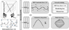 |
Fig. 1 Framework of the proposed NIM for small body shape modeling. The network employs an MLP architecture to learn neural fields that encode the SDF and color information, using volumetric rendering to integrate these properties and ultimately reconstruct the target shape models (Sect. 2.1). This method relies on a limited number of images while leveraging multi-scale deformation grids (Sect. 2.2) and explicit SDF constraints (Sect. 2.3) to reconstruct high-resolution shape models. |
2 Methodology
Figure 1 illustrates the framework of the proposed NIM for the global shape modeling of small bodies, designed to achieve detailed reconstruction using only a sparse set of images. This section begins with an introduction to the NIM in Sect. 2.1. Then, we describe the multi-scale deformable grids to provide neighboring information with flexible representations in Sect. 2.2 and present the explicit 3D point-based supervision used to improve the surface geometry in Sect. 2.3. Finally, Sect. 2.4 describes the details of the network training.
2.1 Small body shape modeling with NIM
First, the SfM technique is used to recover the poses of the input images and generate a sparse point cloud of the body (Schonberger & Frahm 2016; Chen et al. 2024a). The NIM then samples points along rays originating from the camera center (O) and passing through randomly selected pixels on the image, with the sparse point cloud defining the sampling boundary, as shown in Fig. 1a. The positions of these sampled points (x ∈ ℝ3), along with their view directions (v ∈  ), which correspond to the ray directions, serve as inputs to the method. To represent the small body’s surface, the NIM utilizes the signed distance function (SDF), which defines the distance of each point from the nearest surface (Mildenhall et al. 2021; Chen et al. 2024a). The surface (S) is then extracted as the zero-level set of this function. The NIM encodes S along with the object’s appearance (or color) (C) as a signed distance field fs and a radiance field fc (Mildenhall et al. 2021). These fields are parameterized using fully connected neural networks, specifically multi-layer perceptrons (MLPs) (Goodfellow et al. 2016), as illustrated in Fig. 2.
fs maps a x to its signed distance d ∈ ℝ,
 (1)
(1)
and fc encodes the color c ∈ ℝ3 associated with a point x and its v,
 (2)
(2)
The color of each selected pixel is determined through volume rendering, where the accumulated radiance along the camera ray is computed by integrating the volume density (σ) and c contributions from sampled points (Mildenhall et al. 2021),
 (3)
(3)
where N denotes the total number of points sampled along the ray; Δtj represents the spacing between consecutive samples j and j + 1; Ti represents the accumulated transmittance of sample i, computed as the exponential attenuation of the integrated σj over Δtj for all sampled points preceding point i (Mildenhall et al. 2021; Wang et al. 2021).
To provide accurate surface constraints for volume rendering optimization, the NIM applies a logistic sigmoid function to the predicted d from fs to derive σ (Wang et al. 2022). Once the volumetric representation is established through training, the final shape model of small bodies is extracted from the density field using the marching cubes algorithm (Mildenhall et al. 2021). This algorithm converts the density field into a mesh by detecting the surface where the density reaches a predefined threshold, which is typically equal to zero for SDF-based methods (Wang et al. 2021).
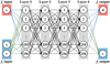 |
Fig. 2 Architecture of the MLP used in the proposed NIM, consisting of four layers with 256 neurons each. Each neuron in one layer is linked to every neuron in the next layer. The same network structure is used independently for fs and fc, but they do not share weights. |
2.2 Multi-resolution deformable grids
The input x serves as the key basis for learning the geometric structure of the object. Directly feeding x into the MLP introduces a learning bias, where the network predominantly captures low-frequency components, making it less effective in recovering fine geometric details (Mildenhall et al. 2021). This phenomenon arises due to the spectral bias of deep networks, which inherently prioritize smooth variations over high-frequency signals (Rahaman et al. 2019; Chen et al. 2022). To mitigate this limitation, positional encoding (PE) is commonly employed in NIMs to enrich the input representation by mapping x into a higher-dimensional space using sinusoidal functions at different frequency bands (Tancik et al. 2020),
 (4)
(4)
where n is usually set to 8.
However, the surface of Ryugu, like many other asteroids such as Itokawa and Bennu, exhibits pronounced roughness, characterized by high-frequency topographic features such as small-scale debris, regolith distributions, and irregularly shaped boulders (Tancredi et al. 2015; Michikami et al. 2019; Walsh et al. 2019). While PE enhances the network’s capability to model high-frequency details, it processes each x independently, struggling to effectively capture spatial correlations among neighboring features (Chen et al. 2024a). This limitation hinders the network’s ability to leverage local interactions, which often provide crucial geometric cues for reconstructing surface morphology. As an alternative, multi-resolution hash encoding introduces a hierarchical pyramid grid, assigning learnable encoding features to each vertex of the grid containing x (Müller et al. 2022; Chen et al. 2024c). Given that voxel grids are uniformly distributed in 3D space (as shown in Fig. 3a), they may lack the flexibility to capture the diverse topological features of asteroids. For instance, in the case of Ryugu, whose highly anisotropic terrain ranges from smooth regolith patches to dense boulder fields, this would require an encoding scheme that is able to dynamically adapt to these variations (Cai et al. 2023).
In the present work, we have used multi-resolution deformable grids to adaptively partition the 3D scene. To achieve this, we maintained a learnable 3D position at each vertex, rather than a hash-encoding feature vector. Initially, these vertex positions were uniformly distributed. During the training, they were dynamically adjusted by optimizing the loss function (as described in Sect. 2.4), which penalizes discrepancies between the vertex positions and the underlying surface geometry. This process progressively guides the vertices toward the surface features (as illustrated in Fig. 3b). This adaptivity allows the grid structure to conform to high-frequency terrain details, contributing to a more accurate representation of intricate surface morphology and fine geometric structures. Furthermore, asteroid surfaces often exhibit complex and multi-scale topographical variations, encompassing diverse features such as craters and boulders of varying sizes (Lauretta et al. 2019; Sugita et al. 2019; Michikami et al. 2019). The grid resolution was established at an eight-level hierarchical structure, consistent with multi-resolution hash encoding (Müller et al. 2022). This multi-resolution design enables the model to allocate encoding capacity dynamically across spatial frequencies, improving its ability to represent both finer details and large-scale geometric variations.
Applying a standard PE to each vertex (xl ∈ ℝ3) at every grid level (l) would result in a large-dimensional embedding. Specifically, with eight grid levels, a standard PE maps each three-dimensional xl to 48 dimensions. Since each level contains eight vertices, this results in a 384-dimensional representation per level. Consequently, for all 64 vertices in the multi-resolution deformable grids, the total embedding dimension reaches 3072.
To address this high dimensionality, a hierarchical PE is employed to transform the vertices:
 (5)
(5)
where each xl is mapped to six dimensions. As a result, at eight grid levels, the representation is reduced to 48 dimensions per level and all grid voxels collectively form a 384-dimensional embedding.
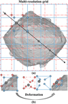 |
Fig. 3 Schematic of multi-resolution deformable grids, displayed in two dimensions with two levels of resolution: (a) depicts the uniformly subdivided grids, while (b) illustrates the deformation process, where vertices adjust their positions from a uniform distribution to a more adaptive arrangement. |
2.3 Explicit 3D point-based supervision
The NIM typically optimizes surface geometry using a rendering loss, which implicitly minimizes the discrepancy between images rendered from the 3D scene and real observations (Wang et al. 2021; Chen et al. 2024a),
 (6)
(6)
where M indicates the batch size of rays emitted from the camera center. Also, Ĉi and Ci denote the rendered and real pixel colors, respectively.
The sparse 3D points (p) generated by the SfM technique could act as crucial geometric priors for small bodies, as they are expected to align with the object’s surface. Each point inherently encodes a known surface location, where the SDF is zero, making them valuable for constraining shape reconstruction. However, despite their geometric significance, NIMs typically use p in a limited manner, primarily to delineate scene boundaries and constrain the sampling range. This prevents the network from allocating unnecessary capacity to regions outside the object, while overlooking the fact that these sparse points lie directly on the target surface. They can provide explicit supervision to refine the learned representation, rather than serving merely as sampling constraints (Fu et al. 2022).
To better leverage these 3D sparse points p, we introduce an SDF loss that explicitly supervises the signed distance field, fs, which estimates the signed distance of spatial points in the 3D scene to the surface of the body and is essential for optimizing the surface geometry. Since the points, p, are on the surface, their ground truth SDF value is
 (7)
(7)
We enforce this constraint by penalizing deviations between the predicted SDF value f̂s(p) and the ground truth fs(p) using an l1 loss. The SDF loss is defined as:
 (8)
(8)
where Q is the number of 3D points. f̂s(pi) and fs(pi) are the predicted and ground true SDF values at point pi. Given fs(pi) = 0 for surface points, the loss is simplified to
 (9)
(9)
This loss ensures that the predicted SDF values at surface points are close to zero, effectively aligning the learned geometry with the true surface. When processing a sparse set of images, the MVS techniques can efficiently generate a denser 3D point cloud by leveraging depth consistency across multiple viewpoints, refining the coarse reconstruction obtained from SfM (Schonberger & Frahm 2016). This study uses these dense points to provide explicit geometric supervision, enhancing the accuracy of fine-scale shape modeling for small bodies, which often exhibit irregular topographies.
2.4 Network training details
In addition to employing the loss terms lc and lsd f, which respectively minimize color discrepancies and provide explicit supervision using SfM-MVS derived 3D points (as introduced in Sect. 2.3), we impose an Eikonal loss term to regularize the field fs and encourage a valid SDF representation during training (Gropp et al. 2020). This loss enforces the Eikonal constraint that the gradient magnitude ||∇fs||2 approximates one, ensuring the SDF maintains a unit-speed distance field critical for accurate surface reconstruction (Gropp et al. 2020; Wang et al. 2021). The Eikonal loss is defined as:
 (10)
(10)
where f̂s(xi, j) is the predicted SDF value at point xi, j, ∇ f̂s(xi, j) is its gradient.
Then, the final loss function is formulated as:
 (11)
(11)
where w is the weight for leik, which is set to 0.1 in our experiment. Besides, the network is trained for 300 k iterations with a batch size of M = 512 rays per iteration and an initial learning rate of 0.0005. Each ray samples N = 128 points, consisting of 64 uniformly distributed along the ray and 64 adaptively sampled near the surface. The eight hierarchical deformable grids are structured with subdivisions increasing from 16 to 152, following an exponential growth pattern to capture geometric structures at multiple levels of detail. To ensure the MVS-derived points maintain high accuracy, we use only those with a reprojection error of no greater than 1 pixel.
3 Image data and results
3.1 Image data
High-resolution images captured remotely by the Optical Navigation Camera Telescope (ONC-T) can be used for shape reconstruction of Ryugu (Watanabe et al. 2017). The “Box-A” operations, conducted at an altitude of ∼20 km above the sub-Earth point (SEP), are aimed at performing a global mapping procedure using the ONC-T. In contrast, the “Box-C” operations are carried out at a lower altitude to observe the surface of the target closely. To test the performance of the proposed NIM at different altitudes, we selected two sets of images from both operations: 70 images from Box-A, with a resolution of ∼2.2 m, and 61 images from Box-C, with a resolution ranging from about 0.6 to 0.7 m. These sets were used to derive two different resolution shape models of Ryugu. The centered latitude of all selected images from the Box-A operation is approximately fixed near the equator at −8∘. Among the images from Box-C, 43 have center latitudes within ±10∘, nine are between 12∘ ∼ 16∘, while another nine are between −38∘ ∼−47∘. The positioning of these images relative to Ryugu was recovered using the SfM method (Schonberger & Frahm 2016; Chen et al. 2024a) and referenced to the Ryugu body-fixed frame as used in Watanabe et al. (2019). Figure 4a illustrates the spatial distribution of camera frusta for the selected images. Figure 4b displays example images from both operations, illustrating variations in Ryugu’s apparent size and surface details due to differences in camera distances and viewing angles.
3.2 Reconstruction results
Figure 5 illustrates the reconstructed Ryugu shape models generated by the proposed method using two distinct image sets. The figure showcases six-sided views for each model, offering a comprehensive visual comparison. The method effectively accommodates image sets with varying resolutions, enabling the recovery of detailed surface terrain features, such as differently shaped craters and boulders. The enlarged local areas in the right column of Fig. 5 demonstrate that more details become retrievable as the image resolution increases from Box-A to Box-C operations.
Figure 6 presents the reconstruction performance of the proposed method in capturing various boulders using the BoxC images. Figure 6a focuses on the reconstruction of smallscale boulders in the polar region. Our method effectively retrieves these features with higher fidelity, capturing intricate surface details. However, due to the limited camera coverage of the ONC-T in the polar region, the SfM-MVS method (Watanabe et al. 2019) struggles to obtain sufficient data points for a complete shape model. Consequently, the method needs to interpolate or extrapolate data to fill these gaps, leading to overly smoothed-out surfaces and a loss of fine geometric features. Figures 6b and 6c further depict two large-scale, irregularly shaped boulders. Our model exhibits a more continuous and well-defined surface representation, characterized by a dense vertex distribution that more faithfully follows the boulders’ natural contours. In contrast, the SfM-MVS method faces challenges in terms of accurately reconstructing these complex geometries. Due to the sparse distribution of reconstructed vertices in these regions, the resulting shape appears fragmented and lacks continuity. Additionally, the synthetic images further emphasize these discrepancies, demonstrating that our model is better equipped to capture the detailed morphology of boulders, including sharp edges and subtle topographical variations, thereby improving the overall reconstruction performance.
In addition, Table 1 provides a quantitative comparison of the volumes and surface areas of existing released Ryugu shape models and those derived using the proposed NIM. Compared to the previous NIM (Chen et al. 2024a), the proposed NIM yields shape models with volumes and surface areas that are more closely aligned with the SfM-MVS reference model (Watanabe et al. 2019). Notably, the SfM-MVS model reports a volume of 0.3774 km3 and a surface area of 2.7865 km2, which serves as a benchmark for evaluating the accuracy of other models. Among the models derived using the previous NIM (Chen et al. 2024a), the Box-A-based reconstruction shows a 0.21% volume increase and a 1.26% larger surface area compared to the SfM-MVS model. The Box-C-based reconstruction further deviates, with a 0.48% larger volume and a 2.16% larger surface area. In contrast, the proposed NIM improves the agreement with the reference model. Our Box-A-based version achieves a closer volume estimate (0.3768 km3, a −0.16% deviation) and surface area (2.7749 km2, a −0.42% deviation) relative to the SfM-MVS model. The Box-C-derived model from the proposed NIM continues this trend, with a volume of 0.3779 km3 and a surface area of 2.8152 km2, reducing discrepancies while achieving higher resolution. Overall, these results demonstrate that our method significantly improves the accuracy of shape modeling, particularly when using higher-resolution Box-C images, achieving the closest alignment with the benchmark SfM-MVS model.
Comparison of the volume and surface area with existing released Ryugu shape models.
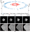 |
Fig. 4 Two image sets used to derive the Ryugu shape models. (a) shows the spatial distribution of camera frusta corresponding to images from the Box-A and Box-C operations. (b) eight example images, with the top row (1–4) corresponding to Box-A and showing a global view of Ryugu, while the bottom row (5–8) corresponds to Box-C and provides detailed close-up views of the surface. Their spatial locations are indicated in (a). |
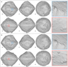 |
Fig. 5 Six views of Ryugu shape models derived using the proposed method from two image sets: (a) images from Box-A and (b) images from Box-C. The right column displays the local regions marked by the blue and pink boxes in the left column. |
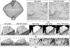 |
Fig. 6 Comparison of reconstruction performance on various boulders in three local areas: (a) our shape model and the SfM-MVS model (Watanabe et al. 2019) in the polar region. (b) and (c) our shape model, the SfM-MVS model, and corresponding synthetic images for two irregularly shaped boulders. The real image for (b) is hyb2_onc_20181030_063616_tvf_12c and for (c) it is hyb2_onc_20180720_105527_tvf_12c. |
4 Discussion
4.1 Accuracy analysis for the NIM
In this section, we analyze the accuracy of the NIMs proposed in this study and Chen et al. (2024a). The reference model derived from the SfM-MVS method utilized 124 images from the Box-C observation (∼6.5 km above the SEP) and 90 images from the Mid-Altitude observation (∼5.1 km above the SEP) to construct the Ryugu model (Watanabe et al. 2019). In particular, we examine the NIM-derived models using the Box-C image set.
4.1.1 Comparison of synthetic images
To assess the reconstruction performance of boulders, we compare real images with synthetic images generated from the SfM-MVS method, as well as NIMs proposed by Chen et al. (2024a) and this study, as shown in Fig. 7. For a more comprehensive comparison, additional examples are presented in Appendix A. The synthetic images are computed using NAIF’s SPICE toolkit (version N0067) (Acton 1996; Acton et al. 2018) and are based on the real images’ acquisition time, ephemeris data for Hayabusa2, the ONC-T’s nominal pointing and camera parameters, ephemeris data and a rotational model for Ryugu and, of course, different shape models1.
The synthetic images generated from the NIM model derived by Chen et al. (2024a) exhibit noticeable high-frequency artifacts, leading to distortions in the reconstructed surface and irregularities in the representation of boulders. These artifacts introduce a rough, unrealistic texture that deviates from the surface features observed in the real images. While the SfM-MVS method effectively reconstructs the global shape of Ryugu, it lacks the fidelity to capture small-scale terrain features. Despite using a large number of images, 3.5 times as many as our method, it produces overly smooth reconstructions that blur fine details, making individual boulders appear indistinct. By comparison, the proposed NIM model demonstrates better performance in preserving surface features. The synthetic images generated from our model exhibit a higher degree of consistency with the real ONC-T images, accurately capturing the shapes and distribution of boulders across various scales. Overall, our approach provides improved geometric fidelity, ensuring a more realistic representation of the asteroid’s terrain.
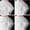 |
Fig. 7 Comparison of ONC-T images (hyb2_onc_20180720_071230_tvf_12c) with synthetic images from the SfM-MVS model (Watanabe et al. 2019), and the NIM models derived from Chen et al. (2024a) and the proposed method. |
4.1.2 Absolute error comparison with the SfM-MVS model
Furthermore, we evaluate the absolute error between the NIM-derived models and the SfM-MVS model (Watanabe et al. 2019), as shown in Fig. 8. The error distributions reveal that the most significant discrepancies occur in the polar regions, where limited observational coverage provides fewer constraints for the SfM-MVS method. Figure 8a presents the error map of Chen et al. (2024a), showing extensive high error regions, particularly in areas with large irregularly shaped boulders. In contrast, Fig. 8b demonstrates that the proposed NIM reduces these discrepancies, resulting in a lower error distribution across the surface.
To quantitatively assess these differences, in Table 2, we compare the accuracy of the NIMs at different absolute error thresholds. The accuracy is defined as the percentage of vertices in the reconstructed shape model whose absolute error, relative to the SfM-MVS reference model (Watanabe et al. 2019), falls within specified thresholds, such as ≤ 1 m and ≤ 2 m. This is determined by computing the Euclidean distance from each vertex in the NIM-derived model to its nearest corresponding point on the SfM-MVS model and then calculating the proportion of vertices that satisfy each threshold.
The proposed NIM achieves a 95.48% accuracy at the 2 meter threshold, surpassing the 87.69% accuracy of Chen et al. (2024a), demonstrating enhanced reliability in fine-scale reconstruction. The advantage becomes even more pronounced at the 1 meter threshold, where our model retains 80.71% accuracy, compared to only 57.10% for Chen et al. (2024a). Across all thresholds, the proposed method consistently outperforms the NIM proposed by Chen et al. (2024a), highlighting its ability to generate a more precise shape model, while utilizing only a small set of images.
Accuracy comparison of NIMs with respect to the SfM-MVS method (Watanabe et al. 2019) at different absolute error thresholds.
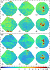 |
Fig. 8 Absolute errors between models derived using the NIMs and the SfM-MVS method (Watanabe et al. 2019): (a) results from Chen et al. (2024a); (b) results from the proposed NIM. The values represented by colors are mapped using a 0.4 power transformation to enhance the visual contrast. |
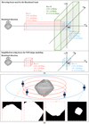 |
Fig. 9 Schematic of the spacecraft hovering (or orbiting) the target, using Ryugu as an example: (a) spacecraft hovering boxes defined by the Hayabusa2 team and our simplified operation mode; (b) orbits of spacecraft around the target in the Ryugu body-fixed frame. |
4.2 Suggestions to future mission planning
While the proposed NIM uses only a small number of images, it effectively reconstructs boulders of varying sizes, from small-scale features to large, irregularly shaped formations. This advantage allows for the simplification of mission planning during the proximity phase for global shape modeling. As shown in Fig. 9, the Hayabusa2 team defined three regions for spacecraft operations above Ryugu (Saiki et al. 2022): Box-A spans 1 km × 1 km horizontally (X and Y) and extends up to 5 km vertically (Z), with its center corresponding to the Home Position (HP) at an altitude of ∼20 km. Box-B shares the same altitude as Box-A, but it permits a wider range of 10 km in both X and Y directions. Box-C mirrors Box-A’s horizontal dimensions but allows descent to 5 km above the asteroid surface along the Z axis. The images obtained from Box-A comprehensively depict its appearance. Considering Ryugu’s rotation period of ∼7.6 hours (Watanabe et al. 2019), acquiring images for NIM-based shape modeling is feasible within a single day (and even in as little as 7.6 hours). For detailed global shape modeling, we propose carrying out a new Box-C operation to hover the spacecraft above Ryugu. The Z direction range is narrowed from 5–17.5 km to 5–7 km to ensure similar image resolutions. As images captured from Box-C only partially cover the target, multiple hovering points along the Y direction are recommended to fully capture the appearance of the target. Figure 9b depicts the suggested orbits of the spacecraft relative to the target in Ryugu’s body-fixed frame.
5 Conclusions
This paper presents an improved NIM for high-resolution shape modeling of Ryugu, which is covered in boulders and exhibits a varied surface, using a sparse image set. To accurately reconstruct the geometric structures of various boulders, we have introduced multi-scale deformable grids to flexibly learn neighboring information with different receptive fields. We used 3D points derived from the SfM-MVS method, where the SDF is zero, to provide explicit supervision, thereby enhancing the accuracy of surface reconstruction. We demonstrate that the proposed NIM can reliably reconstruct the Ryugu shape models from two image sets with different resolutions, yielding consistent volumes and surface areas compared to the SfM-MVS model, particularly when utilizing images from the Box-C set. Our method effectively reconstructs the small-scale boulders and the large-scale, irregularly shaped boulders. Furthermore, we can retrieve terrain features in the polar regions, despite the limited coverage provided by the ONC-T. Due to the relaxed image requirements, this method offers the possibility of simplifying mission planning with respect to image acquisition for global shape modeling.
While our method requires only a small number of images, these images must have a similar resolution when we are looking to derive a shape model. However, for some small bodies, such as Phobos, there may be insufficient images with a similar enough resolution to cover them completely. In the future, we will investigate the high-quality reconstruction of small bodies using images of varying resolution.
Acknowledgements
Part of this work was supported by the China Scholarship Council (CSC) under Grants 202006260004. This research was supported by the International Space Science Institute (ISSI) in Bern and Beijing, through ISSI/ISSI-BJ International Team project ‘Timing and Processes of Planetesimal Formation and Evolution’ (ISSI Team project #561; ISSI-BJ Team project #54).
Appendix A Extended comparison of synthetic images
Figure A.1 presents a comparison of synthetic images generated by the SfM-MVS model, the NIM models from Chen et al. (2024a), and the proposed method, using the ONC-T image (hyb2_onc_20181030_094954_tvf_12c) as the real image.
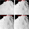 |
Fig. A.1 Comparison of ONC-T images (hyb2_onc_20181030_094954_tvf_12c) with synthetic images from the SfM-MVS model (Watanabe et al. 2019), and the NIM models derived from Chen et al. (2024a) and the proposed method. |
References
- Acton, C. H. 1996, Planet. Space Sci., 44, 65 [Google Scholar]
- Acton, C., Bachman, N., Semenov, B., & Wright, E. 2018, Planet. Space Sci., 150, 9 [Google Scholar]
- Al Asad, M., Philpott, L., Johnson, C., et al. 2021, Planet. Sci. J., 2, 82 [NASA ADS] [CrossRef] [Google Scholar]
- Cai, B., Huang, J., Jia, R., Lv, C., & Fu, H. 2023, in the Proceedings of the IEEE/CVF Conference on Computer Vision and Pattern Recognition, 8476 [Google Scholar]
- Chen, H., Hu, X., Gläser, P., et al. 2022, IEEE J. Sel. Top. Appl. Earth Obs. Remote Sens., 15, 9398 [Google Scholar]
- Chen, M., Huang, X., Yan, J., Lei, Z., & Barriot, J. P. 2023, Icarus, 401, 115566 [NASA ADS] [CrossRef] [Google Scholar]
- Chen, H., Hu, X., Willner, K., et al. 2024a, ISPRS J. Photogramm. Remote Sens., 212, 122 [Google Scholar]
- Chen, M., Yan, J., Huang, X., et al. 2024b, A&A, 684, A89 [NASA ADS] [CrossRef] [EDP Sciences] [Google Scholar]
- Chen, S., Wu, B., Li, H., Li, Z., & Liu, Y. 2024c, A&A, 687, A278 [NASA ADS] [CrossRef] [EDP Sciences] [Google Scholar]
- Daly, R. T., Ernst, C. M., Gaskell, R. W., Barnouin, O. S., & Thomas, P. C. 2018, Lunar Planet. Sci. Conf., 1053 [Google Scholar]
- Fu, Q., Xu, Q., Ong, Y. S., & Tao, W. 2022, Adv. Neural Inform. Process. Syst., 35, 3403 [Google Scholar]
- Gaskell, R., Barnouin-Jha, O., Scheeres, D. J., et al. 2008, Meteorit. Planet. Sci., 43, 1049 [NASA ADS] [CrossRef] [Google Scholar]
- Gaskell, R., Barnouin, O., Daly, M., et al. 2023, Planet. Sci. J., 4, 63 [NASA ADS] [CrossRef] [Google Scholar]
- Giese, B., Neukum, G., Roatsch, T., Denk, T., & Porco, C. C. 2006, Planet. Space Sci., 54, 1156 [NASA ADS] [CrossRef] [Google Scholar]
- Goodfellow, I., Bengio, Y., & Courville, A. 2016, Deep Learning (Cambridge: MIT press) [Google Scholar]
- Gropp, A., Yariv, L., Haim, N., Atzmon, M., & Lipman, Y. 2020, Proc. Int. Conf. Mach. Learn., 119, 3789 [Google Scholar]
- Jorda, L., Gaskell, R., Capanna, C., et al. 2016, Icarus, 277, 257 [Google Scholar]
- Lauretta, D., DellaGiustina, D., Bennett, C., et al. 2019, Nature, 568, 55 [NASA ADS] [CrossRef] [Google Scholar]
- Michikami, T., Honda, C., Miyamoto, H., et al. 2019, Icarus, 331, 179 [NASA ADS] [CrossRef] [Google Scholar]
- Mildenhall, B., Srinivasan, P. P., Tancik, M., et al. 2021, Commun. ACM, 65, 99 [Google Scholar]
- Müller, T., Ďurech, J., Ishiguro, M., et al. 2017, A&A, 599, A103 [NASA ADS] [CrossRef] [EDP Sciences] [Google Scholar]
- Müller, T., Evans, A., Schied, C., & Keller, A. 2022, ACM Trans. Graph., 41, 1 [Google Scholar]
- Oberst, J., Gwinner, K., & Preusker, F. 2014, in Encyclopedia of the Solar System (Amsterdam: Elsevier), 1223 [CrossRef] [Google Scholar]
- Palmer, E. E., Gaskell, R., Daly, M. G., et al. 2022, Planet. Sci. J., 3, 102 [NASA ADS] [CrossRef] [Google Scholar]
- Park, R., Vaughan, A., Konopliv, A., et al. 2019, Icarus, 319, 812 [NASA ADS] [CrossRef] [Google Scholar]
- Preusker, F., Scholten, F., Matz, K.-D., et al. 2015, A&A, 583, A33 [NASA ADS] [CrossRef] [EDP Sciences] [Google Scholar]
- Preusker, F., Scholten, F., Matz, K.-D., et al. 2016, Lunar Planet Sci. Conf., 1954 [Google Scholar]
- Rahaman, N., Baratin, A., Arpit, D., et al. 2019, Int. Conf. Mach. Learn., 975301 [Google Scholar]
- Remondino, F., Karami, A., Yan, Z., et al. 2023, Remote Sens., 15, 3585 [Google Scholar]
- Saiki, T., Takei, Y., Fujii, A., et al. 2022, in Hayabusa2 Asteroid Sample Return Mission (Elsevier), 113 [CrossRef] [Google Scholar]
- Schonberger, J. L., & Frahm, J.-M. 2016, in the Proceedings of the IEEE conference on computer vision and pattern recognition, 4104 [Google Scholar]
- Sugita, S., Honda, R., Morota, T., et al. 2019, Science, 364, eaaw0422 [Google Scholar]
- Tancik, M., Srinivasan, P., Mildenhall, B., et al. 2020, Adv. Neural Inform. Process. Syst., 33, 7537 [Google Scholar]
- Tancredi, G., Roland, S., & Bruzzone, S. 2015, Icarus, 247, 279 [NASA ADS] [CrossRef] [Google Scholar]
- Walsh, K., Jawin, E., Ballouz, R.-L., et al. 2019, Nat. Geosci., 12, 242 [NASA ADS] [CrossRef] [Google Scholar]
- Wang, P., Liu, L., Liu, Y., et al. 2021, arXiv eprint [arXiv:2106.10689] [Google Scholar]
- Wang, Y., Skorokhodov, I., & Wonka, P. 2022, Adv. Inform. Process. Syst., 35, 1966 [Google Scholar]
- Watanabe, S.-i., Tsuda, Y., Yoshikawa, M., et al. 2017, Space Sci. Rev., 208, 3 [Google Scholar]
- Watanabe, S., Hirabayashi, M., Hirata, N., et al. 2019, Science, 364, 268 [NASA ADS] [Google Scholar]
- Willner, K., Oberst, J., Hussmann, H., et al. 2010, Earth Planet. Sci. Lett., 294, 541 [Google Scholar]
The kernels that were used are collected in the Hayabusa2 mission’s metakernel hyb2_v03.tm.
All Tables
Comparison of the volume and surface area with existing released Ryugu shape models.
Accuracy comparison of NIMs with respect to the SfM-MVS method (Watanabe et al. 2019) at different absolute error thresholds.
All Figures
|
Fig. 1 Framework of the proposed NIM for small body shape modeling. The network employs an MLP architecture to learn neural fields that encode the SDF and color information, using volumetric rendering to integrate these properties and ultimately reconstruct the target shape models (Sect. 2.1). This method relies on a limited number of images while leveraging multi-scale deformation grids (Sect. 2.2) and explicit SDF constraints (Sect. 2.3) to reconstruct high-resolution shape models. |
| In the text | |
|
Fig. 2 Architecture of the MLP used in the proposed NIM, consisting of four layers with 256 neurons each. Each neuron in one layer is linked to every neuron in the next layer. The same network structure is used independently for fs and fc, but they do not share weights. |
| In the text | |
|
Fig. 3 Schematic of multi-resolution deformable grids, displayed in two dimensions with two levels of resolution: (a) depicts the uniformly subdivided grids, while (b) illustrates the deformation process, where vertices adjust their positions from a uniform distribution to a more adaptive arrangement. |
| In the text | |
|
Fig. 4 Two image sets used to derive the Ryugu shape models. (a) shows the spatial distribution of camera frusta corresponding to images from the Box-A and Box-C operations. (b) eight example images, with the top row (1–4) corresponding to Box-A and showing a global view of Ryugu, while the bottom row (5–8) corresponds to Box-C and provides detailed close-up views of the surface. Their spatial locations are indicated in (a). |
| In the text | |
|
Fig. 5 Six views of Ryugu shape models derived using the proposed method from two image sets: (a) images from Box-A and (b) images from Box-C. The right column displays the local regions marked by the blue and pink boxes in the left column. |
| In the text | |
|
Fig. 6 Comparison of reconstruction performance on various boulders in three local areas: (a) our shape model and the SfM-MVS model (Watanabe et al. 2019) in the polar region. (b) and (c) our shape model, the SfM-MVS model, and corresponding synthetic images for two irregularly shaped boulders. The real image for (b) is hyb2_onc_20181030_063616_tvf_12c and for (c) it is hyb2_onc_20180720_105527_tvf_12c. |
| In the text | |
|
Fig. 7 Comparison of ONC-T images (hyb2_onc_20180720_071230_tvf_12c) with synthetic images from the SfM-MVS model (Watanabe et al. 2019), and the NIM models derived from Chen et al. (2024a) and the proposed method. |
| In the text | |
|
Fig. 8 Absolute errors between models derived using the NIMs and the SfM-MVS method (Watanabe et al. 2019): (a) results from Chen et al. (2024a); (b) results from the proposed NIM. The values represented by colors are mapped using a 0.4 power transformation to enhance the visual contrast. |
| In the text | |
|
Fig. 9 Schematic of the spacecraft hovering (or orbiting) the target, using Ryugu as an example: (a) spacecraft hovering boxes defined by the Hayabusa2 team and our simplified operation mode; (b) orbits of spacecraft around the target in the Ryugu body-fixed frame. |
| In the text | |
|
Fig. A.1 Comparison of ONC-T images (hyb2_onc_20181030_094954_tvf_12c) with synthetic images from the SfM-MVS model (Watanabe et al. 2019), and the NIM models derived from Chen et al. (2024a) and the proposed method. |
| In the text | |
Current usage metrics show cumulative count of Article Views (full-text article views including HTML views, PDF and ePub downloads, according to the available data) and Abstracts Views on Vision4Press platform.
Data correspond to usage on the plateform after 2015. The current usage metrics is available 48-96 hours after online publication and is updated daily on week days.
Initial download of the metrics may take a while.