| Issue |
A&A
Volume 684, April 2024
|
|
|---|---|---|
| Article Number | A85 | |
| Number of page(s) | 24 | |
| Section | Stellar structure and evolution | |
| DOI | https://doi.org/10.1051/0004-6361/202348133 | |
| Published online | 05 April 2024 | |
Stellar population astrophysics with the TNG
Abundance analysis of nearby red giants and red clump stars: Combining high-resolution spectroscopy and asteroseismology⋆,⋆⋆
1
Dipartimento di Fisica e Astronomia, Università di Padova, Vicolo dell’Osservatorio 2, 35122 Padova, Italy
e-mail: This email address is being protected from spambots. You need JavaScript enabled to view it.
2
INAF – Ossevatorio Astronomico di Padova, Vicolo dell’Osservatorio 5, 35122 Padova, Italy
e-mail: This email address is being protected from spambots. You need JavaScript enabled to view it.
3
INAF – Osservatorio di Astrofisica e Scienza dello Spazio, Via P. Gobetti 93/3, 40129 Bologna, Italy
4
Department of Physics and Astronomy, Università di Bologna, Via Zamboni 33, 40126 Bologna, Italy
5
INAF – Osservatorio Astrofisico di Arcetri, Largo Enrico Fermi, 5, 50125 Firenze, Italy
6
Fundación Galileo Galilei – INAF, Rambla José Ana Fernández Pérez 7, 38712 Breña Baja, Tenerife, Spain
7
INAF – Osservatorio Astronomico di Roma, Via Frascati 33, 00078 Monte Porzio Catone, Italy
8
INAF – Osservatorio Astrofisico di Catania, Via S. Sofia 78, 95123 Catania, Italy
Received:
2
October
2023
Accepted:
15
January
2024
Abstract
Context. Asteroseismology, a powerful approach for obtaining internal structure and stellar properties, requires surface temperature and chemical composition information to determine mass and age. High-resolution spectroscopy is a valuable technique for precise stellar parameters (including surface temperature) and for an analysis of the chemical composition.
Aims. We combine spectroscopic parameters with asteroseismology to test stellar models.
Methods. Using high-resolution optical and near-IR spectra from GIARPS at the Telescopio Nazionale Galileo, we conducted a detailed spectroscopic analysis of 16 stars that were photometrically selected to be on the red giant and red clump branch. Stellar parameters and chemical abundances for light elements (Li, C, N, and F), Fe peak, α and n-capture elements were derived using a combination of equivalent widths and spectral synthesis techniques based on atomic and molecular features. Ages were determined through asteroseismic scaling relations and were compared with ages based on chemical clocks, [Y/Mg] and [C/N].
Results. The spectroscopic parameters confirmed that the stars are part of the red giant branch and red clump. Two objects, HD 22045 and HD 24680, exhibit relatively high Li abundances, and HD 24680 might be a Li-rich giant resulting from mass transfer with an intermediate-mass companion that already underwent its asymptotic giant branch phase. The stellar parameters derived from scaling different sets of relations were consistent with each other. The values based on asteroseismology for the ages agree excellently with those derived from theoretical evolutionary tracks, but they disagree with ages derived from the chemical clocks [Y/Mg] and [C/N].
Key words: techniques: spectroscopic / stars: abundances / stars: evolution
Stellar parameters, abundances, and tables of equivalent widths for each of the stars are available at the CDS via anonymous ftp to cdsarc.cds.unistra.fr (130.79.128.5) or via https://cdsarc.cds.unistra.fr/viz-bin/cat/J/A+A/684/A85
Based on observations made with the Italian Telescopio Nazionale Galileo (TNG) operated on the island of La Palma by the Fundación Galileo Galilei of the INAF (Istituto Nazionale di Astrofisica) at the Spanish Observatorio del Roque de los Muchachos of the Instituto de Astrofisica de Canarias.
© The Authors 2024
 Open Access article, published by EDP Sciences, under the terms of the Creative Commons Attribution License (https://creativecommons.org/licenses/by/4.0), which permits unrestricted use, distribution, and reproduction in any medium, provided the original work is properly cited.
This article is published in open access under the Subscribe to Open model. This email address is being protected from spambots. You need JavaScript enabled to view it. to support open access publication.
1. Introduction
Galactic archaeology is the study of present-time stellar populations in the Milky Way to probe the physical processes that resulted in the formation and subsequent evolution of our Galaxy and its components. The study of the properties of stars, position, kinematics, and chemical composition provides key information about the manner and location of the star formation. In this context, the upcoming high-resolution high-multiplexing spectroscopic surveys WEAVE1, 4MOST2, SDSSV-MWM3, building upon previous surveys, such as APOGEE4, Gaia-ESO5, and GALAH6, combined with Gaia parallaxes and proper motions are expected to enable a major step forward in the next few years.
The determination of ages is a critical point in Galactic archaeology. Deriving ages is rather challenging because we lack observables that are uniquely sensitive to age alone (Soderblom 2010). Traditionally, stellar ages are obtained through isochrone fitting on the basis of their atmospheric parameters (Teff, log(g), and chemical composition). While this approach proves highly effective for members of stellar clusters, it is limited when applied to individual field stars because the properties are inherently degenerate.
An alternative approach is to rely on information resulting from asteroseismological studies. Asteroseismology, the study of stellar oscillations, is a powerful technique for probing the internal structure and properties of stars. Through the analysis of the observed frequencies, amplitudes, and mode patterns of stellar oscillations, asteroseismology allows us to unravel fundamental information about stellar interiors (see Hekker & Christensen-Dalsgaard 2017, and references therein). Scaling relations, which link asteroseismic observables and the fundamental properties of stars, are used to estimate stellar masses, radii, and surface gravity. They also require as input information about the stellar surface temperature, and, in some formulations of these relations, information about the chemical composition (e.g. Kjeldsen & Bedding 1995; Guggenberger et al. 2016).
It is therefore a powerful tool for obtaining stellar properties, ages, and internal stellar structures when asteroseismology is complemented with high-resolution spectroscopy. This combination of techniques could also be used to test the reliability of theoretical models and probe the reliability of alternative approaches to age measurements (e.g. chemical clocks).
In this paper, we present the analysis of high-resolution optical and near-infrared (IR) spectroscopy for a sample of bright local red giant stars for which K2 data (Howell et al. 2014) are available. We compare quantities inferred from the spectra to those derived from asteroseimological data. In Sect. 2 we describe the sample selection along with the data we used for the analysis. Section 3 describes the procedure we followed to determine the stellar parameters and elemental abundances, including obtaining ages from asteroseismology and stellar tracks. A discussion of the results is given in Sect. 4, and a summary and conclusion are provided in Sect. 5.
2. Sample and observations
We wished to test the stellar evolutionary and asteroseismological models. It was therefore necessary to obtain good-quality photometric and spectroscopic data. We selected 16 bright red giant stars that were nearby and within the field of view of the K2 mission (Howell et al. 2014) to facilitate obtaining high-resolution spectroscopic data with a good signal-to-noise ratio. We also gathered high-precision photometric data for all the stars through the K2 mission. These were field stars and not part of any cluster, which hindered an accurate determination of their evolutionary stage. We used colour indices and Gaia information (Gaia Collaboration 2022) to estimate their evolutionary stage and select those that were most likely to be red clump or lower red giant branch (RGB) stars. We mainly concentrated on these because they are homogeneous type stars that are warm enough for a good estimation of the stellar parameters and abundances without having to worry about line crowding, as is seen in brighter giants at solar metallicity.
All the spectroscopic data used in this work were obtained using the 3.5 m Telescopio Nazionale Galileo (TNG) located in La Palma, Spain. Of its many instruments, TNG has two high-resolution spectrographs: HARPS-N7 (Cosentino et al. 2012) and GIANO (Oliva et al. 2012; Origlia et al. 2014). HARPS-N works in the optical, with a resolution of 115 000 and a wavelength coverage of 3800–6900 Å, whereas GIANO works in the IR, with a resolution of 50 000 and wavelength coverage of 0.97–2.4 μm, that is, YJHK. At the TNG, these two instruments can be used simultaneously in the GIARPS mode (Claudi et al. 2017). In this mode, every observation covers the optical as well as the IR wavelength regions. The log of the observations, together with information on the signal-to-noise ratio (S/N) reached with HARPS-N and GIANO, can be found in Table 1.
Observation log of the sample.
The data reduction of the optical spectra from HARPS-N, which includes flat-field and bias correction, spectral extraction, and wavelength calibration, was performed by the dedicated pipeline. For GIANO, the reduction was also performed with the offline version of the GOFIO reduction software (Rainer et al. 2018), and the telluric correction was performed using the spectra of telluric standards. Details of the procedure are described in Origlia et al. (2019). When the reduced spectra were obtained, we used the iSpec tool (Blanco-Cuaresma et al. 2014) to carry out continuum normalisation and radial velocity (RV) correction. For the continuum normalisation, we divided the observed spectrum by a fitted spline function. iSpec determines the RV by computing the cross-correlation function between the observed and synthetic spectra. Table 2 provides an overview of all the stars along with the estimated RV. Upon comparing our RV values with those of Gaia, we see an excellent agreement between the two, with a mean difference of 0.2 km s−1 and no trends, as shown in Fig. 1. Only one star (HD24680) shows a strong discrepancy in the RV along with a large error in the Gaia RV. This star is classified as an SB1 system (Gaia Collaboration 2022).
Stellar properties.
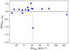 |
Fig. 1. Comparison of RV values obtained in this work (indicated by the suffix spec) and Gaia. The errors are the propagated uncertainties on both RVspec and RVGaia. |
To validate our results, we also analysed Arcturus. We obtained a high-resolution spectrum of Arcturus in the optical range from Hinkle et al. (2000) with a resolution R = 150 000 and S/N ∼ 1000. The spectrum was corrected for tellurics and was continuum normalised. The IR spectrum was obtained from Hinkle et al. (1995) with a wavelength coverage of 0.9–5.3 μm and a resolution R = 100 000.
3. Analysis
3.1. Stellar parameters
In order to perform a uniform analysis of all the stars, we started by determining the stellar parameters (Teff, log(g), [Fe/H], and ξmic) for all the stars in the sample and for Arcturus, which was used to assess the accuracy of our measurements. The stellar parameters were determined spectroscopically, with the standard approach of an excitation equilibrium of the iron lines, where Teff and ξmic were determined by minimising the trends of the Fe I abundance with respect to the excitation potential (EP) and reduced equivalent widths, respectively. The log(g) were derived using the ionisation equilibrium, where the difference in the abundances of Fe I and Fe II should be smaller than 1σ.
The initial guesses for temperature and log(g) were derived using a combination of photometry and isochrone fitting. We determined the colour temperature by averaging the temperatures obtained using the combination of photometric colours (B, V, J, K, G, GBP, and GRP) using calibrations from Mucciarelli & Bellazzini (2020) for Gaia DR2. For log(g), an initial guess was obtained by fitting an isochorone obtained from PARSEC8 (Bressan et al. 2012) with age = 0.5 Gyr and a metallicity of −0.1 dex. For the microturbulance, a constant value of 1.5 km s−1 was taken as the initial estimate. This is a rough approximation, but we recall that the parameters were determined spectroscopically, and the result is rather robust with respect to variations in the first-guess values.
The line list we adopted for the Fe transitions is reported in Table I.1 and is based on the line list in D’Orazi et al. (2015). The equivalent widths (EWs) were measured using ARES (Sousa et al. 2007). We removed any line with an EW smaller than 4σ of the fitting error and lines with EW > 150 mÅ. The assumptions adopted by ARES in the line fitting become less appropriate for strong lines, and moreover, strongly saturated lines are only poor indicators of the chemical abundance of the species from which they arise. Finally, we adopted the grid of Kurucz stellar atmospheres (Kurucz et al. 1992).
We performed the analysis using the abfind driver of MOOG (Sneden 1973) in its Python-wrapped version, pyMOOGi9). The values of the input stellar parameters were changed until the trends of Fe abundance with excitation potential, reduced EWs were flattened (within the errors), and the differences between Fe II and Fe I abundances were within the observational uncertainties. After the parameters were estimated using Fe, we refined them by repeating the whole process with the Ti lines given in Table I.2. The difference in parameters estimated using Fe and Ti was smaller than the uncertainties on the parameters (δ Teff = 50 K, δ log(g) = 0.1 dex and δ ξmic = 0.05 km s−1). The parameters we obtained for our sample are given in Table 3 with the colour-magnitude diagram (CMD) and Kiel diagram in Figs. 2 and 3, respectively.
Stellar properties (effective temperature, surface gravity, metallicity, and microturbulent velocity) for all the stars in the sample and Arcturus.
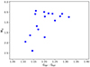 |
Fig. 2. Colour-magnitude diagram of the stars using Gaia magnitudes and parallaxes to compute the absolute magnitude MG. |
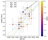 |
Fig. 3. Kiel diagram (Teff vs. log(g)) of the stars using stellar parameters from spectroscopic analysis with an overlay of metallicity. The three dashed lines represent the stellar isochrones with ages of 3 Gyr (blue), 5 Gyr (orange), and 7 Gyr (green), and a metallicity of −0.1 dex. |
Together with our sample, we performed an analysis of Arcturus. For Arcturus, we obtained an effective temperature of 4300 ± 70 K, log(g) of 1.66 ± 0.20 dex, [Fe/H] of −0.50 ± 0.10 dex and ξmic of 1.74 ± 0.08 km s−1. These values are consistent with the values obtained by Ramírez & Allende Prieto (2011).
Because our sample is homogeneous, the uncertainties on each of the parameters were very similar for all the stars. We adopted uniform uncertainties as follows: 100 K on Teff, 0.30 dex on log(g), 0.13 dex on [Fe/H]10, and 0.10 km s−1 on ξmic.
The comparison between the effective temperature obtained through photometric magnitudes and from spectroscopic analysis is shown in Fig. 4. Even though the two temperatures agree within the errors for some stars, for the whole sample, the mean difference is about 90 K and the standard deviation is 85 K, and the spectroscopic temperatures are higher. This offset could be due to the metallicity value of −0.1 dex that was assumed to calculate the photometric temperature, or to unaccounted reddening, which seems unlikely given the spatial distribution of the objects. In Figs. 5 and A.1, we compare our stellar parameters (labelled MOOG) with those available in the literature, APOGEE, LAMOST11, and Gaia. The literature values were taken from different studies, such as Massarotti et al. (2008), Koleva & Vazdekis (2012), Jofré et al. (2015), Feuillet et al. (2016), Brewer et al. (2016), Ghezzi et al. (2018), Deka-Szymankiewicz et al. (2018), and Abia et al. (2021), whereas the APOGEE and LAMOST values were taken from Jönsson et al. (2020) and Ting et al. (2018), respectively.
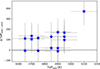 |
Fig. 4. Comparison of the effective temperature obtained from spectroscopy and photometry. |
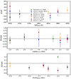 |
Fig. 5. Comparison of the stellar parameters (Teff, log(g), and [Fe/H]) with literature sources for Massarotti et al. (2008), Koleva & Vazdekis (2012), Jofré et al. (2015), Feuillet et al. (2016), Brewer et al. (2016), Ghezzi et al. (2018), Deka-Szymankiewicz et al. (2018), Abia et al. (2021). The black line represents the y = 0 line. In all three panels, each colour represents a specific study, as described in the legend. |
The data from large surveys, that is Gaia, APOGEE, and LAMOST mostly agree very well, as shown in Fig. A.1. On the other hand, the agreement is rather poor for Hardegree-Ullman et al. (2020), who reported the parameters derived with LAMOST spectra for four stars, especially for the temperature. We note, however, that their values are quite discrepant from the corresponding Gaia values.
Figure 5 shows the comparison with atmospheric parameters reported in small-scale studies. The temperature agrees well overall, with the exception of 78Cnc, where the value from Abia et al. (2021) shows a significantly higher temperature than is derived in our study. We have no explanation for this discrepancy, and we can only speculate that it might have to do with the different approach to the analysis adopted by the authors (automatic parameter determination based on the MATISSE algorithm), but we note that the value reported for the same object by Ghezzi et al. (2018) agrees well with ours.
We note, however, that some offsets between different studies are expected because different choices are made in the analysis (e.g. classes of model atmosphere, solar composition, line transition parameters, etc).
Considering the uncertainties on the MOOG parameters, these differences are not significant. The only significant difference we obtained was in the effective temperature of MOOG and Hardegree-Ullman et al. (2020). This difference is not reflected in the surface gravity or in the metallicity. When we assume that the Teff from Hardegree-Ullman et al. (2020) is correct, both the spectroscopic and photometric Teff would be incorrect. Given the photometric Teff was derived using different colour that indices, only extinction can introduce such a large deviation. However, with the stars located within the solar neighbourhood, the extinction is likely to be low, which was verified using Gaia DR3. This is further supported by the small deviations in the derived temperatures of different colour indices. We therefore assume that our parameters are more reliable than those of Hardegree-Ullman et al. (2020), which is supported by Gaia and other literature values.
3.2. Elemental abundances
In order to test the stellar evolutionary models, we focused our abundance analysis on elements that are particularly affected by evolution, such as carbon, nitrogen, oxygen, and lithium. Along with these, we also analysed some of the α- and Fe-peak elements to obtain a better understanding of the chemical signatures. Additionally, we derived the abundance of fluorine, which is rarely measured, and of yttrium, to determine the relations between age and the ratio of α to neutron capture element. For the analysis, we used two methods: spectral synthesis, and equivalent width. We used the abfind driver of pyMOOGi for the equivalent width method and the synth driver for the spectral synthesis with interpolated Kurucz atmosphere models.
3.2.1. Carbon, nitrogen, and oxygen
Because GIARPS data are available for all but one of the stars, we conducted separate analyses on the optical and the IR spectrum using the spectral synthesis method. The line list for the entire CNO analysis was generated using the Linemake12 tool (Placco et al. 2021). We refer to the paper for details on the sources of the parameters of the atomic and molecular transitions that are taken into account.
For carbon, we used the CH band at 4300 Å and one carbon high-excitation line at 5380 Å in the optical, and the CO band at 2.30 μm in the IR. Nitrogen was determined using the CN bands at 4100 Å and 1.5 μm in the optical and IR region, respectively. We estimated the oxygen abundance from the two forbidden lines at 6300 and 6363 Å in the optical and two OH bands at 1.5 and 1.6 μm in the IR region. We note that for one star (HD 78419), only the optical spectrum was available. For HD 97716, we were unable to measure the oxygen abundance from the OH molecular band as the band was exceedingly weak. Telluric contamination usually becomes prominent at longer wavelengths (about 6000 Å), with strong contamination in the IR region. As the two oxygen lines were located in the region affected by the tellurics, we visually inspected the two lines in all the stars and found no contamination. For confirmation, we examined the line-by-line scatter in the sample, with the understanding that a contaminated line would result in a vastly different oxygen abundance compared to the other line. We found the line-by-scatter to be between 0.07 to 0.13 dex, without a strong difference between the two lines in any of the stars. We therefore conclude that the lines were not affected by telluric contamination. The telluric contamination in the IR spectrum was modelled (as shown in Fig. H.1) and subtracted using the TelFit code (Gullikson et al. 2014). Figures 6 and 7 show the fitting of the two oxygen lines in the optical and IR, respectively. The fitting of the CH (optical) and CO (IR) bands is shown in Fig. F.1 and the fitting of the CN band (both optical and IR) is shown in Fig. F.2.
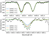 |
Fig. 6. Fitting of two oxygen lines at 6300 and 6363 Å in HD 5214. The observed spectrum is shown as black points, and the synthetic spectra of different oxygen abundances are shown in blue ([O/Fe] = 0.1 dex), orange ([O/Fe] = 0.2 dex), and green ([O/Fe] = 0.3 dex). A line-by-line scatter of 0.1 dex can be seen between the two. |
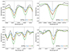 |
Fig. 7. Fitting of the OH band at 1.5 and 1.6 μm in HD 218330. The observed spectrum is shown in black, and the synthetic spectra of different oxygen abundances are shown in blue ([O/Fe] = 0.2 dex), orange ([O/Fe] = 0.4 dex), and green ([O/Fe] = 0.6 dex). The vertical dashed black line shows the OH lines considered for the abundance analysis. The best-fit line is shown in orange with O = 0.40 dex. |
From the abundances reported in Table 4, we found that the oxygen abundances obtained from the IR region were higher than those obtained from the optical atomic lines (see Fig. D.1). No such offset is seen in Arcturus. However, all the stars in our sample are considerably hotter and younger than Arcturus. Therefore, the absence of an offset in Arcturus might not exclude systematic differences from measurements based on an IR versus optical spectrum, intrinsic to the features analysed. As the OH band was weak and crowded, which is seen in Fig. C.1, we gave higher weight to the optical abundance because the atomic lines were relatively strong and well isolated. If the discrepancy between the two was within the errors of each other, we took the average, but if the discrepancy was larger, the optical abundance was assumed to be a better estimate and was used for the further analysis of carbon and nitrogen.
Abundances of carbon, nitrogen, and oxygen obtained from the optical and IR region.
For carbon, we again found that the abundance from the IR molecular band was larger than in the optical in the majority of the sample. However, the difference between the two is not as large as for oxygen. This discrepancy between the abundance of the optical and IR also extends to nitrogen, where the IR abundances are again larger than the optical. The high-excitation carbon lines did not agree with the abundance from the CH and CO bands either. The reason might be that only one high-excitation line is available within our spectral coverage. A similar offset is also found in Arcturus, where the high-excitation line returns an abundance that is higher by +0.3 dex than those obtained from the same CH and CO bands.
The abundances in Arcturus agree well for CNO. The difference between the optical and IR is δ[O/Fe] = 0.01 dex, δ[C/Fe] = 0.01 dex, and δ[N/Fe] = 0.05 dex, which are consistent within the errors.
After estimating the carbon abundance in the optical, we estimated the carbon isotopic ratio, that is, 12C/13C using the CH and 13CO (2–0) band-head in the optical and IR, respectively. Because the stars were observed in sub-optimal weather conditions, the 13CO molecular band at 2.34 μm had strong telluric contamination. Even after we modelled and subtracted these telluric lines using Telfit, many spectra had significant residuals, which increased the difficulty of obtaining a reliable measure of the isotopic ratios in most of the stars. We therefore first measured the isotopic ratio from the CH band in the optical and then used the 13CO band to refine the ratio. Figure 8 shows the fitting of the CO band in HD6432. We find values ranging between 15 and 6, as shown in Table 4.
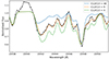 |
Fig. 8. Fitting of 13CO (2–0) band at 23442 Å in HD 6432 to estimate the carbon isotopic ratio. The observed spectrum is shown in black, and the synthetic spectra of varying isotopic ratios are shown in different colours. The best-fit carbon isotopic ratio is 9 (dashed orange line). |
3.2.2. Lithium
We used a spectral synthesis to probe the Li abundance using the line at 6707.78 Å. The line list for the synthesis was adopted from D’Orazi et al. (2015). With two exceptions (HD 24680 and HD 22045), we were only able to estimate upper limits on the Li abundance as the lines were weak. HD 24680 and HD 22045 both show relatively strong Li lines with A(Li) of 1.46 ± 0.20 and 0.65 ± 0.20 dex, respectively. Considering the errors, HD 24680 can be classified as a Li-rich giant (A(Li) > 1.5 dex, Brown et al. 1989). The lithium line of HD24680 is shown in Fig. 9, along with two other stars of the sample with similar stellar properties. The line is slightly blended with the neighbouring CN line. For Arcturus, we were unable to measure the Li abundance as the line was too weak.
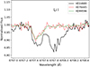 |
Fig. 9. Comparison of the Li line strength in HD 24680 (black), HD 76445 (red), and HD 99596 (green). The line in HD 24680 is slightly blended with a nearby CN line at 6707.45 Å. |
For the Li feature, LTE is a poor approximation (Lind et al. 2009), and in order to address this, we applied NLTE corrections, as prescribed by the INSPECT13 tool, which allows the user to estimate the NLTE correction on a line-by-line basis. In our sample, the correction ranged between 0.13 and 0.25 dex, and the NLTE abundance was higher than the LTE abundance. We note that the correction was not available for three stars because the lines were weak (small EWs). The Li abundances along with the NLTE corrections are reported in Table 5.
Abundances of α- and iron-peak elements, lithium, and flourine.
3.2.3. α and iron peak elements
We also derived the chemical abundances of a few α- and iron peak elements, namely Mg, Si, Ti, Ca, Cr, and Ni. For these elements, we used the equivalent width method based on measurements derived using ARES. The line list for each of the elements is given in Table I.3. Lines with large errors on the EWs or that resulted in discrepant abundances were manually checked using IRAF. The reliability of the abundances from individual lines were checked on a star-by-star basis. This was done by examining the difference in the line-by-line abundance with respect to the average abundance of that element in that particular star. By repeating this for all the stars, we can plot the mean of this difference along with its scatter, as shown in Fig. 10. The figure clearly shows that a number of lines show an offset (the mean is systematically higher or lower than 0), such as the Ca I lines at 6717 Å and 6462 Å. Some of the lines also show large scatter, for instance, the Cr II line at 5772 Å and the Ca I line at 6717 Å, with a standard deviation of 0.19 and 0.16, respectively. Offsets can be due to differences in the parameters of the transitions and/or an unaccounted-for contamination (i.e. blending with another line). When a line of interest is blended with a nearby line, ARES can find it difficult to accurately measure the EW. This results in the determination of an incorrect abundance. Therefore, we discarded any lines with a mean difference outside the range of −0.2 to 0.2 as the errors on the abundances range between 0.05 and 0.2 dex for different elements. On average, we measured 4, 4, 18, 26, 8, 8, and 5 lines for Mg, Si, Ca, Ti I, Ti II, Cr, and Ni, respectively. The abundances are listed in Table 5. Along with our sample, we also measured these elements in Arcturus. The abundances of all the elements except for Ni agree with Ramírez & Allende Prieto (2011) within their respective errors. The Ni abundance is lower by 0.1 dex in our analysis than in Ramírez & Allende Prieto (2011).
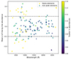 |
Fig. 10. Offset and scatter in the line-by-line abundance of α- and Fe-peak elements. The y-axis represents the mean of the standard deviation of the line-by-line abundance (average abundance from all the lines – abundance from the line). The colour represents the scatter of the standard deviation in different stars. The black line represents the offset limit of the mean, beyond which the line is discarded. |
3.2.4. Fluorine
Fluorine is a rather light element (Z = 9) in the periodic table. It lies next to nitrogen, oxygen, and neon. It is also a very poorly understood element in the context of stellar nucleosynthesis. This is the result of its relatively low abundance when compared to its neighbouring elements (it is lower by about four orders of magnitude than elements such as nitrogen and oxygen; Guerço et al. 2022), which hampers the detection of its lines in stellar spectra. Its content in stellar atmospheres is in fact only measurable through a limited number of very weak and often telluric-line contaminated transitions of the molecule HF. In addition to this, the possibility of fluorine formation in a variety of astrophysical sites makes it difficult to understand its origin. The abundance of fluorine is usually studied using transitions of the HF molecule in the IR. We used the spectral synthesis of the 23 358 Å line to derive the abundances. We obtained reliable abundances in only two stars, which we report in Table 5, and we show the fits in Fig. 11 for one of them. We were unable to derive it for other stars because of problems caused by telluric removal as it was blended with a telluric line.
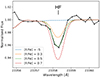 |
Fig. 11. Fitting of the HF line at 23 358 Å in 78 Cnc. The observed spectrum is shown in black, and synthetic spectra with a varying fluorine abundance are shown in different colours. The best-fit abundance for fluorine is 0.5 dex (dashed green line). |
3.2.5. Uncertainties
There are two components to the uncertainties associated with the abundance measurements of chemical species. One component is related to the error associated with the best fit (for abundances derived through spectral synthesis) or with line-by-line scatter (abundances derived through EW). The other component is due to the uncertainties associated with the derived stellar parameters. Therefore, the uncertainties on these parameters need to be propagated into the abundances. To calculate the errors, we employed the method outlined in D’Orazi et al. (2017). Our approach involved evaluating the impact of minor variations (corresponding to 1σ change) in each stellar parameter on the abundance values. We then combined these effects in quadrature to determine the overall uncertainty.
As our sample contains stars that are similar to each other, we constructed the sensitivity matrix for one representative star (HD 218330), which is given in Table 6. For the CNO abundances, we calculated the sensitivity matrix for the optical and IR, but for others, only the optical was calculated. We assumed the errors on CNO abundances in the optical and IR of all the stars in our sample to be the same as calculated for HD 218330, and the errors for the other abundances are given in Tables 5 and 8.
Sensitive matrix with different elements for the optical and IR region of the representative star (HD 218330).
Surface gravity, radius, and mass obtained using scaling relations for red giant stars (Bellinger 2020).
Abundances of yttrium, magnesium, carbon, and nitrogen we used to calculate the ages.
3.3. Asteroseismologic data
As mentioned in the introduction, the sample examined in this paper has been targeted by K2. Reyes et al. (2022) used K2 data and a machine-learning algorithm to extract νmax and Δν for 7 of the 16 stars in our sample. With these two quantities, we determined three sets of stellar parameters, such as mass, radius, and surface gravity, using three different scaling relations. The relations calibrated for solar-type stars, main-sequence stars, and red giant stars were taken from Kjeldsen & Bedding (1995), Bellinger (2019), and Bellinger (2020), respectively. For the Sun, we assumed Teff, ⊙ = 5772 K (Prša et al. 2016), νmax, ⊙ = 3090 μHz, and Δν⊙ = 135.1 μHz (Huber et al. 2011). Tables G.1 and 7 provide the asteroseismic parameters for different relations, and the top panel of Fig. 12 shows the comparison between the spectroscopic and asteroseismic surface gravities. The spectroscopic and asteroseismic values agree well, with a mean difference of 0.18 dex. The difference becomes larger with increasing gravity, however. The trend remains in all three scaling relations because the values are similar to each other. A quick test with the asteroseismic log(g) in MOOG showed that the ionic equilibrium worsens, but remains with 1σ. The effective temperature varies by 25–50 K and microturbulance does not change.
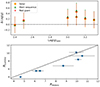 |
Fig. 12. Top: comparison of the surface gravity obtained from spectroscopy and different asteroseimic scaling relations. The yellow circles represent log(g) from the solar-type scaling relation (Kjeldsen & Bedding 1995), the green triangle shows the relation from the main-sequence scaling relation (Bellinger 2019), and the red star shows the relation from the red giant scaling relation (Bellinger 2020). Bottom: comparison of stellar radii obtained from asteroseismology and from the luminosity relation. The dashed black line represents y = x. |
The bottom panel of Fig. 12 shows the comparison between the stellar radii obtained from asteroseismology and from luminosity relation. The radii from the luminosity relation were calculated using the apparent magnitudes in G band and their parallaxes, taken from Gaia. To determine the bolometric magnitude of the stars, we used a Python function14 developed by Creevey et al. (2023) to obtain the bolometric correction. This correction is used to calculate the bolometric magnitude and the luminosity of the star, which later resulted in a measurement of the stellar radius. The two radii have a mean difference of 0.8 ± 0.1 R⊙.
The scaling relations in Bellinger (2020) also provide an estimate for the stellar ages. The relations are reported in Table 7. Along with this, we also derived ages by comparing stellar parameters with stellar evolutionary tracks. Based on the mass and metallicity of a star, we obtained the corresponding stellar evolutionary track from MESA Isochrones & Stellar Tracks (MIST)15 (Dotter 2016). We then compared the Teff and log(g) with the theoretical track to obtain the age. The uncertainties were calculated by randomly drawing 10 000 values of Teff, log(g), mass, and metallicity from four different Gaussian distributions (which were predefined using the spectroscopic and asteroseismic parameters) and comparing them with a grid of MIST evolutionary tracks. Even after this, we were able to improve the uncertainties marginally. The ages obtained from the tracks are consistent with those obtained from the scaling relation.
We further used PARAM (da Silva et al. 2006), a Bayesian estimator, to confirm the asteroseismic ages, masses, and radii. As input, we provided the spectroscopic values for the effective temperature, surface gravity, and metallicity along with νmax and Δν taken from Reyes et al. (2022). PARAM performs a comparison between the input observables and a grid of stellar evolutionary tracks through a Bayesian analysis and outputs posteriors distributions for different parameters. The results from PARAM were consistent with the asteroseismic values for all seven stars.
4. Discussion
The composition of stellar atmospheres can provide useful information with which the evolutionary status of our targets can be probed.
4.1. Lithium
Lithium, a fragile metal, is highly sensitive to temperature variations. It is destructed at low temperatures, approximately 2.5 million K. This corresponds to the temperature at the base of the convective region in stars similar to the Sun. Consequently, during stellar evolution, as the outer envelope becomes mixed through convection, the destruction of lithium occurs readily, resulting in a diminished lithium abundance in evolved stars. Because the stars in our sample are evolved, we expect to obtain a low lithium abundance, as supported by the values presented in Table 5. A(Li) values below 0.25 dex must be considered as upper limits because of the low intensity of the Li Iλ6708 line, whose EW is an upper limit. Only two stars exhibit sufficiently strong lines that enable a reliable estimation of their lithium abundances (HD 22045 and HD 24680).
The analysis of HD 24680 suggests that it is a unique star with an unusually high abundance of lithium, near the threshold for classification as a lithium-rich giant. The high lithium abundance, along with the high observed nitrogen abundance, particularly in the IR region, encouraged us to perform a detailed investigation of its composition, with the aim of understanding the mechanisms of the formation of these stars. HD24680 is classified as an SB1 binary, as also indicated by the large RV error associated with the Gaia average RV.
Therefore, one plausible scenario to explain the high lithium and nitrogen abundances is mass transfer from an intermediate-mass asymptotic giant branch (AGB) companion that has now evolved into a white dwarf. These stars are known to be able to produce Na, Al, and, in a short period of their life, Li, through the Cameron-Fowler mechanism (Ventura & D’Antona 2008). They also produce s-process elements in amounts and relative proportions dependent on their mass and metallicity (see e.g. Cseh et al. 2018). By examining the abundance patterns of elements such as Na, Al, La, Zr, Y, Eu, and Sr (through synthesis), it is possible to gain further insights.
The analysis reveals an increased abundance in s-process elements (listed in Table B.1) with [Sr/Fe] = 0.25 ± 0.16 dex, [Y/Fe] = 0.30 ± 0.06 dex, [Zr/Fe] = 0.40 ± 0.10 dex, and [La/Fe] = 0.46 ± 0.14 dex. Even though the uncertainty on Sr is high because only one line is available, the increase in the abundances of Y, Zr, and La is significant. Along with this, we also observe an over-abundance of Na compared to Al ([Na/Fe] = 0.56 ± 0.07 dex and [Al/Fe] = 0.05 ± 0.10 dex) and a marginal increase in Eu with [Eu/Fe] = 0.15 ± 0.07 dex. While a detailed analysis of the cause of the observed abundance anomalies in this star is beyond the scope of this paper, we note that the overall pattern supports the idea that the surface composition is the result of mass transfer from an low- to intermediate-mass AGB star (2–3 M⊙) that can produce Na and also s-process elements.
4.2. Carbon, nitrogen, and oxygen
As already introduced in Sect. 3.2.1, the analysis of CNO elements in optical and IR spectra reveals a discrepancy between the abundances obtained from the two ranges. It is important to note in this context that the measurements from molecular bands are usually associated with larger uncertainties. This is due to the scatter in the line-by-line abundance within the molecular band, but also to the fact that the strength of the molecular lines is strongly sensitive to atmospheric parameters. The sensitivity matrix provided in Table 6 shows that the errors associated with carbon are approximately 0.16 and 0.15 dex in the optical and IR spectra, respectively. Similarly, for nitrogen, the uncertainties are found to be 0.18 and 0.16 dex for the optical and IR abundances, respectively. Taking these uncertainties into account, we find that the abundances from the two regions for all three elements are consistent in the majority of the stars (as shown in Fig. D.1).
A few stars show a discrepancy beyond those uncertainties. A total of five stars differ in nitrogen, whereas two and three stars differ in carbon and oxygen, respectively. Two reasons come to mind for the high IR abundance, especially for nitrogen: saturation of molecular bands in the optical, and offsets introduced in the analysis by placing more weight on the optical abundance of oxygen. In the optical, carbon and nitrogen were analysed using the CH and CN molecular bands at 4300 Å and 4100 Å, respectively. These bands are crowded, blended with several atomic features, and are saturated. This makes it difficult to obtain an accurate determination of the abundances. In the IR region, the CO band is generally not saturated and rather clean, which makes the IR measurement of carbon more accurate and reliable than the optical. On the other hand, CN is generally weaker, with some blending. This increases the uncertainties on the IR abundance. As the CNO elements are correlated with each other, a bias in one element is propagated to the other two. The oxygen abundance was adopted by placing more weight on the optical value. Even though it is more reliable than the IR value, it is still based on a very small number of features. This might introduce a bias that is propagated into the abundances of carbon and nitrogen and results in an offset.
Table 4, considering the average abundances of carbon, nitrogen, and oxygen, shows that the carbon abundance of most stars lies between −0.1 and 0.0 dex, the nitrogen abundance lies between 0.3 and 0.5 dex, and the oxygen abundance lies between 0.15 and 0.30 dex. As all the stars in the sample are giants, the carbon abundances are quite close to the expected value of −0.1 dex (Gratton et al. 2000). On the other hand, the nitrogen abundance in most of the stars is significantly higher than the expected value of 0.1 dex (Gratton et al. 2000). Two stars, 78 Cnc and HD 97197, are over-abundandent in both nitrogen and carbon. In Fig. 13 we compare our results with those from Böcek Topcu et al. (2019, 2020), and Afşar et al. (2018) because these studies used the same atomic and molecular features to derive the CNO abundances in stars with similar parameters as our sample. We also plot the abundances from the APOGEE (Jönsson et al. 2020) and SAGA database1617 (Suda et al. 2008) as a density and scatter plot, respectively. Our carbon and oxygen abundances are higher than those in the three studies, but still lie within the scatter of APOGEE, but for nitrogen, all three studies are consistent with our results. All studies have a significantly high abundance value relative to the expected values in RGB stars as well as APOGEE, however. The abundances from SAGA show a large scatter in all three elements, which is expected because SAGA contains abundances taken from several different studies.
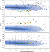 |
Fig. 13. Comparison of the average CNO abundances obtained in this work (red stars) with the literature, such as Böcek Topcu et al. (2019, orange stars), Böcek Topcu et al. (2020, green stars), Afşar et al. (2018, blue stars), the SAGA database (Suda et al. 2008, grey circles), and APOGEE (Jönsson et al. 2020). APOGEE is shown as the density plot in blue. |
These large abundances could be attributed to an offset in the adopted temperatures or to binaries on long-period orbits. If the estimated stellar temperatures were to deviate from the actual value, this might lead to either an over- or an under-estimation of the abundances. For CNO, this effect is amplified because the molecular band is used. For example, when the estimated temperature of a star is higher than the actual value, this results in an increase of carbon abundance because at higher temperatures, it is harder to form molecules such as CH and CN. Therefore, a higher carbon abundance is needed to reproduce the same line strength. Another possibility is that these stars could be part of binary systems with a long-period orbit. The long orbital period makes it hard to identify their binarity. Previous studies have established that the binary fraction of solar-type stars is about 33 ± 2 %, with a period of about 1000 days (Raghavan et al. 2010). The stars might have interacted with their companions in the past, which would result in accretion of large amounts of carbon or nitrogen.
To verify the accuracy of the derived atmospheric parameters and to search for offsets in the estimated stellar temperatures, we made use of the q2 Python package (Ramírez et al. 2014) to determine Teff and log(g) independently, along with a different analysis to estimate the metallicity of the stars. Even though q2 uses the same technique to minimise trends in Fe abundances as is used in MOOG (see Sect. 3.1) to estimate Teff and log(g), it performs the analysis in an automated manner and therefore reduces any biases and errors introduced by the user. By comparison with the spectroscopic parameters that were directly derived using MOOG (shown in Fig. E.1), we found a difference of ΔTeff = 41 ± 23 K, Δlog(g) = 0.13 ± 0.09 dex and Δ[Fe/H] = 0.15 ± 0.08 dex. These differences are not significant given the errors on the spectroscopic parameters. As the q2 and MOOG values are consistent within the errors, we conclude that the stellar parameters obtained from MOOG are a good estimate and do not contain any offsets.
Along with the CNO abundances, we also determined the carbon isotopic ratios (12C/13C) for all the stars. The carbon isotopic ratio is an important quantity to probe the evolutionary phase of a star. This is because a typical solar neighborhood star is expected to form with a C content that mostly consists of 12C with small traces of 13C, leading to a high value of the isotopic 12C/13C ratio. As a star evolves and undergoes the first dredge-up and further mixing processes, the deepening of the convective zone brings 13C to the surface, lowering the isotopic ratio.
In our sample, we find stars with isotopic ratios ranging between 15 and 6. For comparison, the Sun has an isotopic ratio of ∼90 (Ayres et al. 2013), and based on this work, Arcturus has a ratio of 6 ± 3, which is consistent with Abia et al. (2012). Three of the 16 stars (HD24680, HD 77776, and HD 100872) are close to the equilibrium value, that is, the isotopic ratio equals 3. When a star reaches this equilibrium value, the ratio does not decrease any further because the formation rate of 13C is equal to the rate of its destruction. The majority of giant stars have an isotopic ratio of ∼10–15. These isotopic ratios can be explained by additional mixing in the stars, such as thermohaline mixing (Lagarde et al. 2019). According to Lagarde et al. (2019), thermohaline mixing is likely to have a strong effect on the surface abundances of the stars used in this work through their stellar properties. This might also explain the high N abundance and low [C/N] ratio observed in our sample.
4.3. α- and iron-peak elements
In 14 of the 16 stars, we observe a super-solar ratio for the α- and Fe-peak elements. On the other hand, HD 97716 and p04 Leo show sub-solar ratios, especially in elements such as Ca, Ti II, Cr, and Ni. Combined with their metallicity of 0.0 and −0.1 dex, this indicates that they are likely to be thin-disk stars.
Figures 14 and 15 compare the abundances obtained in this work with the abundance from Gaia and APOGEE. For Gaia, we used the Mg and Ca abundances as they are the most reliable from the RVS spectra, and from APOGEE, we obtained CNO, Mg, Si, Ca, Ti I, Ti II, Ni, and Cr. Figure 14 shows an offset of about 0.2 dex in both Mg and Ca with respect to Gaia, whereas APOGEE shows offsets in all the three stars, which can be attributed to the difference in the metallicity reported in our study and in APOGEE.
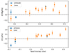 |
Fig. 14. Comparison of the Mg and Ca abundances obtained from this work, Gaia, and APOGEE. The errors are propagations of individual uncertainties. |
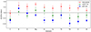 |
Fig. 15. Comparison of the abundances of CNO and the α- and Fe-peak elements obtained from this work and APOGEE. |
4.4. Fluorine
Out of the 16 stars, we obtained reliable fluorine measurements only in 2 stars, that is, HD 22045 and 78 Cnc, with [F/Fe] of 0.35 ± 0.18 and 0.50 ± 0.13 dex, respectively. The two main reasons for the unreliable detections in the other 14 stars are the higher temperatures and the strong telluric contamination. Higher temperatures facilitate dissociating a molecule, due to which, the line strength of the molecules decreases. Ryde et al. (2020) reported a clear signature of destruction of HF molecules in stars with Teff > 4350 K. For stars warmer than 4350 K, they either obtained only upper limits or only measured stars with high fluorine abundance. In our sample, the coolest star has a Teff = 4650 K, and we therefore expect the HF line to be exceedingly weak (which is what we observe). The situation is worsened by the strong telluric contamination in the region around the HF line.
To place the fluorine abundances into context, we compared our results with the literature (Nault & Pilachowski 2013; Li et al. 2013; Jönsson et al. 2017; Guerço et al. 2019; Ryde et al. 2020; Nandakumar et al. 2023), as shown in Fig. 16. We find HD 22045 to be at the upper end of the scatter, whereas 78 Cnc is well above the flat distribution seen for sub-solar metallicity. Abia et al. (2015) suggested that an excess in fluorine abundance ([F/H] > 0.3 dex) was primarily found in stars with C/O close to unity (C/O lower than 1.08). This is followed by 78 Cnc, where the C/O ratio is equal to 0.98.
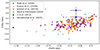 |
Fig. 16. Comparison of the fluorine abundance from this work with the literature. The literature abundances are taken from Nault & Pilachowski (2013, green stars), Li et al. (2013, black circle), Jönsson et al. (2017, orange squares), Guerço et al. (2019, blue crosses), Ryde et al. (2020, brown circles and inverted triangles), and Nandakumar et al. (2023, purple diamonds). Two stars (HD 22045 and 78 Cnc) are shown as blue crosses. |
Even though the two abundances do not allow us to obtain any conclusions on the abundance patterns, these measurements are reported here given the limited number of abundance analyses of fluorine.
4.5. Comparison between ages
The stellar parameters obtained from all three scaling relations are consistent with each other. Even though the asteroseismic ages we obtained are consistent with those from theoretical evolutionary tracks, we found the methods to be equally uncertain in providing a precise measure of the age. The agreement between the two methods showed that the theoretical models are reliable, and we would like to point out that these two methods are not fully independent of each other. The correlation between them arises from the use of the effective temperature and metallicity in the scaling relations and in determination of ages from evolutionary tracks.
We also tested the reliability of the ages obtained from abundance ratios such as [Y/Mg] and [C/N]. The reasoning behind using the first of the two combinations is that magnesium is an α-element, while yttrium is a slow neutron-capture process element. The main process of Mg formation are type II supernovae, that is, massive stars (with mass ≥ 8 M⊙). As massive stars live much shorter lives than low-mass stars, the abundance of Mg is expected to increase quickly. On the other hand, Y is produced through slow neutron capture during the AGB phase of intermediate-mass stars. This process takes a long time as the evolutionary timescale of intermediate-mass star is much longer than that of massive stars. We then expect [Y/Mg] to increase with time, which allows us to probe the stellar ages. Carbon and nitrogen are important ingredients of the CNO cycle. As a star enters the RGB, the increasing depth of the convective zone carries much material from the inner regions into the outer atmosphere. This causes variations in chemical abundances of many elements, specifically, the [C/N] ratio. The dept of the convective zone is directly correlated to the mass of the star and the mass of the star with the age. We can therefore use this ratio to estimate the age. For further details about [Y/Mg] and [C/N] as age estimators, we refer to Berger et al. (2022) and Casali et al. (2019), respectively.
We derived the yttrium abundance through spectral synthesis of 11 lines in the optical region (the line list in Table I.3), as reported in Table 8. The ages were estimated using the relations from Berger et al. (2022) for [Y/Mg] and Casali et al. (2019) for [C/N]. The uncertainties on the ages were determined using a similar method as for the uncertainty on Agetracks, where we randomly drew 10 000 abundance values from a Gaussian distribution, giving a posterior distribution for the age. Table 8 shows that the ages derived from [Y/Mg] are over-estimated when compared to the ages from asteroseismology. For 9 of the 16 stars, [Y/Mg] provides an older age than the Hubble time and is therefore physically impossible (in some cases, even after considering the errors). On the other hand, the ages from [C/N] are under-estimated in comparison with asteroseismology. Most of the stars are reported to be younger than 5 Gyr, with two stars being reported to be older than the Hubble time (with large errors). Because of the disagreement with the asteroseismic ages, which are considered to be quite precise and are backed by the ages from evolutionary tracks, we conclude that the abundance-age relations from Berger et al. (2022) and Casali et al. (2019) are a poor estimate for the stars in our sample.
5. Summary and conclusion
We examined a sample of 16 stars inhabiting the lower RGB and red clump regions. Initially, a spectroscopic analysis was conducted to estimate the stellar parameters, followed by an abundance analysis of various elements such as CNO, α- and Fe-peak elements, Li, Y, and HF. Our focus was on CNO and Li elements to probe the stellar evolutionary phases, while Y was studied because it is one of the elements that are used in chemical clocks. Additionally, we expanded our carbon analysis to include the isotopic ratio, providing further insights into the evolutionary stages of the stars.
All 16 stars were selected from the K2 field as a criterion, allowing us to employ asteroseismology for additional insights. The asteroseismic parameters, including Δ ν and νmax, were obtained from Reyes et al. (2022) for 7 out of the 16 stars. These parameters were then used to estimate stellar masses, radii, surface gravities, and ages using scaling relations. Furthermore, ages were also derived from stellar evolutionary tracks and abundance-age relations based on [C/N] and [Y/Mg].
The derived stellar parameters align well with the values obtained from Gaia and previous literature, except for Hardegree-Ullman et al. (2020). These parameters confirm that these stars lie between the lower RGB and red clump evolutionary phases.
We conducted an analysis in the optical and IR regions to determine the CNO abundances. Our analysis revealed that IR abundances for all three elements were higher than those of their optical counterparts, with N showing the largest disparity. Furthermore, the C and N abundances we obtained for the stars were significantly higher than the expected values for evolved stars (by approximately −0.1 and 0.1 dex, respectively). To rule out the possibility that incorrect stellar parameters might cause these discrepancies, we performed a differential analysis using the q2 tool with three reference stars. The results from q2 were consistent with our analysis. This ensures that our stellar parameters are reliable.
In most cases, the Li line was weak and only allowed us to determine an upper limit on the Li abundance. This is consistent with expectations because lithium is depleted during the ascent of the red giant branch. However, two stars, HD 22045 and HD 24680, exhibited relatively high lithium abundances, with HD 24680 being classified as a Li-rich giant. HD 24680 is classified as an SB1 binary, and therefore, we suspected that it might be a post-mass-transfer object, with an AGB star as the donor (which subsequently evolved into a white dwarf). To investigate this scenario, we analysed elements such as Na, Al, and certain neutron-capture elements (Sr, Y, Zr, La, and Eu). The overabundance of elements such as Na, Sr, Y, and La, along with the absence of an increase in Al, supports the hypothesis of mass transfer from a low- to intermediate-mass AGB star.
The derived mass, radii, and surface gravities using the measurements from Reyes et al. (2022) and three different asteroseismic scaling relations agree well with each other. The ages derived from asteroseismology were confirmed by comparing them with ages obtained from stellar evolutionary tracks.
In recent years, studies such as Berger et al. (2022) and Casali et al. (2019) proposed correlations between elemental abundances and stellar age. To test the reliability of these relations, we compared the ages derived from these correlations with asteroseismic ages. However, the results either over- or under-estimated the ages, depending on the combination of the elemental abundances that were used. Consequently, we conclude that these correlations are not reliable estimators of age within our sample.
In conclusion, we found good agreement between theory and observation, that is, ages from theoretical tracks and asteroseismology. We also identified some peculiarity in the abundances of elements in passing, specifically, nitrogen and Li. We also obtained additional evidence supporting the mass-transfer mechanism for the formation of Li-rich giants. Additional work in terms of constraining the nature of the companion and type of binary interaction, will help to obtain a better understanding, however.
William Herschel Telescope Enhanced Area Velocity Explorer.
4-m Multi-Object Spectroscopic Telescope.
Sloan Digital Sky Survey-Milky Way Mapper.
Apache Point Observatory Galactic Evolution Experiment.
Gaia-European Southern Observatory.
GALactic Archaeology with HERMES.
High Accuracy Radial velocity Planet Searcher for the Northern hemisphere.
We used the standard notations to express the abundances: for an element X, [X] = log ϵ(X)star – log ϵ(X)⊙, [X/Fe] = [X/H] – [Fe/H] and A(ϵ) = log(Nx/NH) + 12.
Large Sky Area Multi-Object Fibre Spectroscopic Telescope.
Data obtained from the INSPECT database, version 1.0 (http://www.inspect-stars.com/).
Stellar Abundances for Galactic Archaeology Database.
Both APOGEE and SAGA data were cleaned to include stars with parameters similar to stars in our sample.
Acknowledgments
We thank Giada Casali and Massimiliano Matteuzzi for useful discussion on asteroseismology. This work presents results from the European Space Agency (ESA) space mission Gaia. Gaia data are being processed by the Gaia Data Processing and Analysis Consortium (DPAC). Funding for the DPAC is provided by national institutions, in particular the institutions participating in the Gaia MultiLateral Agreement (MLA). The Gaia mission website is https://www.cosmos.esa.int/gaia. The Gaia archive website is https://archives.esac.esa.int/gaia. This paper includes data collected by the Kepler mission and obtained from the MAST data archive at the Space Telescope Science Institute (STScI). Funding for the Kepler mission is provided by the NASA Science Mission Directorate. STScI is operated by the Association of Universities for Research in Astronomy, Inc., under NASA contract NAS 5-26555. This research used the facilities of the Italian Center for Astronomical Archive (IA2) operated by INAF at the Astronomical Observatory of Trieste. This work is partially funded by the PRIN INAF 2019 grant ObFu 1.05.01.85.14 (‘Building up the halo: chemo-dynamical tagging in the age of large surveys’, PI. S. Lucatello) and INAF Mini-Grants 2022 (High resolution spectroscopy of open clusters, PI Bragaglia).
References
- Abia, C., Palmerini, S., Busso, M., & Cristallo, S. 2012, A&A, 548, A55 [NASA ADS] [CrossRef] [EDP Sciences] [Google Scholar]
- Abia, C., Cunha, K., Cristallo, S., & de Laverny, P. 2015, A&A, 581, A88 [NASA ADS] [CrossRef] [EDP Sciences] [Google Scholar]
- Abia, C., de Laverny, P., Korotin, S., et al. 2021, A&A, 648, A107 [NASA ADS] [CrossRef] [EDP Sciences] [Google Scholar]
- Afşar, M., Sneden, C., Wood, M. P., et al. 2018, ApJ, 865, 44 [CrossRef] [Google Scholar]
- Ayres, T. R., Lyons, J. R., Ludwig, H. G., Caffau, E., & Wedemeyer-Böhm, S. 2013, ApJ, 765, 46 [NASA ADS] [CrossRef] [Google Scholar]
- Bellinger, E. P. 2019, MNRAS, 486, 4612 [Google Scholar]
- Bellinger, E. P. 2020, MNRAS, 492, L50 [Google Scholar]
- Berger, T. A., van Saders, J. L., Huber, D., et al. 2022, ApJ, 936, 100 [CrossRef] [Google Scholar]
- Blanco-Cuaresma, S., Soubiran, C., Heiter, U., & Jofré, P. 2014, Astrophysics Source Code Library [record ascl:1409.006] [Google Scholar]
- Böcek Topcu, G., Afşar, M., Sneden, C., et al. 2019, MNRAS, 485, 4625 [CrossRef] [Google Scholar]
- Böcek Topcu, G., Afşar, M., Sneden, C., et al. 2020, MNRAS, 491, 544 [CrossRef] [Google Scholar]
- Bressan, A., Marigo, P., Girardi, L., et al. 2012, MNRAS, 427, 127 [NASA ADS] [CrossRef] [Google Scholar]
- Brewer, J. M., Fischer, D. A., Valenti, J. A., & Piskunov, N. 2016, ApJS, 225, 32 [Google Scholar]
- Brown, J. A., Sneden, C., Lambert, D. L., & Dutchover, E. J. 1989, ApJS, 71, 293 [NASA ADS] [CrossRef] [Google Scholar]
- Casali, G., Magrini, L., Tognelli, E., et al. 2019, A&A, 629, A62 [NASA ADS] [CrossRef] [EDP Sciences] [Google Scholar]
- Claudi, R., Benatti, S., Carleo, I., et al. 2017, Eur. Phys. J. Plus, 132, 364 [NASA ADS] [CrossRef] [Google Scholar]
- Cosentino, R., Lovis, C., Pepe, F., et al. 2012, in Ground-based and Airborne Instrumentation for Astronomy IV, eds. I. S. McLean, S. K. Ramsay, & H. Takami, SPIE Conf. Ser., 8446, 84461V [NASA ADS] [Google Scholar]
- Creevey, O. L., Sordo, R., Pailler, F., et al. 2023, A&A, 674, A26 [NASA ADS] [CrossRef] [EDP Sciences] [Google Scholar]
- Cseh, B., Lugaro, M., D’Orazi, V., et al. 2018, A&A, 620, A146 [NASA ADS] [CrossRef] [EDP Sciences] [Google Scholar]
- Cutri, R. M., Skrutskie, M. F., van Dyk, S., et al. 2003, VizieR Online Data Catalog: II/246 [Google Scholar]
- da Silva, L., Girardi, L., Pasquini, L., et al. 2006, A&A, 458, 609 [NASA ADS] [CrossRef] [EDP Sciences] [Google Scholar]
- Deka-Szymankiewicz, B., Niedzielski, A., Adamczyk, M., et al. 2018, A&A, 615, A31 [NASA ADS] [CrossRef] [EDP Sciences] [Google Scholar]
- D’Orazi, V., Gratton, R. G., Angelou, G. C., et al. 2015, MNRAS, 449, 4038 [CrossRef] [Google Scholar]
- D’Orazi, V., Desidera, S., Gratton, R. G., et al. 2017, A&A, 598, A19 [CrossRef] [EDP Sciences] [Google Scholar]
- Dotter, A. 2016, ApJS, 222, 8 [Google Scholar]
- Feuillet, D. K., Bovy, J., Holtzman, J., et al. 2016, ApJ, 817, 40 [NASA ADS] [CrossRef] [Google Scholar]
- Gaia Collaboration 2022, VizieR Online Data Catalog: I/357 [Google Scholar]
- Gaia Collaboration (Brown, A. G. A., et al.) 2021, A&A, 649, A1 [NASA ADS] [CrossRef] [EDP Sciences] [Google Scholar]
- Ghezzi, L., Montet, B. T., & Johnson, J. A. 2018, ApJ, 860, 109 [Google Scholar]
- Gratton, R. G., Sneden, C., Carretta, E., & Bragaglia, A. 2000, A&A, 354, 169 [NASA ADS] [Google Scholar]
- Guerço, R., Cunha, K., Smith, V. V., et al. 2019, ApJ, 885, 139 [CrossRef] [Google Scholar]
- Guerço, R., Ramírez, S., Cunha, K., et al. 2022, ApJ, 929, 24 [CrossRef] [Google Scholar]
- Guggenberger, E., Hekker, S., Basu, S., & Bellinger, E. 2016, MNRAS, 460, 4277 [Google Scholar]
- Gullikson, K., Dodson-Robinson, S., & Kraus, A. 2014, AJ, 148, 53 [NASA ADS] [CrossRef] [Google Scholar]
- Hardegree-Ullman, K. K., Zink, J. K., Christiansen, J. L., et al. 2020, ApJS, 247, 28 [NASA ADS] [CrossRef] [Google Scholar]
- Hekker, S., & Christensen-Dalsgaard, J. 2017, A&ARv., 25, 1 [NASA ADS] [CrossRef] [Google Scholar]
- Hinkle, K., Wallace, L., & Livingston, W. 1995, PASP, 107, 1042 [Google Scholar]
- Hinkle, K., Wallace, L., Valenti, J., & Harmer, D. 2000, Visible and Near Infrared Atlas of the Arcturus Spectrum 3727–9300 A (San Francisco: ASP) [Google Scholar]
- Høg, E., Fabricius, C., Makarov, V. V., et al. 2000, A&A, 355, L27 [Google Scholar]
- Howell, S. B., Sobeck, C., Haas, M., et al. 2014, PASP, 126, 398 [Google Scholar]
- Huber, D., Bedding, T. R., Stello, D., et al. 2011, ApJ, 743, 143 [Google Scholar]
- Jofré, E., Petrucci, R., Saffe, C., et al. 2015, A&A, 574, A50 [Google Scholar]
- Jönsson, H., Ryde, N., Spitoni, E., et al. 2017, ApJ, 835, 50 [CrossRef] [Google Scholar]
- Jönsson, H., Holtzman, J. A., Allende Prieto, C., et al. 2020, AJ, 160, 120 [Google Scholar]
- Kjeldsen, H., & Bedding, T. R. 1995, A&A, 293, 87 [NASA ADS] [Google Scholar]
- Koleva, M., & Vazdekis, A. 2012, A&A, 538, A143 [NASA ADS] [CrossRef] [EDP Sciences] [Google Scholar]
- Kurucz, R. L. 1992, in The Stellar Populations of Galaxies, eds. B. Barbuy, & A. Renzini, 149, 225 [Google Scholar]
- Lagarde, N., Reylé, C., Robin, A. C., et al. 2019, A&A, 621, A24 [NASA ADS] [CrossRef] [EDP Sciences] [Google Scholar]
- Li, H. N., Ludwig, H. G., Caffau, E., Christlieb, N., & Zhao, G. 2013, ApJ, 765, 51 [NASA ADS] [CrossRef] [Google Scholar]
- Lind, K., Asplund, M., & Barklem, P. S. 2009, A&A, 503, 541 [NASA ADS] [CrossRef] [EDP Sciences] [Google Scholar]
- Massarotti, A., Latham, D. W., Stefanik, R. P., & Fogel, J. 2008, AJ, 135, 209 [Google Scholar]
- Mucciarelli, A., & Bellazzini, M. 2020, Res. Notes Am. Astron. Soc., 4, 52 [Google Scholar]
- Nandakumar, G., Ryde, N., & Mace, G. 2023, A&A, 676, A79 [NASA ADS] [CrossRef] [EDP Sciences] [Google Scholar]
- Nault, K. A., & Pilachowski, C. A. 2013, AJ, 146, 153 [NASA ADS] [CrossRef] [Google Scholar]
- Oliva, E., Origlia, L., Maiolino, R., et al. 2012, in Ground-based and Airborne Instrumentation for Astronomy IV, eds. I. S. McLean, S. K. Ramsay, & H. Takami, SPIE Conf. Ser., 8446, 84463T [NASA ADS] [Google Scholar]
- Origlia, L., Oliva, E., Baffa, C., et al. 2014, in Ground-based and Airborne Instrumentation for Astronomy V, eds. S. K. Ramsay, I. S. McLean, & H. Takami, SPIE Conf. Ser., 9147, 91471E [NASA ADS] [Google Scholar]
- Origlia, L., Dalessandro, E., Sanna, N., et al. 2019, A&A, 629, A117 [NASA ADS] [CrossRef] [EDP Sciences] [Google Scholar]
- Placco, V. M., Sneden, C., Roederer, I. U., et al. 2021, Res. Notes Am. Astron. Soc., 5, 92 [Google Scholar]
- Prša, A., Harmanec, P., Torres, G., et al. 2016, AJ, 152, 41 [Google Scholar]
- Raghavan, D., McAlister, H. A., Henry, T. J., et al. 2010, ApJS, 190, 1 [Google Scholar]
- Rainer, M., Harutyunyan, A., Carleo, I., et al. 2018, in Ground-based and Airborne Instrumentation for Astronomy VII, eds. C. J. Evans, L. Simard, & H. Takami, SPIE Conf. Ser., 10702, 1070266 [NASA ADS] [Google Scholar]
- Ramírez, I., & Allende Prieto, C. 2011, ApJ, 743, 135 [Google Scholar]
- Ramírez, I., Meléndez, J., Bean, J., et al. 2014, A&A, 572, A48 [Google Scholar]
- Reyes, C., Stello, D., Hon, M., & Zinn, J. C. 2022, MNRAS, 511, 5578 [NASA ADS] [CrossRef] [Google Scholar]
- Ryde, N., Jönsson, H., Mace, G., et al. 2020, ApJ, 893, 37 [CrossRef] [Google Scholar]
- Sneden, C. 1973, ApJ, 184, 839 [Google Scholar]
- Soderblom, D. R. 2010, ARA&A, 48, 581 [Google Scholar]
- Sousa, S. G., Santos, N. C., Israelian, G., Mayor, M., & Monteiro, M. J. P. F. G. 2007, A&A, 469, 783 [NASA ADS] [CrossRef] [EDP Sciences] [Google Scholar]
- Suda, T., Katsuta, Y., Yamada, S., et al. 2008, PASJ, 60, 1159 [NASA ADS] [Google Scholar]
- Ting, Y.-S., Hawkins, K., & Rix, H.-W. 2018, ApJ, 858, L7 [NASA ADS] [CrossRef] [Google Scholar]
- Ventura, P., & D’Antona, F. 2008, A&A, 479, 805 [NASA ADS] [CrossRef] [EDP Sciences] [Google Scholar]
Appendix A: Comparison of the stellar parameters
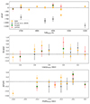 |
Fig. A.1. Comparison of the stellar parameters obtained from this study and Gaia (Creevey et al. 2023), APOGEE (Jönsson et al. 2020), Lamost (Ting et al. 2018), and Hardegree-Ullman et al. (2020). |
Appendix B: Abundances in HD24680
Elemental abundances of elements affected by mass transfer from an AGB star in HD24680.
Appendix C: OH molecular lines in the IR region
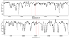 |
Fig. C.1. IR spectrum of HD 4313. The four OH lines we used for analysis are marked with the dashed red line. This shows the problem of weak lines and crowding. |
Appendix D: Comparison of the CNO abundance
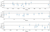 |
Fig. D.1. Comparison of the abundances of CNO elements obtained from the optical and IR spectrum. The y-axis represents the difference between the two abundances. |
Appendix E: Verification of the obtained stellar parameters
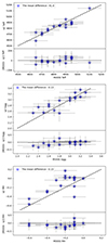 |
Fig. E.1. Comparison of the stellar parameters obtained from q2 and MOOG. |
Appendix F: Fitting of the molecular bands
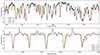 |
Fig. F.1. Fitting of the CH and CO molecular bands in HD218330. The different synthetic lines represent a different carbon abundance. The blue line ([C/Fe] = -5) shows a spectrum with almost no carbon. The carbon abundance of 0.0 dex is the best fit in the CH and CO molecular bands. |
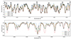 |
Fig. F.2. Fitting of CN in the optical (top panel) and IR (bottom panel) of HD218330. The different synthetic lines represent a different nitrogen abundance. The blue line ([N/Fe] = -5) shows a spectrum with almost no nitrogen. The nitrogen abundances of 0.33 and 0.5 dex are the best-fit in the optical and IR, respectively. |
Appendix G: Asteroseismic parameters for solar and main-sequence scaling relations
Similar to Table 7. The two scaling relations, i.e., solar and main sequence, are taken from Kjeldsen & Bedding (1995) and Bellinger (2019), respectively.
Appendix H: Telluric modelling
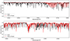 |
Fig. H.1. Telluric modelling of the IR spectra in HD 5214. |
Appendix I: Line list
Line list of the FeI and FeII lines we used to determine the stellar parameters
Line list of the TiI and TiII lines we used to determine the stellar parameters
Line list we used for the abundance analysis of the α- and Fe-peak elements, lithium, and yttrium.
All Tables
Stellar properties (effective temperature, surface gravity, metallicity, and microturbulent velocity) for all the stars in the sample and Arcturus.
Abundances of carbon, nitrogen, and oxygen obtained from the optical and IR region.
Sensitive matrix with different elements for the optical and IR region of the representative star (HD 218330).
Surface gravity, radius, and mass obtained using scaling relations for red giant stars (Bellinger 2020).
Abundances of yttrium, magnesium, carbon, and nitrogen we used to calculate the ages.
Elemental abundances of elements affected by mass transfer from an AGB star in HD24680.
Similar to Table 7. The two scaling relations, i.e., solar and main sequence, are taken from Kjeldsen & Bedding (1995) and Bellinger (2019), respectively.
Line list of the FeI and FeII lines we used to determine the stellar parameters
Line list of the TiI and TiII lines we used to determine the stellar parameters
Line list we used for the abundance analysis of the α- and Fe-peak elements, lithium, and yttrium.
All Figures
|
Fig. 1. Comparison of RV values obtained in this work (indicated by the suffix spec) and Gaia. The errors are the propagated uncertainties on both RVspec and RVGaia. |
| In the text | |
|
Fig. 2. Colour-magnitude diagram of the stars using Gaia magnitudes and parallaxes to compute the absolute magnitude MG. |
| In the text | |
|
Fig. 3. Kiel diagram (Teff vs. log(g)) of the stars using stellar parameters from spectroscopic analysis with an overlay of metallicity. The three dashed lines represent the stellar isochrones with ages of 3 Gyr (blue), 5 Gyr (orange), and 7 Gyr (green), and a metallicity of −0.1 dex. |
| In the text | |
|
Fig. 4. Comparison of the effective temperature obtained from spectroscopy and photometry. |
| In the text | |
|
Fig. 5. Comparison of the stellar parameters (Teff, log(g), and [Fe/H]) with literature sources for Massarotti et al. (2008), Koleva & Vazdekis (2012), Jofré et al. (2015), Feuillet et al. (2016), Brewer et al. (2016), Ghezzi et al. (2018), Deka-Szymankiewicz et al. (2018), Abia et al. (2021). The black line represents the y = 0 line. In all three panels, each colour represents a specific study, as described in the legend. |
| In the text | |
|
Fig. 6. Fitting of two oxygen lines at 6300 and 6363 Å in HD 5214. The observed spectrum is shown as black points, and the synthetic spectra of different oxygen abundances are shown in blue ([O/Fe] = 0.1 dex), orange ([O/Fe] = 0.2 dex), and green ([O/Fe] = 0.3 dex). A line-by-line scatter of 0.1 dex can be seen between the two. |
| In the text | |
|
Fig. 7. Fitting of the OH band at 1.5 and 1.6 μm in HD 218330. The observed spectrum is shown in black, and the synthetic spectra of different oxygen abundances are shown in blue ([O/Fe] = 0.2 dex), orange ([O/Fe] = 0.4 dex), and green ([O/Fe] = 0.6 dex). The vertical dashed black line shows the OH lines considered for the abundance analysis. The best-fit line is shown in orange with O = 0.40 dex. |
| In the text | |
|
Fig. 8. Fitting of 13CO (2–0) band at 23442 Å in HD 6432 to estimate the carbon isotopic ratio. The observed spectrum is shown in black, and the synthetic spectra of varying isotopic ratios are shown in different colours. The best-fit carbon isotopic ratio is 9 (dashed orange line). |
| In the text | |
|
Fig. 9. Comparison of the Li line strength in HD 24680 (black), HD 76445 (red), and HD 99596 (green). The line in HD 24680 is slightly blended with a nearby CN line at 6707.45 Å. |
| In the text | |
|
Fig. 10. Offset and scatter in the line-by-line abundance of α- and Fe-peak elements. The y-axis represents the mean of the standard deviation of the line-by-line abundance (average abundance from all the lines – abundance from the line). The colour represents the scatter of the standard deviation in different stars. The black line represents the offset limit of the mean, beyond which the line is discarded. |
| In the text | |
|
Fig. 11. Fitting of the HF line at 23 358 Å in 78 Cnc. The observed spectrum is shown in black, and synthetic spectra with a varying fluorine abundance are shown in different colours. The best-fit abundance for fluorine is 0.5 dex (dashed green line). |
| In the text | |
|
Fig. 12. Top: comparison of the surface gravity obtained from spectroscopy and different asteroseimic scaling relations. The yellow circles represent log(g) from the solar-type scaling relation (Kjeldsen & Bedding 1995), the green triangle shows the relation from the main-sequence scaling relation (Bellinger 2019), and the red star shows the relation from the red giant scaling relation (Bellinger 2020). Bottom: comparison of stellar radii obtained from asteroseismology and from the luminosity relation. The dashed black line represents y = x. |
| In the text | |
|
Fig. 13. Comparison of the average CNO abundances obtained in this work (red stars) with the literature, such as Böcek Topcu et al. (2019, orange stars), Böcek Topcu et al. (2020, green stars), Afşar et al. (2018, blue stars), the SAGA database (Suda et al. 2008, grey circles), and APOGEE (Jönsson et al. 2020). APOGEE is shown as the density plot in blue. |
| In the text | |
|
Fig. 14. Comparison of the Mg and Ca abundances obtained from this work, Gaia, and APOGEE. The errors are propagations of individual uncertainties. |
| In the text | |
|
Fig. 15. Comparison of the abundances of CNO and the α- and Fe-peak elements obtained from this work and APOGEE. |
| In the text | |
|
Fig. 16. Comparison of the fluorine abundance from this work with the literature. The literature abundances are taken from Nault & Pilachowski (2013, green stars), Li et al. (2013, black circle), Jönsson et al. (2017, orange squares), Guerço et al. (2019, blue crosses), Ryde et al. (2020, brown circles and inverted triangles), and Nandakumar et al. (2023, purple diamonds). Two stars (HD 22045 and 78 Cnc) are shown as blue crosses. |
| In the text | |
|
Fig. A.1. Comparison of the stellar parameters obtained from this study and Gaia (Creevey et al. 2023), APOGEE (Jönsson et al. 2020), Lamost (Ting et al. 2018), and Hardegree-Ullman et al. (2020). |
| In the text | |
|
Fig. C.1. IR spectrum of HD 4313. The four OH lines we used for analysis are marked with the dashed red line. This shows the problem of weak lines and crowding. |
| In the text | |
|
Fig. D.1. Comparison of the abundances of CNO elements obtained from the optical and IR spectrum. The y-axis represents the difference between the two abundances. |
| In the text | |
|
Fig. E.1. Comparison of the stellar parameters obtained from q2 and MOOG. |
| In the text | |
|
Fig. F.1. Fitting of the CH and CO molecular bands in HD218330. The different synthetic lines represent a different carbon abundance. The blue line ([C/Fe] = -5) shows a spectrum with almost no carbon. The carbon abundance of 0.0 dex is the best fit in the CH and CO molecular bands. |
| In the text | |
|
Fig. F.2. Fitting of CN in the optical (top panel) and IR (bottom panel) of HD218330. The different synthetic lines represent a different nitrogen abundance. The blue line ([N/Fe] = -5) shows a spectrum with almost no nitrogen. The nitrogen abundances of 0.33 and 0.5 dex are the best-fit in the optical and IR, respectively. |
| In the text | |
|
Fig. H.1. Telluric modelling of the IR spectra in HD 5214. |
| In the text | |
Current usage metrics show cumulative count of Article Views (full-text article views including HTML views, PDF and ePub downloads, according to the available data) and Abstracts Views on Vision4Press platform.
Data correspond to usage on the plateform after 2015. The current usage metrics is available 48-96 hours after online publication and is updated daily on week days.
Initial download of the metrics may take a while.