| Issue |
A&A
Volume 683, March 2024
Solar Orbiter First Results (Nominal Mission Phase)
|
|
|---|---|---|
| Article Number | A41 | |
| Number of page(s) | 8 | |
| Section | The Sun and the Heliosphere | |
| DOI | https://doi.org/10.1051/0004-6361/202348295 | |
| Published online | 04 March 2024 | |
Efficiency of solar microflares in accelerating electrons when rooted in a sunspot⋆
1
Institute of Physics, University of Graz, 8010 Graz, Austria
e-mail: This email address is being protected from spambots. You need JavaScript enabled to view it.
2
Kanzelhöhe Observatory for Solar and Environmental Research, University of Graz, 9521 Treffen, Austria
3
University of Applied Sciences and Arts Northwestern Switzerland, Bahnhofstrasse 6, 5210 Windisch, Switzerland
4
ETH Zürich, Rämistrasse 101, 8092 Zürich, Switzerland
5
Center for Solar–Terrestrial Research, New Jersey Institute of Technology, Newark, NJ 07102, USA
6
Space Sciences Laboratory, University of California, 7 Gauss Way, 94720 Berkeley, USA
Received:
17
October
2023
Accepted:
27
November
2023
Abstract
Context. The spectral shape of the X-ray emission in solar flares varies with the event size, with small flares generally exhibiting softer spectra than large events, indicative of a relatively lower number of accelerated electrons at higher energies.
Aims. We investigate two microflares of GOES classes A9 and C1 (after background subtraction) observed by STIX onboard Solar Orbiter with exceptionally strong nonthermal emission. We complement the hard X-ray imaging and spectral analysis by STIX with co-temporal observations in the (E)UV and visual range by AIA and HMI to investigate what makes these microflares so efficient in high-energy particle acceleration.
Methods. We made a preselection of events in the STIX flare catalog based on the ratio of the thermal to nonthermal quicklook X-ray emission. The STIX spectrogram science data were used to perform spectral fitting to identify the non-thermal and thermal components. The STIX X-ray images were reconstructed to analyze the spatial distribution of the precipitating electrons and the hard X-ray emission they produce. The EUV images from SDO/AIA and SDO/HMI LOS magnetograms were analyzed to better understand the magnetic environment and the chromospheric and coronal response. For the A9 event, EOVSA microwave observations were available, allowing for image reconstruction in the radio domain.
Results. We performed case studies of two microflares observed by STIX on October 11, 2021 and November 10, 2022, which showed unusually hard microflare X-ray spectra with power-law indices of the electron flux distributions of δ = (2.98 ± 0.25) and δ = (4.08 ± 0.23), during their non-thermal peaks and photon energies up to 76 keV and 50 keV, respectively. For both events under study, we found that one footpoint is located within a sunspot covering areas with mean magnetic flux densities in excess of 1500 G, suggesting that the hard electron spectra are caused by the strong magnetic fields the flare loops are rooted in. Additionally, we revisited a previously published unusually hard RHESSI microflare and found that in this event, there was also one flare kernel located within a sunspot, which corroborates the result from the two hard STIX microflares under study in this work.
Conclusions. The characteristics of the strong photospheric magnetic fields inside the sunspot umbrae and penumbrae where flare loops are rooted play an important role in the generation of exceptionally hard X-ray spectra in these microflares.
Key words: Sun: corona / Sun: flares / Sun: X-rays / gamma rays
Movies associated to Figs. 5 and 9 are available at https://www.aanda.org
© The Authors 2024
 Open Access article, published by EDP Sciences, under the terms of the Creative Commons Attribution License (https://creativecommons.org/licenses/by/4.0), which permits unrestricted use, distribution, and reproduction in any medium, provided the original work is properly cited.
This article is published in open access under the Subscribe to Open model. This email address is being protected from spambots. You need JavaScript enabled to view it. to support open access publication.
1. Introduction
Solar flares are the result of the impulsive release of stored magnetic energy in the solar atmosphere that produces enhanced emission across a wide range of the electromagnetic spectrum. Part of the liberated energy is transferred to accelerated electrons, which can be indirectly observed at hard X-ray wavelengths by bremsstrahlung emission, when energetic electrons interact with the cooler and denser plasma in lower atmospheric layers. As a result, the recorded X-ray spectrum contains information about the energy distribution of non-thermal electrons, which usually are described by a power law (Brown 1971; Lin & Hudson 1976; Holman et al. 2011).
The occurrence rate of flares increases strongly for smaller sizes and energy content, with the flare frequency distribution usually being described by a power law of a slope between 1.5−2.5, derived from different studies of flaring events ranging from nanoflares and microflares to the largest flares observed to date (Dennis 1985; Crosby et al. 1993; Benz & Krucker 2002; Veronig et al. 2002; Christe et al. 2008; Hannah et al. 2011; Purkhart & Veronig 2022). The term microflare commonly describes events that release energies of the order of 1027 erg, about six orders of magnitude less than the largest solar flares (Hannah et al. 2011). It is believed that many processes of larger flares also operate during minor events, but may not be observable as they are masked by the background variations. Other aspects such as the highest energy particles that are typically accelerated in an event may depend on the flare size, with exceptions being observed (Hannah et al. 2008a; Ishikawa et al. 2013; Battaglia et al. 2023).
The non-thermal part of solar flare X-ray spectra (usually observed around above 10 keV) can often be fitted by a power law: I(ϵ)∝ϵ−γ at a photon energy, ϵ, with a photon spectral index, γ (Holman et al. 2011). Statistical studies have reported that smaller events usually show considerably softer X-ray spectra, with a median value of γ = 6.9 (Hannah et al. 2008b) for microflares, compared to a mean value of γ = 3.9 for larger flares observed above 30 keV, as reported by Bromund et al. (1995). For a thick target source region, this photon power law index, γ, is related to the spectral index of the underlying electron flux distribution, δ, via γ = δ − 1 (Brown 1971; Holman et al. 2011). As the number of small events is much larger than that of big flares, some outliers of small flares with hard spectra have previously been observed in the RHESSI flare dataset. Ishikawa et al. (2013) studied six B-class microflares with joint RHESSI and WAM observations and found photon spectral indices γ of the nonthermal spectra between 3.3 and 4.5 and electron energies up to at least 100 keV. So far, the microflare with the hardest HXR spectrum reported is the exceptional GOES A7 event studied in Hannah et al. (2008a), which showed strong non-thermal emission up to energies of over 50 keV and a hard photon power law index of γ = 2.4.
Microflares have been found to occur exclusively in active regions (Stoiser et al. 2007; Hannah et al. 2011), preferably near magnetic neutral lines (Liu et al. 2004). In general, they do not occur directly within sunspots, but in plages (Li & Wang 1998). For bipolar configurations, loop-like morphologies are observed with two footpoints located at opposite magnetic polarities and a thermal source between them (Liu et al. 2004; Stoiser et al. 2007). Jet-like morphologies are also observed in association with microflares. They often show three HXR footpoints, consistent with the interchange reconnection scenario that is commonly invoked to explain open field lines responsible for the escaping plasma and particles (Krucker et al. 2011). For a recent case study, we refer to Battaglia et al. (2023).
The Spectrometer-Telescope for Imaging X-rays (STIX; Krucker et al. 2020) on board the Solar Orbiter spacecraft has been operating since 2020. Since then, it has observed over 20 000 flares. For this study, we searched this extensive STIX flare catalog for microflares with exceptionally hard spectra with an aim to better understand what makes them so efficient at accelerating electrons to high energies.
2. Data and methods
The Solar Orbiter mission is designed to approach the Sun to within 0.28 AU and to reach heliographic latitudes of up to 30° over the course of the mission’s duration (Müller et al. 2020), enabling observations with increased instrument sensitivities. Furthermore, STIX on board Solar Orbiter provides X-ray imaging and spectroscopy of the Sun from 4−150 keV, with an energy resolution of 1 keV at 6 keV and a temporal resolution of up to 0.1 s (Krucker et al. 2020). STIX uses an indirect imaging concept based on 32 individual detectors subdivided into pixels with each detector being located behind fine grids of varying slit width and orientation, resulting in Moire patterns that encode the spatial distribution of the incoming X-ray emission (Krucker et al. 2020). With its energy sensitivity and imaging capability, it is able to observe the evolution of thermal as well as nonthermal flare emission to study electron acceleration and plasma heating during solar flares.
We used the STIX flare catalog to select events up to GOES class C1. We took the recorded STIX quicklook (QL) counts as a proxy for the flare class by using the empirical relation between the GOES 1−8 Å flux f in W m−2 and the distance corrected STIX peak 4−10 keV QL count rate X′: log10(f) = 0.622 − 7.376 log10(X′) published by Xiao et al. (2023).
While the QL data binned into coarse energy bands is continuously sent down from the spacecraft, the pixel data product required for reconstructing STIX images is only transmitted for selected events, thus reducing the number of flares of interest. For the initial selection, we required the ratio of the (10−15) to (4−10) keV counts of the QL channels to be smaller than 0.6. Figure 1 shows this ratio for microflares during the timespan between March 2021 and April 2023. The red line indicates the 0.6 threshold. This condition was fulfilled by 47 out of 20 000 events in the STIX catalog. Requiring the selected events being observed from Earth as well as the STIX point of view further reduces the number to 21 candidates.
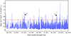 |
Fig. 1. Ratio of STIX QL counts in the (10−15) to the (4−10) keV energy bands during the nonthermal flare peak times for the period March 2021 to April 2023. The red horizontal line indicates the 0.6 threshold. The arrows show the events under study. |
Among the 21 remaining candidates with a QL channel count ratio above 0.6, some are due to counts caused by particle events, others do not have enough counts to perform reliable STIX imaging and one has already been studied (Battaglia et al. 2023). Two of the remaining events stand out in particular: the flares from October 11, 2021 and November 10, 2022 show unusually hard spectra and photons up to high energies during their non-thermal peaks.
During the selected flares, the Solar Orbiter spacecraft was located at distances of 0.69 AU (October 11, 2021) and 0.61 AU (November 10, 2022) from the Sun. The light travel time differences between the spacecraft and Earth are 152.1 s for the event on October 11, 2021 and 187.2 s for November 10, 2022. These shifts are considered in the analysis described below.
The STIX pixel data was used for reconstructing X-ray images. For the spectral analysis, the spectrogram data product was used since it offers the highest time resolution available. The spectrogram data was further binned in time to increase the count statistics for performing spectral analysis with varying integration times. The spectral fitting was done with the OSPEX tool (Schwartz et al. 2002) available in SSWIDL. The functional fits were done with a combination of an isothermal component and a thick target model. For the STIX image reconstruction, the data was integrated over the entire flare duration. For thermal STIX images, the energy range was chosen to be 4−8 keV, while the range 16−28 keV was chosen to contain solely nonthermal counts, as supported by the spectroscopic analysis. For X-ray imaging and spectral fitting, the preflare background was subtracted using the STIX preflare background files closest in time.
For analysis of the flare morphology, EUV observations from the Atmospheric Imaging Assembly (AIA; Lemen et al. 2012) on the Solar Dynamics Observatory (SDO) were used. The AIA data were processed with the standard SolarSoftware (SSWIDL) routines to level 1.5. Helioseismic and Magnetic Imager (HMI; Scherrer et al. 2012) LOS magnetograms were used to determine the magnetic flux density in the flaring region and to get insight into the magnetic field configuration for both events under study. The STIX images were re–projected to the SDO perspective for the comparison with AIA using standard SunPy routines (SunPy Community 2020).
The October 2021 event was also aptly observed by the Expanded Owens Valley Solar Array (EOVSA; Gary et al. 2018), which provides microwave light curves at a 1 s time resolution, spectra at better than a 40 MHz frequency resolution, and images at up to 50 frequency bands in the range between 1−18 GHz. Two of EOVSA’s 13 antennas were not in service on this date, so images were obtained from the 11 remaining antennas. Additionally, the event occurred during a time when the Sun was behind the belt of geosynchronous satellites, which cause radio frequency interference affecting frequencies in the C (3.5−4.2 GHz) and Ku (11.5−12.5 GHz) bands. The microwave burst from this A9 flare reached a surprisingly high radio flux density of 81 sfu (solar flux units; 1 sfu = 1022 W m−2 Hz−1) at its peak frequency of around 5 GHz and showed a prominent quasi-periodic pulsation with a period of 4 s. The data were integrated over the microwave peak time range from 19:23:50–19:23:54 UT to produce images following a self-calibration procedure using the standard CASA (Common Astronomy Software Applications) software. Images at representative frequencies 3.20, 4.82, 5.79, 6.77, 7.74, 8.72, 9.69, 10.67, and 13.27 GHz were compiled, which show a non-thermal spectrum of peak brightness temperatures (66.7, 74.6, 62.5, 45.1, 28.3, 20.8, 15.7, 13.9, and 12.5 MK, respectively) that peaks near 5 GHz.
For our inquiry into the November 17, 2006 flare published by Hannah et al. (2008a), we used white-light data from the Kanzelhöhe Observatory for Solar and Environmental Research (Pötzi et al. 2021) and a Transition Region and Coronal Explorer (TRACE; Handy et al. 1999) 284 Å observation. The TRACE image was processed using the available SSWIDL routines and shifted by x + 3″ and y + 7″ to account for pointing differences, as done in Hannah et al. (2008a). The Kanzelhöhe observation was corrected for differential rotation to match the RHESSI image, since the observation closest in time to the flare was taken around 5 h later. We further created a RHESSI X-ray image using the same detectors and energy range (12−60 keV) as those used in Hannah et al. (2008a).
3. Results
3.1. October 11, 2021
In Fig. 2, we show the STIX, EOVSA, and GOES light curves for the October 11, 2021, microflare under study, with X-ray and radio peak times around 19:24 UT. Following the background subtraction of the preflare interval 18:28–18:42 UT, the flare reaches GOES class A9.
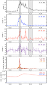 |
Fig. 2. Time evolution of soft and hard X-rays. Light curves of the October 11, 2021 flare. Top four panels: STIX X-ray counts in four selected energy ranges from 4 to 76 keV. Shaded areas indicate timespans considered in the spectral fitting. Second-to-last panel: EOVSA microwave light curves for three selected frequencies. Bottom panel: GOES 1−8 Å (red) and 0.5−4 Å (blue) soft X-ray fluxes. |
Spectral fits to the STIX X-ray spectrum for selected time intervals are shown in Fig. 3. At the first time interval integrated during the impulsive (HXR peak) phase from 19:23:48 UT–19:24:04 UT (left panel), a hard spectrum with δ = (2.98 ± 0.25) is observed. STIX records sufficient counts for reliable spectral analysis up to 76 keV. The thermal plasma is described by a temperature of T = (10.6 ± 1.4) MK and emission measure EM = (36.87 ± 0.04)×1045 cm−3. The spectrum in the right panel during the decay phase is best fitted with a single isothermal component with T = (10.5 ± 0.91) MK and EM = (28.03 ± 0.02)×1045 cm−3.
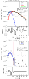 |
Fig. 3. X-ray spectroscopy. Background-subtracted STIX count spectra (black) and best fit (green) from the sum of an isothermal (blue) and a thick target (red) component for October 11, 2021 during the peak (top panel) and decay (bottom panel) phase. Gray vertical lines on the data points indicate the error bars of the count rate. The gray dashed line shows the preflare background spectrum. The red vertical lines show the energy range considered in the fitting. Integration times for the spectral fitting are indicated by gray lines in the top panel of Fig. 2. |
Figure 4 (top row) offers an overview of this event in the 131 Å AIA EUV channel, which is mainly sensitive to plasma around 10 MK during flares (Lemen et al. 2012). In the leftmost panel, three regions that reveal distinct brightening during the flare are observed. The middle panel at 19:24 UT shows loops of hot plasma connecting the flare kernels from the previous panel and an additional loop in the north as well as a jet-like feature in the south. In the right panel, we show that at 19:31 UT (i.e. after the flare energy release has seized), the emission from hot plasma sampled by the 131 Å filter continually decreases. The bottom row of Fig. 4 shows the corresponding evolution in the chromospheric AIA 1600 Å filter with three (left) and four (middle panel) distinct footpoint brightenings being visible corresponding to the brightenings and loops observed in the 131 Å images in the top row. Notably, one of the AIA 1600 Å brightenings is observed inside the sunspot.
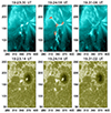 |
Fig. 4. Overview at EUV and UV wavelengths. AIA 131 Å filtergrams over the course of the flare on October 11, 2021 (top) and AIA 1600 Å filtergrams (bottom). Red contours in the top middle panel show footpoint locations derived from the AIA 1600 Å base difference image shown in Fig. 5. Units are given in arcseconds. An animated version of this figure is included online. |
The evolution observed in the AIA 1600 Å filter is further elaborated in Fig. 5, which shows a preflare AIA 1600 Å image from 19:20 UT as a reference in panel a. Panel b reveals four areas of increased brightness during the flare impulsive phase at 19:23:50 UT. The brightening to the far west is located in the umbra of the sunspot. In the base difference image shown in panel d, these enhancements are seen more clearly. Overplotted are contours of STIX spectral images reconstructed in the 4−8 keV (red) and 16−28 keV (green) energy bins. The same contours are also shown on top of an HMI LOS magnetogram in panel c. The non-thermal STIX image recovers two flare kernels visible in the AIA 1600 Å images. The thermal source seen by STIX is located between two flare kernels, namely, the westernmost kernel that is inside the sunspot umbra (located in negative magnetic polarity) and the one just outside the sunspot penumbra to the east (located in positive polarity). The two other kernels are located in negative polarity regions of the trailing plage region.
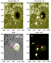 |
Fig. 5. Chromospheric response and magnetograms. AIA 1600 Å images (panels a, b), HMI LOS magnetogram (c) and 1600 Å difference image (d) for October 11, 2021. Green contours show the STIX image in the 16−28 keV energy range, red in 4−8 keV (30, 60, 90% of the maximum intensity). The HMI image is scaled from −700 to +700 G. Units are given in arcseconds. Integration times are 19:23:21–19:24:36 UT for the non-thermal and 19:24:51–19:26:31 UT for the thermal image, respectively. |
The STIX total HXR count fluxes in the 16−28 keV energy range in the footpoints are 0.05 for the umbral kernel and 0.02 [cnts s−1 cm−2 arcsec−2 keV−1] for the eastern kernel. The mean magnetic flux density obtained from the HMI LOS magnetogram in the footpoints observed in 1600 Å is 1544 G, with a standard deviation of ±354 for the western footpoint within the sunspot, (−95 ± 107) G for the northernmost footpoint, (−96 ± 122) G for the north-east and (−37 ± 52) G in the southern location.
Figure 6 shows contours of EOVSA radio images at different frequencies plotted on top of AIA 131 Å and 1600 Å filtergrams. In the left panel, the 20, 50, and 70% contours are shown to illustrate the lower frequency sources extending along the flare loops to the north. In the right panel, only the 50 and 70% levels are shown. This panel clearly shows that the center of the source location gets shifted toward the western flare kernel with increasing frequency, indicative of gyrosynchrotron emission from low in the chromosphere.
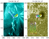 |
Fig. 6. Radio, UV and EUV observations. Contours of EOVSA radio images at various frequencies from 3.20 to 13.27 GHz plotted on top of an AIA 131 Å (left) and 1600 Å (right) filtergram for the event on October 11, 2021. The color code for the different EOVSA frequencies is the same in both images. The contours in the left panel are 20, 50, and 70% of the maximum intensity; in the right panel, we have 50 and 70%. |
3.2. November 10, 2022
Figure 7 shows STIX and GOES light curves for the event of November 10, 2022. The GOES flux after the background subtraction of the preflare interval 17:00–17:11 UT reaches class C1.
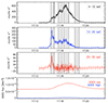 |
Fig. 7. Time evolution of soft and hard X-rays. Light curves of the November 10, 2022 flare. Top panels: STIX counts in selected energy bins from 4 to 50 keV. Bottom: GOES 1−8 Å (red) and 0.5−4 Å (blue) soft X-ray fluxes. Shaded areas indicate the time spans considered in the spectral fitting. |
Functional fits to the X-ray spectrum during the flare are shown in Fig. 8. The top-left panel shows the spectrum during the start of the impulsive flare. The electron distribution power-law index is δ = (4.08 ± 0.23). Initially, the thermal plasma is fitted by a temperature of T = (14.8 ± 6.97) MK and EM = (8.66 ± 0.02)×1045 cm−3. The spectrum steepens to δ = (5.64 ± 0.88) and the EM of the best isothermal fit increases to EM = (43.86 ± 0.04)×1045 cm−3 with a temperature of T = (14.1 ± 2.07) MK for the first thermal peak (top right). For the main thermal peak from 17:16:22−17:17:09 UT (bottom left panel), δ = (5.97 ± 0.26) for the thick target and EM = (80.67 ± 0.04)×1045 cm−3 and T = (13.4 ± 1.02) MK for the isothermal component. During the decay phase shown in the bottom right panel, the best fit is achieved with solely an isothermal component of EM = (187.20 ± 0.04)×1045 cm−3 and T = (9.4 ± 0.27) MK.
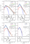 |
Fig. 8. X-ray spectroscopy. Background-subtracted STIX count spectra (black) and best fit (green) from the sum of an isothermal (blue) and a thick target (red) component for November 10, 2022 for four time intervals during the flare evolution (indicated in Fig. 7). Gray vertical lines on the data points indicate the error bars of the count rate. The gray dashed line shows the preflare background spectrum. The red vertical lines show the considered energy range. |
Figure 9 shows the evolution of the flare in the AIA 131 Å filter (see also the accompanying movie). Before the main flare is observed in the STIX and GOES light curves (Fig. 7), a small loop system brightens up in the first frame at 17:12 UT. The main event which coincides with the rise in non-thermal and thermal emission shows a single loop which is clearly enhanced in the second frame at 17:15 UT. This enhancement is accompanied by a southward jet which is still active at 17:17 UT. In the bottom right frame at 17:21 UT the postflare loop is observed.
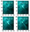 |
Fig. 9. Flare evolution in EUV. AIA 131 Å filtergrams over the course of the flare on November 10, 2022. Units are given in arcseconds. An animated version of this figure is included online. |
The chromospheric response and the photospheric magnetic field are shown in Fig. 10. In the AIA 1600 Å difference image (panel d) between the frames shown in panels a and b, three areas of increased brightness are observed. Contours of these areas are overplotted in blue and purple in panel c. The blue contours show footpoints covering opposite magnetic polarities, with the positive footpoint being located within the sunspot penumbra. The contour shown in purple covers a region of mixed magnetic polarity which indicates the remnant of the separate smaller loop system which brightened up around 17:12 UT.
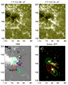 |
Fig. 10. Chromospheric response and magnetograms. AIA 1600 Å images (panels a, b), difference image between them (d) and HMI LOS magnetogram (c) for the November 10, 2022 flare. Green contours show the STIX image in the 16−28 keV energy range, red in 4−8 keV (30, 60, and 90% of the maximum intensity). The HMI image is scaled from −1000 to +1000 G. Blue contours in the HMI image show the areas used for the calculation of the mean magnetic flux densities. The purple contour indicates the area from the AIA 1600 Å base difference image considered to be part of a separate, smaller loop system. Units are given in arcseconds. Integration times are 17:14:05−17:15:25 UT for the nonthermal and 17:15:25−17:17:25 UT for the thermal image respectively. |
Contours of the reconstructed STIX image are overplotted in panels c and d. The non-thermal 16−28 keV image (green) shows two sources which coincide with the chromospheric response to the flare electrons observed in the 1600 Å filter. In the thermal 4−8 keV range (red), a single extended source between the nonthermal footpoints is observed. The STIX contours over the HMI LOS magnetogram in panel c show that the northern HXR footpoint is located within the sunspot penumbra. The mean magnetic LOS flux density within the AIA 1600 Å flare kernels are (1568 ± 350) G for the northern and (−117 ± 137) G for the southern kernel. The STIX summed HXR count fluxes in the 16−28 keV energy range are 0.7 for the umbral kernel and 0.6 [cnts s−1 cm−2 arcsec−2 keV−1] in the southern footpoint outside the sunspot.
4. Discussion
We studied two microflares of GOES classes A9 and C1 with unusually hard X-ray spectra and strong nonthermal emission up to high energies during the impulsive phase observed by STIX. The photon power-law indices, assuming the relation for thick–target bremsstrahlung γ = δ − 1 during the flare impulsive phase, are γ = 1.98 for the October 11, 2021 event and γ = 3.08 in the November 10, 2022 flare. Both events show photons up to high energies considering their small GOES classes, with photon energies up to 76 and 50 keV for the October and November flare, respectively. The spectrum of the previously hardest microflare studied in Hannah et al. (2008a) was best fitted by γ = 2.4 and showed photon energies up to about 50 keV.
For both events in this study, one of the flare footpoints was located directly within a sunspot during the onset, instead of it having moved there over the course of the flare. In the October 11, 2021 A9 flare, one footpoint is located within the sunspot umbra, in strong fields with a mean flux density of (1544 ± 354) G below the AIA 1600 Å kernel. In the flare of November 10, 2022, the northern flare kernel partly covers the sunspot penumbra and umbra with a mean magnetic LOS flux density of (1568 ±350) G. These magnetic flux densities are significantly higher than typical mean values for the mean flux densities in flare ribbons reported by Kazachenko et al. (2017) who did not report values above 1000 G with a 20th–80th percentile range of 408−675 G and the range of 100−800 G reported in Tschernitz et al. (2018) even though they considered flares up to GOES class X17. From extrapolating the relation between flare GOES class and mean magnetic flux density in the flare ribbons of eruptive flares published by Tschernitz et al. (2018) to smaller events, expected values of the flux densities for the A9 and C1 flares in our study are 30 and 67 G, which is one to two orders of magnitude lower than the observed values.
Flares with differences in the magnetic field strength of the flare loop footpoints often show an asymmetry in the HXR fluxes, with the stronger HXR emission being located at the site of weaker magnetic field due to asymmetric magnetic mirroring (Aschwanden et al. 1999; Yang et al. 2012). Despite the significantly stronger magnetic fields in the footpoints located in the sunspots, the STIX flares under study do not show stronger HXR emission from the footpoints located at the weaker magnetic fields outside the sunspot. Possible reasons for such deviations are the electron injection site being located closer to the brighter footpoint (Goff et al. 2004; Falewicz & Siarkowski 2007), varying plasma density along the flare loop (Falewicz & Siarkowski 2007) or differences in the magnetic field convergence along both directions (Yang et al. 2012).
From EOVSA microwave images of the October 11, 2021 event, we find that the locations of the radio sources at typical gyrosynchrotron frequencies shift towards the umbral flare kernel with increasing frequency, in agreement with modeling results of radio emission from an asymmetric loop (Bastian 2000). Microwaves are typically produced by relatively high-energy electrons (∼300 keV). The strong microwave emission seen by EOVSA for the October 2021 A9 event thus indicates that the relatively flat spectrum measured by STIX extends at least to energies of that order. The fact that the EOVSA high-frequency source is located above the sunspot umbra means that the radio-emitting electrons must be able to reach the strong umbral magnetic field region despite a relatively high mirror ratio from this asymmetric loop.
In light of our findings for the two hard STIX microflares, we revisited the hard RHESSI GOES A7 microflare previously reported in Hannah et al. (2008a) using Kanzelhöhe white-light and TRACE EUV data and found that the eastern contours of the nonthermal (12−60 keV) RHESSI image integrated over the impulsive peak are located within the sunspot penumbra and part of the umbra (Fig. 11), analogous to the analyzed STIX events. Umbral flares are rare occurrences as flares usually occur within active regions rather than directly in sunspots, but cases of the former have been reported (e.g., Tang 1978; Joshi & Uddin 1992; Li & Wang 1998). However, these are all studies of regular flares. So far, there have been no studies of umbral microflares carried out to date. In this study, we find that in the two STIX and the one RHESSI microflare with very hard X-ray spectra, at least one footpoint is located directly in a sunspot. We therefore conclude that the characteristics of the strong photospheric magnetic fields inside sunspot umbrae and penumbrae where the flare loops are rooted play an important role in the generation of the exceptionally hard X-ray spectra in these microflares.
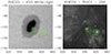 |
Fig. 11. White–light, EUV and X-ray imaging. Kanzelhöhe white-light image from November 17, 2006 and RHESSI 12−60 keV image contours from 05:13:40 to 05:13:52 in green, with 60, 75, and 90% of the maximum intensity (left). TRACE 284 Å EUV filtergram from 05:14:01 UT and same RHESSI contours in green (right). Units are given in arcsec. |
Movies
Movie 1 associated with Fig. 4 Access Supplementary Material
Movie 2 associated with Fig. 9 Access Supplementary Material
Acknowledgments
J.S., A.M.V. and E.C.D. acknowledge the Austrian Science Fund (FWF): I4555-N. A.F.B. is supported by the Swiss National Science Foundation Grant 200021L_189180 for STIX. Solar Orbiter is a space mission of international collaboration between ESA and NASA, operated by ESA. The STIX instrument is an international collaboration between Switzerland, Poland, France, Czech Republic, Germany, Austria, Ireland, and Italy. EOVSA is supported by NSF grant AGS-2130832 to New Jersey Institute of Technology. D.G. acknowledges support from NASA grant 80NSSC18K1128. SDO image data courtesy of NASA/SDO and the AIA science team. HMI data courtesy of NASA/HMI and the HMI science team.
References
- Aschwanden, M. J., Fletcher, L., Sakao, T., Kosugi, T., & Hudson, H. 1999, ApJ, 517, 977 [NASA ADS] [CrossRef] [Google Scholar]
- Bastian, T. 2000, in Encyclopedia of Astronomy and Astrophysics, ed. P. Murdin, 2293 [Google Scholar]
- Battaglia, A. F., Wang, W., Saqri, J., et al. 2023, A&A, 670, A56 (SO Nominal Mission Phase SI) [NASA ADS] [CrossRef] [EDP Sciences] [Google Scholar]
- Benz, A. O., & Krucker, S. 2002, ApJ, 568, 413 [Google Scholar]
- Bromund, K. R., McTiernan, J. M., & Kane, S. R. 1995, ApJ, 455, 733 [NASA ADS] [CrossRef] [Google Scholar]
- Brown, J. C. 1971, Sol. Phys., 18, 489 [Google Scholar]
- Christe, S., Hannah, I. G., Krucker, S., McTiernan, J., & Lin, R. P. 2008, ApJ, 677, 1385 [NASA ADS] [CrossRef] [Google Scholar]
- Crosby, N. B., Aschwanden, M. J., & Dennis, B. R. 1993, Sol. Phys., 143, 275 [NASA ADS] [CrossRef] [Google Scholar]
- Dennis, B. R. 1985, Sol. Phys., 100, 465 [NASA ADS] [CrossRef] [Google Scholar]
- Falewicz, R., & Siarkowski, M. 2007, A&A, 461, 285 [NASA ADS] [CrossRef] [EDP Sciences] [Google Scholar]
- Gary, D. E., Chen, B., Dennis, B. R., et al. 2018, ApJ, 863, 83 [CrossRef] [Google Scholar]
- Goff, C. P., Matthews, S. A., van Driel-Gesztelyi, L., & Harra, L. K. 2004, A&A, 423, 363 [NASA ADS] [CrossRef] [EDP Sciences] [Google Scholar]
- Handy, B. N., Acton, L. W., Kankelborg, C. C., et al. 1999, Sol. Phys., 187, 229 [Google Scholar]
- Hannah, I. G., Krucker, S., Hudson, H. S., Christe, S., & Lin, R. P. 2008a, A&A, 481, L45 [NASA ADS] [CrossRef] [EDP Sciences] [Google Scholar]
- Hannah, I. G., Christe, S., Krucker, S., et al. 2008b, ApJ, 677, 704 [NASA ADS] [CrossRef] [Google Scholar]
- Hannah, I. G., Hudson, H. S., Battaglia, M., et al. 2011, Space Sci. Rev., 159, 263 [NASA ADS] [CrossRef] [Google Scholar]
- Holman, G. D., Aschwanden, M. J., Aurass, H., et al. 2011, Space Sci. Rev., 159, 107 [NASA ADS] [CrossRef] [Google Scholar]
- Ishikawa, S.-N., Krucker, S., Ohno, M., & Lin, R. P. 2013, ApJ, 765, 143 [NASA ADS] [CrossRef] [Google Scholar]
- Joshi, A., & Uddin, W. 1992, Bull. Astron. Soc. India, 20, 75 [NASA ADS] [Google Scholar]
- Kazachenko, M. D., Lynch, B. J., Welsch, B. T., & Sun, X. 2017, ApJ, 845, 49 [NASA ADS] [CrossRef] [Google Scholar]
- Krucker, S., Kontar, E. P., Christe, S., Glesener, L., & Lin, R. P. 2011, ApJ, 742, 82 [Google Scholar]
- Krucker, S., Hurford, G. J., Grimm, O., et al. 2020, A&A, 642, A15 [NASA ADS] [CrossRef] [EDP Sciences] [Google Scholar]
- Lemen, J. R., Title, A. M., Akin, D. J., et al. 2012, Sol. Phys., 275, 17 [Google Scholar]
- Li, W., & Wang, J. 1998, in IAU Colloq. 167: New Perspectives on Solar Prominences, eds. D. F. Webb, B. Schmieder, & D. M. Rust, ASP Conf. Ser., 150, 401 [NASA ADS] [Google Scholar]
- Lin, R. P., & Hudson, H. S. 1976, Sol. Phys., 50, 153 [NASA ADS] [CrossRef] [Google Scholar]
- Liu, C., Qiu, J., Gary, D. E., Krucker, S., & Wang, H. 2004, ApJ, 604, 442 [NASA ADS] [CrossRef] [Google Scholar]
- Müller, D., St. Cyr, O. C., Zouganelis, I., et al. 2020, A&A, 642, A1 [Google Scholar]
- Pötzi, W., Veronig, A., Jarolim, R., et al. 2021, Sol. Phys., 296, 164 [CrossRef] [Google Scholar]
- Purkhart, S., & Veronig, A. M. 2022, A&A, 661, A149 [NASA ADS] [CrossRef] [EDP Sciences] [Google Scholar]
- Scherrer, P. H., Schou, J., Bush, R. I., et al. 2012, Sol. Phys., 275, 207 [Google Scholar]
- Schwartz, R. A., Csillaghy, A., Tolbert, A. K., et al. 2002, Sol. Phys., 210, 165 [NASA ADS] [CrossRef] [Google Scholar]
- Stoiser, S., Veronig, A. M., Aurass, H., & Hanslmeier, A. 2007, Sol. Phys., 246, 339 [NASA ADS] [CrossRef] [Google Scholar]
- SunPy Community (Barnes, W. T., et al.) 2020, ApJ, 890, 68 [Google Scholar]
- Tang, F. 1978, Sol. Phys., 60, 119 [NASA ADS] [CrossRef] [Google Scholar]
- Tschernitz, J., Veronig, A. M., Thalmann, J. K., Hinterreiter, J., & Pötzi, W. 2018, ApJ, 853, 41 [NASA ADS] [CrossRef] [Google Scholar]
- Veronig, A., Temmer, M., Hanslmeier, A., Otruba, W., & Messerotti, M. 2002, A&A, 382, 1070 [NASA ADS] [CrossRef] [EDP Sciences] [Google Scholar]
- Xiao, H., Maloney, S., Krucker, S., et al. 2023, A&A, 673, A142 (SO Nominal Mission Phase SI) [NASA ADS] [CrossRef] [EDP Sciences] [Google Scholar]
- Yang, Y.-H., Cheng, C. Z., Krucker, S., Hsieh, M.-S., & Chen, N.-H. 2012, ApJ, 756, 42 [NASA ADS] [CrossRef] [Google Scholar]
All Figures
|
Fig. 1. Ratio of STIX QL counts in the (10−15) to the (4−10) keV energy bands during the nonthermal flare peak times for the period March 2021 to April 2023. The red horizontal line indicates the 0.6 threshold. The arrows show the events under study. |
| In the text | |
|
Fig. 2. Time evolution of soft and hard X-rays. Light curves of the October 11, 2021 flare. Top four panels: STIX X-ray counts in four selected energy ranges from 4 to 76 keV. Shaded areas indicate timespans considered in the spectral fitting. Second-to-last panel: EOVSA microwave light curves for three selected frequencies. Bottom panel: GOES 1−8 Å (red) and 0.5−4 Å (blue) soft X-ray fluxes. |
| In the text | |
|
Fig. 3. X-ray spectroscopy. Background-subtracted STIX count spectra (black) and best fit (green) from the sum of an isothermal (blue) and a thick target (red) component for October 11, 2021 during the peak (top panel) and decay (bottom panel) phase. Gray vertical lines on the data points indicate the error bars of the count rate. The gray dashed line shows the preflare background spectrum. The red vertical lines show the energy range considered in the fitting. Integration times for the spectral fitting are indicated by gray lines in the top panel of Fig. 2. |
| In the text | |
|
Fig. 4. Overview at EUV and UV wavelengths. AIA 131 Å filtergrams over the course of the flare on October 11, 2021 (top) and AIA 1600 Å filtergrams (bottom). Red contours in the top middle panel show footpoint locations derived from the AIA 1600 Å base difference image shown in Fig. 5. Units are given in arcseconds. An animated version of this figure is included online. |
| In the text | |
|
Fig. 5. Chromospheric response and magnetograms. AIA 1600 Å images (panels a, b), HMI LOS magnetogram (c) and 1600 Å difference image (d) for October 11, 2021. Green contours show the STIX image in the 16−28 keV energy range, red in 4−8 keV (30, 60, 90% of the maximum intensity). The HMI image is scaled from −700 to +700 G. Units are given in arcseconds. Integration times are 19:23:21–19:24:36 UT for the non-thermal and 19:24:51–19:26:31 UT for the thermal image, respectively. |
| In the text | |
|
Fig. 6. Radio, UV and EUV observations. Contours of EOVSA radio images at various frequencies from 3.20 to 13.27 GHz plotted on top of an AIA 131 Å (left) and 1600 Å (right) filtergram for the event on October 11, 2021. The color code for the different EOVSA frequencies is the same in both images. The contours in the left panel are 20, 50, and 70% of the maximum intensity; in the right panel, we have 50 and 70%. |
| In the text | |
|
Fig. 7. Time evolution of soft and hard X-rays. Light curves of the November 10, 2022 flare. Top panels: STIX counts in selected energy bins from 4 to 50 keV. Bottom: GOES 1−8 Å (red) and 0.5−4 Å (blue) soft X-ray fluxes. Shaded areas indicate the time spans considered in the spectral fitting. |
| In the text | |
|
Fig. 8. X-ray spectroscopy. Background-subtracted STIX count spectra (black) and best fit (green) from the sum of an isothermal (blue) and a thick target (red) component for November 10, 2022 for four time intervals during the flare evolution (indicated in Fig. 7). Gray vertical lines on the data points indicate the error bars of the count rate. The gray dashed line shows the preflare background spectrum. The red vertical lines show the considered energy range. |
| In the text | |
|
Fig. 9. Flare evolution in EUV. AIA 131 Å filtergrams over the course of the flare on November 10, 2022. Units are given in arcseconds. An animated version of this figure is included online. |
| In the text | |
|
Fig. 10. Chromospheric response and magnetograms. AIA 1600 Å images (panels a, b), difference image between them (d) and HMI LOS magnetogram (c) for the November 10, 2022 flare. Green contours show the STIX image in the 16−28 keV energy range, red in 4−8 keV (30, 60, and 90% of the maximum intensity). The HMI image is scaled from −1000 to +1000 G. Blue contours in the HMI image show the areas used for the calculation of the mean magnetic flux densities. The purple contour indicates the area from the AIA 1600 Å base difference image considered to be part of a separate, smaller loop system. Units are given in arcseconds. Integration times are 17:14:05−17:15:25 UT for the nonthermal and 17:15:25−17:17:25 UT for the thermal image respectively. |
| In the text | |
|
Fig. 11. White–light, EUV and X-ray imaging. Kanzelhöhe white-light image from November 17, 2006 and RHESSI 12−60 keV image contours from 05:13:40 to 05:13:52 in green, with 60, 75, and 90% of the maximum intensity (left). TRACE 284 Å EUV filtergram from 05:14:01 UT and same RHESSI contours in green (right). Units are given in arcsec. |
| In the text | |
Current usage metrics show cumulative count of Article Views (full-text article views including HTML views, PDF and ePub downloads, according to the available data) and Abstracts Views on Vision4Press platform.
Data correspond to usage on the plateform after 2015. The current usage metrics is available 48-96 hours after online publication and is updated daily on week days.
Initial download of the metrics may take a while.