| Issue |
A&A
Volume 683, March 2024
|
|
|---|---|---|
| Article Number | A184 | |
| Number of page(s) | 9 | |
| Section | Extragalactic astronomy | |
| DOI | https://doi.org/10.1051/0004-6361/202348011 | |
| Published online | 18 March 2024 | |
Galaxy main sequence and properties of low-mass Lyman-α emitters towards reionisation as viewed by VLT/MUSE and JWST/NIRCam
1
Aix-Marseille Université, CNRS, CNES, LAM (Laboratoire d’Astrophysique de Marseille), UMR 7326, 13388 Marseille, France
e-mail: This email address is being protected from spambots. You need JavaScript enabled to view it.
2
Department of Astrophysics, Vietnam National Space Center, VAST, 18 Hoang Quoc Viet, Hanoi, Vietnam
3
Department of Astrophysics, Vietnam National Space Center, Vietnam Academy of Science and Technology, 18 Hoang Quoc Viet, Hanoi, Vietnam
4
Univ. Lyon, Univ. Lyon1, ENS de Lyon, CNRS, Centre de Recherche Astrophysique de Lyon UMR5574, 69230 Saint-Genis-Laval, France
5
Department of Astronomy, Oskar Klein Centre, Stockholm University, AlbaNova University Centre, 106 91 Stockholm, Sweden
6
Max Planck Institute for Astronomy, Köigstuhl 17, 69117 Heidelberg, Germany
7
Institut de Recherche en Astrophysique et Planétologie (IRAP), Université de Toulouse, CNRS, UPS, CNES, 31400 Toulouse, France
8
European Southern Observatory, Karl-Schwarzschild-Str. 2, 85748 Garching, Germany
9
Department of Astronomy, University of Wisconsin-Madison, 475 N. Charter St., Madison, WI 53706, USA
Received:
18
September
2023
Accepted:
22
January
2024
Abstract
Context. Faint, star-forming galaxies are likely to play a dominant role in cosmic reionisation. Great strides have been made in recent years to characterise these populations at high redshifts (z > 3). Now, for the first time, with JWST photometry beyond 1 μm in the rest frame, we can derive accurate stellar masses and position these galaxies on the galaxy main sequence.
Aims. We seek to assess the place of 96 individual Lyman-α emitters (LAEs) selected behind the A2744 lensing cluster with MUSE IFU spectroscopy on the galaxy main sequence. We also compare the derived stellar masses to Lyman-α luminosities and equivalent widths to better quantify the relationship between the Lyman-α emission and the host galaxy.
Methods. These 96 LAEs lie in the redshift range of 2.9 < z < 6.7, with their range of masses extending down to 106 M⊙ (over half with M⋆ < 108 M⊙). We used the JWST/NIRCam and HST photometric catalogues from the UNCOVER project, giving us excellent wavelength coverage from 450 nm to 4.5 μm. We also performed an SED fitting using CIGALE, fixing the redshift of the LAEs to the secure, spectroscopic value. This combination of photometric coverage with spectroscopic redshifts allows us to robustly derive stellar masses for these galaxies.
Results. We found a main sequence relation for these low-mass LAEs of log SFR = (0.88 ± 0.07 − 0.030 ± 0.027 × t) log M⋆ − (6.31 ± 0.41 − 0.08 ± 0.37 × t). This is in relative agreement with the best-fit results of prior collated studies; however, here we see a steeper slope and a higher normalisation. This indicates that low-mass LAEs towards the epoch of reionisation lie above the typical literature main sequence relations derived at lower redshift and higher masses. In addition, by comparing our results to UV-selected samples, we can see that while low-mass LAEs lie above these typical main sequence relations, they are likely not singular in this respect at these particular masses and redshifts. While low-mass galaxies have been shown to play a significant role in cosmic reionisation, our results point to the likelihood that LAEs hold no special position in this regard.
Key words: gravitation / gravitational lensing: strong / galaxies: evolution / galaxies: high-redshift
© The Authors 2024
 Open Access article, published by EDP Sciences, under the terms of the Creative Commons Attribution License (https://creativecommons.org/licenses/by/4.0), which permits unrestricted use, distribution, and reproduction in any medium, provided the original work is properly cited.
This article is published in open access under the Subscribe to Open model. This email address is being protected from spambots. You need JavaScript enabled to view it. to support open access publication.
1. Introduction
The epoch of reionisation is a critical period in the history of the Universe, during which the neutral hydrogen in the intergalactic medium was reionised by the first generations of galaxies, ending around z ∼ 5.5, about one billion years after the Big Bang (McGreer et al. 2015; Bouwens et al. 2015b; Planck Collaboration VI 2020; Bosman et al. 2022). The sources contributing to reionisation are the subject of an ongoing debate in the literature, with a consensus forming around the importance of faint star-forming galaxies (SFGs) (Finkelstein et al. 2015; Livermore et al. 2017; Bouwens et al. 2021; Jiang et al. 2022). However, the importance of massive galaxies Matthee et al. (2022) as well as active galactic nuclei is still discussed (Grazian et al. 2018; Kokorev et al. 2023; Fujimoto et al. 2023).
Among SFGs, the particular importance of Lyman-α emitters (galaxies that display Lyman-α emission at 1215.67 Å rest frame; henceforth, LAEs) has been considered to range from significant (de La Vieuville et al. 2019; Thai et al. 2023) to dominant (Drake et al. 2017). Overall, LAEs tend to be highly star-forming, young, low-metallicity, dust-poor galaxies (Stark et al. 2010, 2011; De Barros et al. 2017; Goovaerts et al. 2023). They have been used extensively as probes of the intergalactic medium (IGM) neutral fraction to examine the progression of reionisation (also see: Stark et al. 2010; Pentericci et al. 2011, 2018; Arrabal Haro et al. 2018; Caruana et al. 2018; de La Vieuville et al. 2020; Kusakabe et al. 2020; Bolan et al. 2022).
Setting further constraints on the properties of these particular galaxies is crucial, considering their likely importance to the process of reionisation (Bouwens et al. 2015a, 2022b). Now, with JWST/NIRCam data pushing wavelength coverage further into the infrared (i.e. to 4.5 μm), extending into the rest-frame optical emission for galaxies between redshifts of 3 and 7, we can obtain more robust estimates for the stellar mass of these high-redshift SFGs.
To access the intrinsically faint regime of galaxies at redshifts between 3 and 7, gravitational lensing by clusters of galaxies is a useful (and often necessary) tool. Using the magnification from lensing, LAEs have been detected at these redshifts with Lyman-α luminosities as low as LLyα ∼ 1039 erg s−1 (Richard et al. 2021; Claeyssens et al. 2022; Thai et al. 2023) and UV-selected sources have been detected down to MUV ∼ −14 (de La Vieuville et al. 2020; Bouwens et al. 2022a; Goovaerts et al. 2023). Using gravitational lensing and the wavelength coverage of NIRCam now allows us to assess the place of intrinsically faint, very-low-mass LAEs on the galaxy main sequence (henceforth, MS) in a robust way.
The MS (at low masses) is a linear and typically tight (∼0.3 dex) relation between the stellar mass and star formation rate of galaxies. Between 108 < M⋆/M⊙ < 1012 and 0 < z < 6, the MS is well understood, even taking into account calibrations between different studies related to the selected initial mass function (IMF), cosmology, selection biases, and SFR indicator (see the reviews of Speagle et al. 2014 (S14) and Popesso et al. 2023 (P23) primarily, as well as Brinchmann et al. 2004; Daddi et al. 2007; Elbaz et al. 2007, 2011; Santini et al. 2009; Sobral et al. 2014; Steinhardt et al. 2014). In S14, a time (or, equivalently, redshift)-dependent form of the MS has been suggested. The authors found that the normalisation and slope of the MS decrease with increasing time (decreasing redshift). This result is also found in the review of P23.
The position of galaxies on the MS gives an indication of what kind of star formation a given galaxy is undergoing. A galaxy residing above the typical MS is a starburst galaxy and a galaxy residing below the typical MS is a quenched galaxy with little to no ongoing star formation.
Previous studies have made it possible to study the low-mass end of the galaxy MS, using lensing, such as Santini et al. (2009, 2017) and at low redshift, such as Boogaard et al. (2018). However, such high-redshift studies have relied on Spitzer/IRAC for their coverage past 1600 Å. More recently, Looser et al. (2023), based on a sample of 200 galaxies observed with JWST/NIRSpec, included estimations of the MS relation down to a very low mass range (∼106 M⊙), in redshift ranges of 2 < z < 5 and 5 < z < 11. They found the galaxies to be located well above the best estimations of the MS at these redshifts and masses. This study, as well as those of Atek et al. (2023) and Maseda et al. (2023), clearly demonstrate the capability of JWST/NIRCam and JWST/NIRSpec to probe these extremely low masses at these redshifts. Atek et al. (2023), in particular, have studied lensed, reionisation-era galaxies, looking to assess the contribution of intrinsically faint, low-mass galaxies to reionisation. These authors managed to derive stellar masses for eight such galaxies, down to log(M⋆/M⊙)∼5.9. Through the study of their ionising properties, they found that these galaxies are likely drivers of the bulk of reionisation.
In this work, we present a first derivation of this MS relation for intrinsically faint, low-mass, lensed LAEs towards the epoch of reionisation (2.9 < z < 6.7). We performed our LAE selection blindly using an integral field unit (IFU): MUSE/VLT. This means our study does not suffer from a biased selection where only the UV-brightest sources would otherwise have been considered. Lensing also helps us to remedy this bias, while also allowing us to access the intrinsically faint and low-mass population dominating cosmic reionisation.
Section 2 presents the spectroscopic and photometric data used. Section 3 covers the details of the SED fitting using secure spectroscopic redshifts from the Lyman-α line. Section 4 presents the results of placing these faint, low-mass LAEs on the galaxy MS, along with a comparison with previous best estimates of the MS relation. This last section also presents conclusions related to the galaxies that have likely played a significant role in cosmic reionisation.
Throughout this paper, the Hubble constant used is H0 = 70 km s−1 Mpc−1 and the cosmology is ΩΛ = 0.7 and Ωm = 0.3. All values of luminosity and UV magnitude are given corrected for magnification and the IMF adopted is that of Salpeter (1955). All equivalent width (EW) values are given in the rest frame.
2. Data: A2744 viewed by MUSE and JWST/NIRCam
We combined MUSE’s IFU spectroscopy of the A2744 galaxy cluster with the full range of imaging available, using the catalogues from the UNCOVER Treasury survey (PIs Labbé and Bezanson, JWST-GO-2561; Bezanson et al. 2022). This photometry is among the deepest available (median catalogue 5σ depth is 29.21 and individual filter depths can be found in Table 1 of Weaver et al. 2024) and ideally suited for the detection and characterisation of high-redshift galaxies.
2.1. MUSE LAEs: LLAMAS
The observations of A2744 form part of the MUSE Lensing Cluster GTO data as well as part of a data release by Richard et al. (2021). The MUSE Lensing Cluster programme contains clusters specifically chosen for efficient amplification of background sources such as high-redshift LAEs. Among these clusters, A2744 has been particularly well studied (e.g. the well known ASTRODEEP and HFF-DEEPSPACE catalogues Lotz et al. 2017; Shipley et al. 2018). A2744 has four MUSE pointings (each 1 × 1 arcmin2) forming a 2 × 2 mosaic with exposures of between 3.5 and 7 hours. Sources are identified in the MUSE datacube using the MUSELET software (Piqueras et al. 2017)1, Marz software (Hinton 2016), and Source Inspector package (Bacon et al. 2023). These packages allow the user to define redshifts for objects based on identification of emission and absorption features, as well as HST images of sources and redshift suggestions from Marz. The spectroscopic catalogue for A2744, originally presented in Mahler et al. (2018) and improved by Richard et al. (2021), is publicly available2.
The LAEs identified behind A2744 form part of the Lensing Lyman Alpha MUSE Arcs Sample (LLAMAS) (Claeyssens et al. 2022). Only LAEs with a high redshift confidence level from the LLAMA sample were used in this work. Magnifications for all sources were noise-weighted means across each pixel in the source, calculated using the lens model from Richard et al. (2021) and the LENSTOOL software (Kneib et al. 1996; Jullo et al. 2007). For A2744, there are 154 images of 121 individual LAEs. It contains the most LAEs of all the LLAMAS clusters, making it ideal for this single cluster study.
The flux for these LAEs was determined using the method detailed in de La Vieuville et al. (2019) and Thai et al. (2023). This method uses SExtractor (Bertin & Arnouts 1996) on the continuum-subtracted narrow band (NB) datacube in which each LAE was detected.
2.2. JWST/NIRCam data
The photometry used for this study comes from the UNCOVER treasury survey (Bezanson et al. 2022). The photometric catalogues themselves are described in Weaver et al. (2024) and Kokorev et al. (2022)3. This survey combines HST data from the F435W, F606W, F814W, F105W, F115W, F125W, F140W, and F160W filters with NIRCam data from the F090W, F150W, F200W, F277W, F356W, F410M, and F444W bands. This wide range offers excellent coverage from 15 bands between 400 nm and 4.5 μm.
Weaver et al. (2024) subtracted the bright cluster galaxies (BCGs) and intra-cluster light (ICL) in order to better detect faint galaxies. The detection is then performed on a combination of the F277W, F356W, and F444W bands, along with the PSF (point spread function) matched to the F444W band. Two photometric catalogues were then created with a 0.32″-aperture catalogue being optimised for faint, compact sources.
Of the 154 images of MUSE LAEs in the MUSE field of view, 121 images were detected in the UNCOVER photometry, of 99 individual LAEs. Due to the extended nature of some lensed LAEs, they were identified as two continuum objects. Therefore, in this case, we combined the fluxes of the continuum objects. This occurred in seven cases. In two cases, we rejected the continuum associated to an LAE as it is clearly coming from a BCG. Ultimately, we chose a representative for each multiple image system with the least contamination possible. We removed one more object as it is extremely highly magnified (magnification factor 135), meaning that the uncertainty on the derived SFR and stellar mass would be too great. Thus, there were 96 individual LAEs remaining in our final sample.
With a magnification factor range of 1.5–9.5 and a sample average magnification of 3, the resultant Lyman-α luminosities we probed are in the range 40 < log10(LLyα/erg s−1) < 43. The UV magnitude range is −23 ≲ MUV ≲ −14, where this value is derived from the filter closest to the 1500 Å rest frame emission, in the same way as Goovaerts et al. (2023). The redshift and absolute magnitude distribution is displayed for the 96 LAEs in Fig. 1, colour-coded by the lensing magnification of each galaxy. We can see from this plot that our sample populates a large part of the MUV space between a current blank field limit for a similar study of LAEs in the literature (Kusakabe et al. 2020) and the typical integration limit applied to the UV luminosity function when calculating the total star formation rate density, which is the operative quantity when considering whether a population can reionise the neutral IGM (Bouwens et al. 2022b).
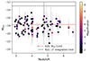 |
Fig. 1. Distribution of the 96 individual LAEs used in this study in redshift and absolute UV magnitude, colour-coded by lensing magnification. Redshifts quoted are spectroscopic from MUSE and magnitude values are derived from the filter that covers the rest frame 1500 Å emission. Horizontal dashed lines denote relevant limits: red denotes the MUV limit in an equivalent blank field study (Kusakabe et al. 2020) and black denotes the integration limit used when calculating the star formation rate density from the UV luminosity function (LF) in the latest study (Bouwens et al. 2022b). |
3. SED fitting with CIGALE
CIGALE, which stands for Code Investigating GALaxy Emission (Boquien et al. 2019), is a Python code4 designed to extract galaxy properties from photometric and spectroscopic observations ranging between the far UV to radio. It takes into account flexible star formation histories (SFHs), nebular emission, and different dust attenuation models. We fit the observed photometry of all the JWST-detected LAE images in A2744 (121 out of 154). We took advantage of the accurately known, secure spectroscopic redshifts available for these LAEs, fixing these values in CIGALE. We also subtracted Lyman-α fluxes from the filters that see them so they do not contaminate the photometry.
We investigated two different SFHs: a single exponentially decaying burst and a double burst model with an initial burst of star formation followed by a second, delayed burst (Małek et al. 2018; Boquien et al. 2019). A range of ages are taken into account in both models, from 10 − 700 Myr. Mass fractions for the delayed burst range from 0.001 to 0.65. The best-fit of these two SFHs is carried forward for analysis.
We use the stellar library of Bruzual & Charlot (2003) with five metallicities ranging between 0.0001 and 0.02. We take into account nebular emission as some high-redshift galaxies can exhibit strong nebular lines (Maseda et al. 2020; Schaerer et al. 2022; Matthee et al. 2023; Brinchmann 2023). The nebular models used by CIGALE (Theulé et al., in prep.) are computed using the CLOUDY software Ferland et al. (2017). Gas metallicities used range between 0.0004 and 0.02. Dust attenuation in our galaxies is modelled based on the modified starburst attenuation curve from Calzetti et al. (2000).
CIGALE outputs the required physical parameters of each galaxy, in this case stellar mass, SFR, and the  statistic for each fit. To check the consistency of these results and the reliability of the CIGALE fitting, we use CIGALE’s mock_flag function to generate mock results with simulated noise, to which we compare the actual results in order to assess how reliably we estimate parameters such as the mass and SFR. This comparison is detailed in Appendix A.
4. Results
4.1. Lyman-α luminosity to stellar mass relation
Following the analyses of Santos et al. (2020, 2021) we can assess the relationship between stellar mass and both Lyman-α luminosity and Lyman-α equivalent width (EWLyα). This can help to evaluate the connection between the host galaxy and its Lyman-α emission. Due to the complicated nature of Lyman-α transfer and escape (Verhamme et al. 2008; Leclercq et al. 2017; Matthee et al. 2021; Blaizot et al. 2023), this connection is still under much discussion. These relationships between stellar mass and Lyman-α parameters are shown in Fig. 2.
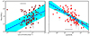 |
Fig. 2. Stellar mass vs Lyman-α parameters. Left: stellar mass plotted against Lyman-α luminosity. Right: stellar mass plotted against EWLyα. Blue dashed lines indicate linear fits to the data and cyan shaded areas the 1σ uncertainties on the fits, details of which are given in the text. Median uncertainties on the Lyman-α parameters are shown by the horizontal black error bars. |
Fitting a linear relationship between Lyman-α luminosity and stellar mass for our 96 LAEs, we find log(M⋆/M⊙) = (0.85 ± 0.17) log(LLyα/erg s−1) − (27.8 ± 6.4). This result has a large dispersion but is in rough agreement with that in Santos et al. (2021) (albeit with a lower slope and normalisation), which is especially interesting as the 4000 SC4K LAEs in that study are in a Lyman-α luminosity range of 4.25 ≲ log(LLyα)(erg s−1) ≲ 44; therefore, they are far brighter than our sample. Our results suggest that this relationship holds down to intrinsically faint LAEs: when a galaxy displays Lyman-α emission, the connection between the stellar mass of the galaxies and the amount of Lyman-α luminosity they emit remains roughly constant across all currently-accessible luminosities. However, there is significant scatter in the data, which is to be expected, and indicative of the wide variety of conditions within galaxies affecting Lyman-α escape. If a given galaxy lies far above this best-fit relation (blue dashed line in Fig. 2), it is emitting far less Lyman-α emission than expected for a galaxy of its mass. This likely indicates other factors at play, such as higher dust content or specific viewing angles (Atek et al. 2008; Verhamme et al. 2008; Chen et al. 2024). Given the dispersion in the left panel of Fig. 2, these are clearly important effects. For example, the object at 1040 erg s−1 lies ∼3σ away from the best fit relation, indicating that some property of this galaxy prevents the escape of Lyman-α photons more than usual for LAEs at this redshift and mass range. Estimating the dust content and extinction from data taken at longer wavelengths could help to shed more light on this issue.
When comparing EWLyα with the stellar mass, we find a linear relationship that takes the following form: log(M⋆/M⊙) = ( − 0.62 ± 0.07) log(EWLyα)+(9.1 ± 0.1). This is a tighter relationship than is seen for the luminosity, which is unsurprising as the UV magnitude used to calculate EWLyα is tightly correlated with the stellar mass (Duncan et al. 2014; Santini et al. 2023). This suggests that Lyman-α photons end up having a relatively harder time escaping higher mass galaxies. This is likely due to the higher dust content in galaxies of higher masses (Zahid et al. 2013; Calura et al. 2017; Donevski et al. 2020). While this relation is tighter than that between stellar mass and luminosity, a dispersion is still evident around the best-fit relation. This indicates that for a given mass, a range of Lyman-α escape scenarios are possible. A more complete study on these relations requires larger samples of lensed galaxies which can be binned in terms of stellar mass. We return to this in Sect. 5.
4.2. Star formation main sequence
We plotted the best-fit stellar masses and SFRs derived from CIGALE in Fig. 3. This was done for the first time for lensed LAEs of these masses at these redshifts. Therefore, in order to gain an understanding of how these galaxies compare to galaxies of higher mass and UV-selected samples, we incorporated the appropriate best fits from the reviews of S14 and P23, as well as data from S17, a similar study to ours (without the benefit of JWST data) using Lyman break-selected galaxies (LBGs) in the Hubble Frontier Fields (HFF). Additionally, we compared the 96 LAEs to the sample of LBGs selected behind A2744 from Goovaerts et al. (2023) (specifically, the LBG-only galaxies, which show no Lyman-α emission). For the LBGs, an identical fitting process was used to the LAEs, as detailed in the previous section. We chose to adopt the time-dependent form of S14 to fit to our data. As we have not probed the higher mass end of the MS, where its linearity breaks down (see P23 and references therein), this linear form for the MS is safe for us to adopt. This form of the MS is given as:
 (1)
(1)
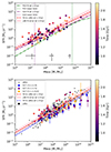 |
Fig. 3. Stellar mass vs SFR: the galaxy MS. Upper panel: 96 LAEs in our final sample plotted on the star-forming MS, together with the best fits to the data of P23, S14 and the best fit to the LAEs following Eq. (1). LAEs are colour-coded by as ‘Time’, in Gyr, which is the age of the Universe at the observed redshift. The purple, dotted line indicates the lowest-stellar mass limit of S14’s review (2 × 10⁷ M⊙) and the green, dotted line indicates the lowest-stellar mass limit of P23’s review (6 × 10⁹ M⊙). The pink shaded area denotes the ±1σ area for the best-fit MS relation at the sample mean age, ∼1.48 Gyr. The mean error bars in three mass bins (106 < M/M⊙ < 2.5 × 10⁷, 2.5 × 10⁷ < M⋆/M⊙ < 5 × 10⁸ and 5 × 10⁸ < M⋆/M⊙ < 1010) are shown in black at the bottom of the plot. Lower: same LAEs and best-fit relation, but compared this time to the results in the same mass range that have been UV-selected, namely: the LBGs from A2744 from Goovaerts et al. (2023) as grey diamonds, with a blue best-fit relation, and the mass-binned results from S17 as coloured diamonds with error bars. |
The values of the constants a, b, c, and d are given in Table 1, both for this work and for those we compare to. We adjusted the relations quoted in S14 and P23 to take into account the different IMFs used. We used the Salpeter IMF (Salpeter 1955) in our SED fitting, but the Kroupa IMF (Kroupa 2001) was used in both of the reviews we used as the basis of our comparison. This necessitates a correction to the stellar masses, which we carried out following the prescription in both S14 and P23 (taken from Zahid et al. 2012) to M⋆, K = 0.62M⋆, S where M⋆, K and M⋆, K are the stellar masses calculated using a Kroupa IMF and a Salpeter IMF, respectively. These corrections are incorporated in the dashed lines in Fig. 3, but the original quoted fit values are given in Table 1.
Results for the galaxy MS from the literature and from this study.
It is evident from the upper panel of Fig. 3 that the low-mass LAEs studied here lie above the fits to the MS calibrated at higher masses. Thus, a question arises as to why these low-mass LAEs lie above these MS relations, and whether this a result of the selection of these galaxies as LAEs or whether this is rather a result of their low mass. We have sought to answer this through comparison to the aforementioned datasets. The most stark difference is seen when making a comparison to the fit of P23. The authors of this review fit their data to a relation of the form:
 (2)
(2)
with a0 = 2.693 ± 0.012, a1 = −0.186 ± 0.009, a2 = 10.85 ± 0.05, a3 = −0.0729 ± 0.0024, and a4 = 0.99 ± 0.01. This fit is designed to take into account the turnover of the MS at high masses (M⋆ > 1010); however, it performs poorly when compared to our sample, especially in the low-mass regime. We see a 0.43 dex difference at 107 M⊙ and a 0.19 dex difference at 1010 M⊙. This difficulty in fitting the low-mass LAEs is unsurprising as the P23 relation was derived using galaxies down to a lower mass limit of 108.5 M⊙.
The fit from S14, which takes the form displayed in Eq. (1), fits the data better (noting the error of ∼0.3 dex in their MS relation). We see a 0.13 dex difference at 107 M⊙ and a 0.17 dex difference at 1010 M⊙, with S14’s relation having been derived using galaxies of mass down to 107.3 M⊙. However only two studies with galaxies of mass below 108 M⊙ were included, and S14 did not incorporate the first two Gyr of galaxy evolution in their fit, limiting its usefulness as a comparative tool to this study. Nevertheless, this best-fit relation is consistent with ours within the respective errors.
The fit of the expression in Eq. (1) that we have found for our LAEs is log SFR = (0.88 ± 0.07 − 0.030 ± 0.027 × t) log M⋆ − (6.31 ± 0.41 − 0.08 ± 0.37 × t). The ±1σ error region is shaded in pink on both plots in Fig. 3. We stress that given the conclusions above, this relation and uncertainty likely do not hold for the lower (and higher) mass regions of this graph, which our data do not probe. The constants of our best fit that are not time-dependent (a and c in Eq. (1)) are consistent within their uncertainties with the best fit of S14, and we see a similar but less significant evolution with time (constants b and d in Eq. (1)). This points to galaxies selected as LAEs across our redshift range as being consistently young and with a high rate of star formation. However, a less significant evolution may also be due in part to our sample being smaller than that of S14. Details of the fitting for the LAEs and LBGs in this work, as well as comparisons to S14 and Santini et al. (2017, henceforth, S17), are given in Table 1.
The discrepancy between our results and the collations of S14 and P23, as mentioned, likely comes from the difference in mass-range probed, but to further verify this, we made a comparison with two UV selected samples in the lower plot of Fig. 3: S17, conducted on the HFF galaxy clusters and the selection of LBGs from Goovaerts et al. (2023), (294 galaxies), selected behind A2744 itself, in the same volume as the LAEs in this work. The fit to the LBGs (blue dashed line) is (0.89 ± 0.11 − 0.024 ± 0.007 × t) log M⋆ − (6.75 ± 0.78 − 0.09 ± 0.59 × t). This relation is consistent with that for the LAEs, further suggesting that it is the mass (and redshift) range probed, rather than the selection of the sample by Lyman-α emission that differentiates these galaxies from MS relations in the literature. A small effect can be seen in the lower panel of Fig. 3; the LAE and LBG best fits show a better agreement in the higher mass range than the lower mass range, but this effect is at a low level of confidence (< 1σ) for this dataset.
The mass-binned data of S17 are in good agreement with our data, particularly in the highest redshift bin (5 < z < 6.6). They also found a similar trend when considering earlier times (higher redshifts), namely: an increasing normalisation, but a similar slope compared to later times (lower redshifts). However this evolution is more dramatic in their data than ours. This could be due to their larger sample size; however uncertainties related to the lack of wavelength coverage past 400 nm above z = 3 may have an effect. This photometry can be especially problematic in crowded fields such as lensing clusters (Laporte et al. 2015; Goovaerts et al. 2023). The 2σ-clipping procedure used in S17 and the choice to calculate the MS according to log SFR = α log (M/M9.7)+β (where M9.7 = 109.7 M⊙) may also play a role.
The role of stellar mass is additionally supported by very recent results from Nakane et al. (2023), who found that high-redshift (z > 7) LAEs (and LBGs) in a higher mass range than those covered in this study (most galaxies exhibit M⋆/M⊙ > 108) typically lie on the MS (the reference MS in this case is from S17); however, these results (similarly to our own) see a lot of scatter in individual data points. Additionally supporting the conclusions of this work, the authors made no significant distinction between the LAE and non-LAE populations in terms of their position on the MS.
Viewed together, these results indicate that, while the low-mass LAEs in this study reside above the typical MS estimates derived from higher mass samples, particularly that of P23 (derived for galaxies of much higher mass), they are likely similar to galaxies that are not LAEs, but are of similar mass at similar redshifts. This points to an enhanced specific SFR in these low-mass populations, but no special role for LAEs themselves. In the context of cosmic reionisation, this supports the conclusion that while low-mass galaxies play an important role, LAEs are likely not singular in their impact on this process.
5. Conclusions
With new JWST/NIRCam data, secure spectroscopic redshifts from VLT/MUSE and CIGALE SED fitting, we have obtained reliable estimates for the SFR and stellar mass for intrinsically faint, lensed, reionisation-era LAEs. This allowed us to place these galaxies on the star-forming main sequence and compare them to UV-selected samples as well as studies conducted at higher mass. We also compared stellar masses for these galaxies with Lyman-α observables. Our conclusions are summarised as follows:
– The relation we find for stellar mass and Lyman-α luminosity: log(M⋆/M⊙) = (0.85 ± 0.17) log(LLyα/erg s−1) − (27.8 ± 6.4), agrees with similar relations found for samples of LAEs with higher masses. This indicates that the general relation between stellar mass and the amount of Lyman-α emission observed from a galaxy holds well over the range of currently observed LAEs.
– We note that this relation has a large dispersion, which reflects the scatter of the data. This indicates that there is a range of Lyman-α escape scenarios for galaxies of the same mass. This likely depends on the dust extinction of the galaxies, as well as on the viewing angle and geometry, but longer-wavelength observations that quantify dust content and extinction are necessary to confirm this.
– The relation between Lyman-α EW and stellar mass is tighter than for Lyman-α luminosity: log(M⋆/M⊙) = ( − 0.62 ± 0.07) log(EWLyα)+(9.1 ± 0.1). This anticorrelation suggests that Lyman-α photons find it harder to escape higher mass galaxies.
– The MS relation we find for our LAEs between redshifts of 2.9 and 6.7, and masses of 106 M⊙ and 1010 M⊙ is log SFR = (0.88 ± 0.07 − 0.030 ± 0.027 × t) log M⋆ − (6.31 ± 0.41 − 0.08 ± 0.37 × t). This relation is consistent with the best-fit found in S14, which is derived using galaxies down to 107.3 M⊙, and agrees well with galaxies not selected as LAEs at similar masses and redshifts. However a clear discrepancy is seen between this relation and the best-fit of P23 which is derived only using galaxies of stellar masses greater than 108.5 M⊙.
– Our results suggest that the mass range probed is the main influence in our determination of the galaxy main sequence relation, more than the selection of our sample by their Lyman-α emission. In the context of cosmic reionisation, although low-mass galaxies have been shown to play a significant role, our results also suggest that LAEs do not distinguish themselves in this process as they have no particular enhanced sSFR, compared to the general population of star-forming galaxies at this time.
Larger samples of this type, which are necessary for obtaining more precise estimations of the main sequence relation for both LAEs and UV-selected samples, will have to wait until further imaging of lensing clusters with JWST/NIRCam. Observing many lensing clusters with the required depth of photometry is expensive and A2744 has been prioritised thus far. However in the coming months and years, we can expect samples of this type to grow significantly, with the addition of further lensing clusters containing hundreds of LAEs in and around the epoch of reionisation. Samples with JWST/NIRSpec data are doubly valuable, as they enable SFR determinations using Hα luminosities for these redshifts, as well as full spectral fittings for more accurate galaxy properties. Large samples with accurate Hα luminosity determinations are hard to obtain and they have not been a priority for the redshifts considered in this work. Future JWST Cycles larger samples with better data are likely to become available, thus allowing for more comprehensive studies.
Acknowledgments
The authors would like to thank the anonymous referee for numerous useful comments which helped in improving this article. This work is done based on observations made with ESO Telescopes at the La Silla Paranal Observatory under programme IDs 060.A-9345, 092.A-0472, 094.A-0115, 095.A-0181, 096.A-0710, 097.A0269, 100.A-0249, and 294.A-5032. Also based on observations obtained with the NASA/ESA Hubble Space Telescope, retrieved from the Mikulski Archive for Space Telescopes (MAST) at the Space Telescope Science Institute (STScI). STScI is operated by the Association of Universities for Research in Astronomy, Inc. under NASA contract NAS 5-26555. All plots in this paper were created using Matplotlib (Hunter 2007). Part of this work was supported by the French CNRS, the Aix-Marseille University, the French Programme National de Cosmologie et Galaxies (PNCG) of CNRS/INSU with INP and IN2P3, co-funded by CEA and CNES. This work also received support from the French government under the France 2030 investment plan, as part of the Excellence Initiative of Aix-Marseille University – A*MIDEX (AMX-19-IET-008 – IPhU). Financial support from the World Laboratory, the Odon Vallet Foundation and VNSC is gratefully acknowledged. Tran Thi Thai was funded by Vingroup JSC and supported by the Master, PhD Scholarship Programme of Vingroup Innovation Foundation (VINIF), Institute of Big Data, code VINIF.2023.TS.108. Pham Tuan-Anh was funded by Vingroup Innovation Foundation (VINIF) under project code VINIF.2023.DA.057.
References
- Arrabal Haro, P., Rodríguez Espinosa, J., Muñoz-Tuñón, C., et al. 2018, MNRAS, 478, 3740 [NASA ADS] [CrossRef] [Google Scholar]
- Atek, H., Kunth, D., Hayes, M., Östlin, G., & Mas-Hesse, J. M. 2008, A&A, 488, 491 [NASA ADS] [CrossRef] [EDP Sciences] [Google Scholar]
- Atek, H., Labbé, I., Furtak, L. J., et al. 2023, arXiv e-prints [arXiv:2308.08540v1] [Google Scholar]
- Bacon, R., Brinchmann, J., Conseil, S., et al. 2023, A\&A, 670, A4 [Google Scholar]
- Bertin, E., & Arnouts, S. 1996, A&AS, 117, 393 [NASA ADS] [CrossRef] [EDP Sciences] [Google Scholar]
- Bezanson, R., Labbe, I., Whitaker, K. E., et al. 2022, arXiv e-prints [arXiv:2212.04026] [Google Scholar]
- Blaizot, J., Garel, T., Verhamme, A., et al. 2023, MNRAS, 523, 3749 [NASA ADS] [CrossRef] [Google Scholar]
- Bolan, P., Lemaux, B. C., Mason, C., et al. 2022, MNRAS, 517, 3263 [Google Scholar]
- Bolzonella, M., Kovač, K., Pozzetti, L., et al. 2010, A&A, 524, A76 [NASA ADS] [CrossRef] [EDP Sciences] [Google Scholar]
- Boogaard, L. A., Brinchmann, J., Bouché, N., et al. 2018, A&A, 619, A27 [NASA ADS] [CrossRef] [EDP Sciences] [Google Scholar]
- Boquien, M., Burgarella, D., Roehlly, Y., et al. 2019, A&A, 622, A103 [NASA ADS] [CrossRef] [EDP Sciences] [Google Scholar]
- Bosman, S. E. I., Davies, F. B., Becker, G. D., et al. 2022, MNRAS, 514, 55 [NASA ADS] [CrossRef] [Google Scholar]
- Bouwens, R. J., Illingworth, G., Oesch, P., et al. 2015a, ApJ, 803, 34 [CrossRef] [Google Scholar]
- Bouwens, R. J., Illingworth, G. D., Oesch, P. A., et al. 2015b, ApJ, 811, 140 [NASA ADS] [CrossRef] [Google Scholar]
- Bouwens, R., Oesch, P., Stefanon, M., et al. 2021, AJ, 162, 47 [NASA ADS] [CrossRef] [Google Scholar]
- Bouwens, R., Illingworth, G., Ellis, R., et al. 2022a, ApJ, 931, 81 [NASA ADS] [CrossRef] [Google Scholar]
- Bouwens, R., Illingworth, G., Ellis, R., Oesch, P., & Stefanon, M. 2022b, ApJ, 940, 55 [NASA ADS] [CrossRef] [Google Scholar]
- Brinchmann, J. 2023, MNRAS, 525, 2087 [NASA ADS] [CrossRef] [Google Scholar]
- Brinchmann, J., Charlot, S., White, S. D., et al. 2004, MNRAS, 351, 1151 [NASA ADS] [CrossRef] [Google Scholar]
- Bruzual, G., & Charlot, S. 2003, MNRAS, 344, 1000 [NASA ADS] [CrossRef] [Google Scholar]
- Buat, V., Heinis, S., Boquien, M., et al. 2014, A&A, 561, A39 [NASA ADS] [CrossRef] [EDP Sciences] [Google Scholar]
- Calura, F., Pozzi, F., Cresci, G., et al. 2017, MNRAS, 465, 54 [Google Scholar]
- Calzetti, D., Armus, L., Bohlin, R. C., et al. 2000, ApJ, 533, 682 [NASA ADS] [CrossRef] [Google Scholar]
- Caruana, J., Wisotzki, L., Herenz, E. C., et al. 2018, MNRAS, 473, 30 [NASA ADS] [CrossRef] [Google Scholar]
- Chen, Z., Stark, D. P., Mason, C., et al. 2024, MNRAS, 528, 7052 [CrossRef] [Google Scholar]
- Ciesla, L., Elbaz, D., & Fensch, J. 2017, A&A, 608, A41 [NASA ADS] [CrossRef] [EDP Sciences] [Google Scholar]
- Claeyssens, A., Richard, J., Blaizot, J., et al. 2022, A&A, 666, A78 [NASA ADS] [CrossRef] [EDP Sciences] [Google Scholar]
- Daddi, E., Dickinson, M., Morrison, G., et al. 2007, ApJ, 670, 156 [NASA ADS] [CrossRef] [Google Scholar]
- De Barros, S., Pentericci, L., Vanzella, E., et al. 2017, A&A, 608, A123 [NASA ADS] [CrossRef] [EDP Sciences] [Google Scholar]
- de La Vieuville, G., Bina, D., Pello, R., et al. 2019, A&A, 628, A3 [NASA ADS] [CrossRef] [EDP Sciences] [Google Scholar]
- de La Vieuville, G., Pelló, R., Richard, J., et al. 2020, A&A, 644, A39 [NASA ADS] [CrossRef] [EDP Sciences] [Google Scholar]
- Donevski, D., Lapi, A., Małek, K., et al. 2020, A&A, 644, A144 [NASA ADS] [CrossRef] [EDP Sciences] [Google Scholar]
- Drake, A.-B., Garel, T., Wisotzki, L., et al. 2017, A&A, 608, A6 [NASA ADS] [CrossRef] [EDP Sciences] [Google Scholar]
- Duncan, K., Conselice, C. J., Mortlock, A., et al. 2014, MNRAS, 444, 2960 [Google Scholar]
- Elbaz, D., Daddi, E., Le Borgne, D., et al. 2007, A&A, 468, 33 [NASA ADS] [CrossRef] [EDP Sciences] [Google Scholar]
- Elbaz, D., Dickinson, M., Hwang, H., et al. 2011, A&A, 533, A119 [NASA ADS] [CrossRef] [EDP Sciences] [Google Scholar]
- Ferland, G. J., Chatzikos, M., Guzmán, F., et al. 2017, Rev. Mex. A&A, 53, 385 [Google Scholar]
- Finkelstein, S. L., Ryan, R. E., Papovich, C., et al. 2015, ApJ, 810, 71 [NASA ADS] [CrossRef] [Google Scholar]
- Fujimoto, S., Wang, B., Weaver, J., et al. 2023, ApJ, submitted [arXiv:2308.11609] [Google Scholar]
- Goovaerts, I., Pello, R., Thai, T., et al. 2023, A&A, 678, A174 [NASA ADS] [CrossRef] [EDP Sciences] [Google Scholar]
- Grazian, A., Giallongo, E., Boutsia, K., et al. 2018, A&A, 613, A44 [NASA ADS] [CrossRef] [EDP Sciences] [Google Scholar]
- Hinton, S. 2016, Astrophysics Source Code Library [record ascl:1605.001] [Google Scholar]
- Hunter, J. D. 2007, Comput. Sci. Eng., 9, 90 [NASA ADS] [CrossRef] [Google Scholar]
- Jiang, L., Ning, Y., Fan, X., et al. 2022, Nat. Astron., 6, 850 [NASA ADS] [CrossRef] [Google Scholar]
- Jullo, E., Kneib, J.-P., Limousin, M., et al. 2007, New J. Phys., 9, 447 [Google Scholar]
- Kneib, J.-P., Ellis, R. S., Smail, I., Couch, W., & Sharples, R. 1996, ApJ, 471, 643 [CrossRef] [Google Scholar]
- Kokorev, V., Brammer, G., Fujimoto, S., et al. 2022, ApJS, 263, 38 [NASA ADS] [CrossRef] [Google Scholar]
- Kokorev, V., Fujimoto, S., Labbe, I., et al. 2023, ApJ, 957, L7 [NASA ADS] [CrossRef] [Google Scholar]
- Kroupa, P. 2001, MNRAS, 322, 231 [NASA ADS] [CrossRef] [Google Scholar]
- Kusakabe, H., Blaizot, J., Garel, T., et al. 2020, A&A, 638, A12 [NASA ADS] [CrossRef] [EDP Sciences] [Google Scholar]
- Laporte, N., Streblyanska, A., Kim, S., et al. 2015, A&A, 575, A92 [NASA ADS] [CrossRef] [EDP Sciences] [Google Scholar]
- Leclercq, F., Bacon, R., Wisotzki, L., et al. 2017, A&A, 608, A8 [NASA ADS] [CrossRef] [EDP Sciences] [Google Scholar]
- Lee, S.-K., Ferguson, H. C., Somerville, R. S., Wiklind, T., & Giavalisco, M. 2010, ApJ, 725, 1644 [NASA ADS] [CrossRef] [Google Scholar]
- Livermore, R. C., Finkelstein, S. L., & Lotz, J. M. 2017, ApJ, 835, 113 [Google Scholar]
- Looser, T. J., D’Eugenio, F., Maiolino, R., et al. 2023, ApJ, submitted [arXiv:2306.02470] [Google Scholar]
- Lotz, J. E., Koekemoer, A., Coe, D., et al. 2017, ApJ, 837, 97 [NASA ADS] [CrossRef] [Google Scholar]
- Mahler, G., Richard, J., Clément, B., et al. 2018, MNRAS, 473, 663 [Google Scholar]
- Małek, K., Buat, V., Roehlly, Y., et al. 2018, A&A, 620, A50 [Google Scholar]
- Maseda, M. V., Bacon, R., Lam, D., et al. 2020, MNRAS, 493, 5120 [Google Scholar]
- Maseda, M. V., Lewis, Z., Matthee, J., et al. 2023, ApJ, 956, 11 [NASA ADS] [CrossRef] [Google Scholar]
- Matthee, J., Sobral, D., Hayes, M., et al. 2021, MNRAS, 505, 1382 [NASA ADS] [CrossRef] [Google Scholar]
- Matthee, J., Naidu, R. P., Pezzulli, G., et al. 2022, MNRAS, 512, 5960 [NASA ADS] [CrossRef] [Google Scholar]
- Matthee, J., Mackenzie, R., Simcoe, R. A., et al. 2023, ApJ, 950, 67 [NASA ADS] [CrossRef] [Google Scholar]
- McGreer, I. D., Mesinger, A., & D’Odorico, V. 2015, MNRAS, 447, 499 [NASA ADS] [CrossRef] [Google Scholar]
- Mercier, W., Epinat, B., Contini, T., et al. 2022, A&A, 665, A54 [NASA ADS] [CrossRef] [EDP Sciences] [Google Scholar]
- Nakane, M., Ouchi, M., Nakajima, K., et al. 2023, ApJ, submitted [arxiv:2312.06804v1] [Google Scholar]
- Pentericci, L., Fontana, A., Vanzella, E., et al. 2011, ApJ, 743, 132 [NASA ADS] [CrossRef] [Google Scholar]
- Pentericci, L., Vanzella, E., Castellano, M., et al. 2018, A&A, 619, A147 [NASA ADS] [CrossRef] [EDP Sciences] [Google Scholar]
- Piqueras, L., Conseil, S., Shepherd, M., et al. 2017, arXiv e-prints [arXiv:1710.03554] [Google Scholar]
- Planck Collaboration VI. 2020, A&A, 641, A6 [NASA ADS] [CrossRef] [EDP Sciences] [Google Scholar]
- Popesso, P., Concas, A., Cresci, G., et al. 2023, MNRAS, 519, 1526 [Google Scholar]
- Pozzetti, L., Bolzonella, M., Zucca, E., et al. 2010, A&A, 523, A13 [NASA ADS] [CrossRef] [EDP Sciences] [Google Scholar]
- Richard, J., Claeyssens, A., Lagattuta, D., et al. 2021, A&A, 646, A83 [EDP Sciences] [Google Scholar]
- Salpeter, E. E. 1955, ApJ, 121, 161 [Google Scholar]
- Santini, P., Fontana, A., Grazian, A., et al. 2009, A&A, 504, 751 [NASA ADS] [CrossRef] [EDP Sciences] [Google Scholar]
- Santini, P., Fontana, A., Castellano, M., et al. 2017, ApJ, 847, 76 [NASA ADS] [CrossRef] [Google Scholar]
- Santini, P., Fontana, A., Castellano, M., et al. 2023, ApJ, 942, L27 [NASA ADS] [CrossRef] [Google Scholar]
- Santos, S., Sobral, D., Matthee, J., et al. 2020, MNRAS, 493, 141 [NASA ADS] [CrossRef] [Google Scholar]
- Santos, S., Sobral, D., Butterworth, J., et al. 2021, MNRAS, 505, 1117 [CrossRef] [Google Scholar]
- Schaerer, D., Marques-Chaves, R., Barrufet, L., et al. 2022, A&A, 665, L4 [NASA ADS] [CrossRef] [EDP Sciences] [Google Scholar]
- Shipley, H. V., Lange-Vagle, D., Marchesini, D., et al. 2018, ApJS, 235, 14 [Google Scholar]
- Sobral, D., Best, P. N., Smail, I., et al. 2014, MNRAS, 437, 3516 [NASA ADS] [CrossRef] [Google Scholar]
- Speagle, J. S., Steinhardt, C. L., Capak, P. L., & Silverman, J. D. 2014, ApJS, 214, 15 [Google Scholar]
- Stark, D. P., Ellis, R. S., Chiu, K., Ouchi, M., & Bunker, A. 2010, MNRAS, 408, 1628 [Google Scholar]
- Stark, D. P., Ellis, R. S., & Ouchi, M. 2011, ApJ, 728, L2 [Google Scholar]
- Steinhardt, C. L., Speagle, J. S., Capak, P., et al. 2014, ApJ, 791, L25 [Google Scholar]
- Thai, T. T., Tuan-Anh, P., Pello, R., et al. 2023, A&A, 678, A139 [NASA ADS] [CrossRef] [EDP Sciences] [Google Scholar]
- Verhamme, A., Schaerer, D., Atek, H., & Tapken, C. 2008, A&A, 491, 89 [NASA ADS] [CrossRef] [EDP Sciences] [Google Scholar]
- Weaver, J. R., Cutler, S. E., Pan, R., et al. 2024, ApJS, 270, 7 [NASA ADS] [CrossRef] [Google Scholar]
- Zahid, H. J., Dima, G. I., Kewley, L. J., Erb, D. K., & Davé, R. 2012, ApJ, 757, 54 [Google Scholar]
- Zahid, H. J., Yates, R. M., Kewley, L. J., & Kudritzki, R.-P. 2013, ApJ, 763, 92 [NASA ADS] [CrossRef] [Google Scholar]
Appendix A: CIGALEFitting Details
Here, we give further details of the SED fitting we performed with CIGALE, in particular, the checks we performed to ensure that this fitting process results in reliable stellar mass and SFR estimates.
First, in Fig. A.1, we depict the comparison (in terms of resulting age, stellar mass, SFR, and  ), between the two SFHs used in the CIGALEfitting. The best-fit SFH is chosen moving forward from the SED fitting stage. The graphs depicting stellar mass and SFR demonstrate how robust the SED fitting process is to changes in the SFH. In particular, the stellar mass changes very little between SFHs. This has already been noted by Pozzetti et al. (2010), Bolzonella et al. (2010), Lee et al. (2010), Ciesla et al. (2017) among others, however, we also refer to Buat et al. (2014) for more details. We note that the addition of JWST/NIRCam data into the near-infrared helps mass determination at these redshifts significantly compared to previously available data.
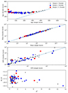 |
Fig. A.1. Comparison of the two SFHs used in the CIGALEfitting process: the single burst model (x-axis) and the double burst model (y-axis). These graphs include the highly-magnified object described in the main text and removed from the MS fitting. In descending order, the graphs depict the comparison of the age of the main stellar population, the stellar mass, the SFR, and the |

The SFR exhibits a higher dispersion when comparing the two SFHs, however, there is no significant offset. This greater dispersion in the SED-derived SFR is expected, as demonstrated in the above references, as well as in Mercier et al. (2022). This comes from the lack of data in the rest-frame mid and far infrared (MIR-FIR), which would be useful to constrain the dust content of these galaxies (although it is expected to be limited (De Barros et al. 2017; Goovaerts et al. 2023)).
A further check on the reliability of galaxy parameter estimation is performed using CIGALE’s mock catalogue function. This is a self-consistency check on derived physical parameters, inbuilt within CIGALE, which uses the best-fit parameters as truth values, creating an artificial catalogue and then adding noise drawn from the observed uncertainties. These artificial observations then undergo the same fitting process as the actual observations and a comparison of the artificial and best-fit parameters gives an indication of how well the physical quantities are retrieved. This comparison is shown in Fig. A.2. Altogether, these tests show that CIGALEcan reliably recover the relevant physical parameters of the LAEs for the estimation of the MS relation.
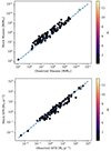 |
Fig. A.2. Results of the mock catalogue construction and fitting. Upper panel: Comparison of observed and mock stellar masses, colour-coded by the |


All Tables
All Figures
|
Fig. 1. Distribution of the 96 individual LAEs used in this study in redshift and absolute UV magnitude, colour-coded by lensing magnification. Redshifts quoted are spectroscopic from MUSE and magnitude values are derived from the filter that covers the rest frame 1500 Å emission. Horizontal dashed lines denote relevant limits: red denotes the MUV limit in an equivalent blank field study (Kusakabe et al. 2020) and black denotes the integration limit used when calculating the star formation rate density from the UV luminosity function (LF) in the latest study (Bouwens et al. 2022b). |
| In the text | |
|
Fig. 2. Stellar mass vs Lyman-α parameters. Left: stellar mass plotted against Lyman-α luminosity. Right: stellar mass plotted against EWLyα. Blue dashed lines indicate linear fits to the data and cyan shaded areas the 1σ uncertainties on the fits, details of which are given in the text. Median uncertainties on the Lyman-α parameters are shown by the horizontal black error bars. |
| In the text | |
|
Fig. 3. Stellar mass vs SFR: the galaxy MS. Upper panel: 96 LAEs in our final sample plotted on the star-forming MS, together with the best fits to the data of P23, S14 and the best fit to the LAEs following Eq. (1). LAEs are colour-coded by as ‘Time’, in Gyr, which is the age of the Universe at the observed redshift. The purple, dotted line indicates the lowest-stellar mass limit of S14’s review (2 × 10⁷ M⊙) and the green, dotted line indicates the lowest-stellar mass limit of P23’s review (6 × 10⁹ M⊙). The pink shaded area denotes the ±1σ area for the best-fit MS relation at the sample mean age, ∼1.48 Gyr. The mean error bars in three mass bins (106 < M/M⊙ < 2.5 × 10⁷, 2.5 × 10⁷ < M⋆/M⊙ < 5 × 10⁸ and 5 × 10⁸ < M⋆/M⊙ < 1010) are shown in black at the bottom of the plot. Lower: same LAEs and best-fit relation, but compared this time to the results in the same mass range that have been UV-selected, namely: the LBGs from A2744 from Goovaerts et al. (2023) as grey diamonds, with a blue best-fit relation, and the mass-binned results from S17 as coloured diamonds with error bars. |
| In the text | |
|
Fig. A.1. Comparison of the two SFHs used in the CIGALEfitting process: the single burst model (x-axis) and the double burst model (y-axis). These graphs include the highly-magnified object described in the main text and removed from the MS fitting. In descending order, the graphs depict the comparison of the age of the main stellar population, the stellar mass, the SFR, and the |
| In the text | |
|
Fig. A.2. Results of the mock catalogue construction and fitting. Upper panel: Comparison of observed and mock stellar masses, colour-coded by the |
| In the text | |
Current usage metrics show cumulative count of Article Views (full-text article views including HTML views, PDF and ePub downloads, according to the available data) and Abstracts Views on Vision4Press platform.
Data correspond to usage on the plateform after 2015. The current usage metrics is available 48-96 hours after online publication and is updated daily on week days.
Initial download of the metrics may take a while.