| Issue |
A&A
Volume 678, October 2023
|
|
|---|---|---|
| Article Number | A174 | |
| Number of page(s) | 13 | |
| Section | Cosmology (including clusters of galaxies) | |
| DOI | https://doi.org/10.1051/0004-6361/202347110 | |
| Published online | 18 October 2023 | |
Evolution of the Lyman-α-emitting fraction and UV properties of lensed star-forming galaxies in the range 2.9 < z < 6.7⋆
1
Aix-Marseille Université, CNRS, CNES, LAM (Laboratoire d’Astrophysique de Marseille), UMR 7326, 13388 Marseille, France
e-mail: This email address is being protected from spambots. You need JavaScript enabled to view it.
2
Department of Astrophysics, Vietnam National Space Center, Vietnam Academy of Science and Technology, 18 Hoang Quoc Viet, Hanoi, Vietnam
3
Graduate University of Science and Technology, VAST, 18 Hoang Quoc Viet, Cau Giay, Vietnam
4
Univ. Lyon, Univ. Lyon1, ENS de Lyon, CNRS, Centre de Recherche Astrophysique de Lyon UMR5574, 69230 Saint-Genis-Laval, France
5
Department of Astronomy, Oskar Klein Centre, Stockholm University, AlbaNova University Centre, 106 91 Stockholm, Sweden
6
7 Avenue Cuvier, 78600 Maisons-Laffitte, France
7
Department of Physics, ETH Zürich, Wolfgang-Pauli-Strasse 27, 8093 Zürich, Switzerland
Received:
6
June
2023
Accepted:
17
July
2023
Abstract
Context. Faint galaxies are theorised to have played a major role, perhaps the dominant role, in reionising the Universe. Their properties, as well as the Lyman-α emitter (LAE) fraction, XLAE, could provide useful insights into this epoch.
Aims. We used four clusters of galaxies from the Lensed Lyman-alpha MUSE Arcs Sample (LLAMAS) that also have deep HST photometry to select a population of intrinsically faint Lyman break galaxies (LBGs) and LAEs. We study the interrelation between these two populations, their properties, and the fraction of LBGs that display Lyman-α emission.
Methods. The use of lensing clusters allows us to access an intrinsically faint population of galaxies, the largest such sample collected for this purpose: 263 LAEs and 972 LBGs with redshifts between 2.9 and 6.7, Lyman-α luminosities in the range 39.5 ≲ log(LLyα)(erg s−1)≲42, and absolute UV magnitudes in the range −22 ≲ M1500 ≲ −12. In addition to matching LAEs and LBGs, we define an LAE+continuum sample for the LAEs that match with a continuum object that is not selected as an LBG. Additionally, with the use of MUSE integral field spectroscopy, we detect a population of LAEs completely undetected in the continuum.
Results. We find a redshift evolution of XLAE in line with literature results, with diminished values above z = 6. In line with past studies, we take this as signifying an increasingly neutral intervening intergalactic medium. When inspecting this redshift evolution with different limits on EWLyα and M1500, we find that the XLAE for the UV-brighter half of our sample is higher than the XLAE for the UV-fainter half, a difference that increases at higher redshifts. This is a surprising result and can be interpreted as the presence of a population of low Lyman-α equivalent width (EWLyα), UV-bright galaxies situated in reionised bubbles and overdensities. This result is especially interesting in the context of similar, UV-bright, low EWLyα objects recently detected during and around the epoch of reionisation. For intrinsically fainter objects, we confirm the previously observed trend of LAEs among LBGs as galaxies with high star formation rates and low dust content, as well as the trend of the strongest LAEs having, in general, fainter M1500 and steeper UV slopes.
Key words: gravitational lensing: strong / galaxies: high-redshift / dark ages / reionization / first stars
Tables 1 and 2 are available at the CDS via anonymous ftp to cdsarc.cds.unistra.fr (130.79.128.5) or via https://cdsarc.cds.unistra.fr/viz-bin/cat/J/A+A/678/A174
© The Authors 2023
 Open Access article, published by EDP Sciences, under the terms of the Creative Commons Attribution License (https://creativecommons.org/licenses/by/4.0), which permits unrestricted use, distribution, and reproduction in any medium, provided the original work is properly cited.
This article is published in open access under the Subscribe to Open model. This email address is being protected from spambots. You need JavaScript enabled to view it. to support open access publication.
1. Introduction
After the Dark Ages, the neutral gas in the intergalactic medium (IGM) was reionised: the last phase transition undergone by the Universe. This process ended with the hydrogen in the IGM ionised, around z = 6 (Fan et al. 2006; McGreer et al. 2015; Planck Collaboration VI 2020; Lu et al. 2022). There are two main candidates thought to be responsible for this process, star-forming galaxies (SFGs; Bouwens et al. 2015a; Finkelstein et al. 2015; Livermore et al. 2017) and active galactic nuclei (Madau & Haardt 2015; Grazian et al. 2018). The influence of active galactic nuclei is likely small (Onoue et al. 2017; Parsa et al. 2018; McGreer et al. 2018; Jiang et al. 2022). Currently, the favoured candidate is SFGs, particularly faint SFGs (Robertson et al. 2013; Bouwens et al. 2015b; Stark 2016), although the possibly significant contribution of bright SFGs is still debated (Naidu et al. 2020; Matthee et al. 2022).
One of the most powerful tools for studying these intrinsically faint SFGs is Lyman-α emission. Galaxies that exhibit Lyman-α emission are called Lyman-α emitters (LAEs). The strength of the Lyman-α line for equivalent widths (EWs) greater than, for instance, 25 Å allows us to identify intrinsically faint and/or high-redshift galaxies. In recent years, this has been exploited from several different angles in order to learn more about galaxies during this epoch as well as the state of the IGM and hence reionisation itself (see, for example, the reviews by Stark 2016; Dijkstra 2016, and Robertson 2022 and references therein).
Additionally, the use of lensing allows us to probe fainter galaxies than possible with blank field surveys, down to Lyman-α luminosities of ∼1039 erg s−1 (Bina et al. 2016; Smit et al. 2017; de La Vieuville et al. 2019, 2020; Richard et al. 2021; Claeyssens et al. 2022, the last four of which are henceforth dLV19, dLV20, R21, and C22). This gives us direct access to faint populations, which are currently the favoured candidates for the main contributor to reionisation. This avenue has been explored in recent studies with small to medium sample sizes (dLV20; Fuller et al. 2020). Lensing, however, comes with compromises on sample size and the volume of the Universe probed. Even more recently, samples of more significant sizes (hundreds of objects) have become available, such as the Lensed Lyman-alpha MUSE Arcs Sample (LLAMAS; R21,C22).
In order to investigate reionisation and the role of SFGs, the fraction of Lyman break galaxies (LBGs) that exhibit Lyman-α emission (henceforth referred to as the LAE fraction, or XLAE) is particularly interesting. The Lyman break is caused by the absorption of photons at wavelengths shorter than 912 Å by neutral hydrogen gas around the galaxy and up to 1216 Å by the Lyman forest along the line of sight. This can be used to search for galaxies photometrically using the ‘drop-out’ technique: galaxies will ‘drop out’ of filters bluewards of the Lyman break. Lyman-α emission is scattered by neutral hydrogen in the IGM, interstellar medium, and circum-galactic medium, so whether or not Lyman-α emission is detected from LBGs gives us information about the content of these media, in particular how ionised they are, which has the potential to help in reconstructing the timeline and scale of reionisation (see, for example, Mason et al. 2018b; Arrabal Haro et al. 2018; Kusakabe et al. 2020; Leonova et al. 2022; Bolan et al. 2022). Studies show a drop in the prevalence of LAEs among LBGs (XLAE) above z = 6, suggesting an increasing neutrality of the IGM before this time and supporting the established reionisation timeline (Stark et al. 2010, 2011; Pentericci et al. 2011, 2018; Caruana et al. 2014, 2018; De Barros et al. 2017; Hoag et al. 2019a; dLV20).
However, there are significant uncertainties associated with both the measurement of XLAE and its usage as a probe of the reionisation history. The evolution of XLAE with redshift could also be due to the inherent evolution of one or both of the populations considered, rather than solely a consequence of the changing state of the IGM (Bolton & Haehnelt 2013; Mesinger et al. 2015). Progress has been made in understanding the impact of the interstellar medium, circum-galactic medium, and dust attenuation on Lyman-α emission (Verhamme et al. 2008; Zheng et al. 2010; Dijkstra et al. 2011; Kakiichi et al. 2016); however, there is still significant debate about the physics of Lyman-α photon escape, in simulations as well as observations, at different redshifts and how this impacts LAE visibility and hence XLAE (Dayal et al. 2011; Matthee et al. 2016; Hutter et al. 2014; Sobral & Matthee 2019; Smith et al. 2022).
Additionally, XLAE has shown some dependence on the absolute rest-frame UV magnitude (Stark et al. 2010, 2011; Schaerer et al. 2011; Schenker et al. 2014; Kusakabe et al. 2020) and a significant dependence on the Lyman-α EW cut above which the XLAE is calculated (Stark et al. 2010; Caruana et al. 2018; Kusakabe et al. 2020). It is crucial to be aware of these factors when comparing results in the literature.
Equally important are the possible biases introduced by the different methods of selecting both the UV ‘parent sample’ and the LAE sample. When collecting the parent sample using the Lyman break, there is no standard way of selecting these galaxies. Some samples are selected via colour–colour cuts (for example, Stark et al. 2010; Pentericci et al. 2011; Bouwens et al. 2015a, 2021; Pentericci et al. 2018; Yoshioka et al. 2022), and some by photometric redshifts (Caruana et al. 2018; Fuller et al. 2020; Kusakabe et al. 2020; dLV20), although this probably does not have a large effect on the sample as the procedure to find the photometric redshift relies on the Lyman break in the same way as the colour–colour cuts (dLV20). The employed colour–colour cuts depend on the instrument and bands used to observe the sample as well as the depth of the observations, leading to different cuts for each study.
The exact selection process using photometric redshifts varies from study to study. For example, authors decide the signal-to-noise required for a detection as well as how to deal with the probability distributions provided by most photometric redshift codes.
The way the search for LAEs is conducted once the parent sample has been selected is not standardised either. Some authors select LAEs based on narrow-band (NB) photometry (Arrabal Haro et al. 2018; Yoshioka et al. 2022), some search for Lyman-α emission from UV-selected samples using multi-object slit spectroscopy (Stark et al. 2010, 2011; Pentericci et al. 2011, 2018; De Barros et al. 2017; Fuller et al. 2020), and some use integral field unit (IFU) spectroscopy (Caruana et al. 2018; dLV20; Kusakabe et al. 2020).
Using slit spectroscopy to search a UV-selected sample for Lyman-α emission can be problematic since the Lyman-α emission is not always centred on the UV emission; in fact, it has often been found to have an offset. C22 report a median offset of ΔLyα − UV = 0.66 ± 0.14 kpc, and Hoag et al. (2019b) find an offset corresponding to 0 25 at z = 4.5. Therefore, slit spectroscopy may not see the Lyman-α emission at all, or may miss some flux from extended emission.
The completeness of the different samples is also an important factor to take into account in these types of studies. Completeness is a correction made to the amount of objects observed to account for those present in the field but not observed. This correction depends on many factors and is different for each study. Several different approaches have been employed in the literature. Stark et al. (2010) determined the completeness of their Lyman-α detections by inserting fake emission lines across their spectra and attempting to detect them using the original detection process, a method that has evolved into the complex Lyman-α completeness treatments seen in IFU studies such as Kusakabe et al. (2020) and dLV20. dLV20 and this study use the extra complication engendered by lensing fields (see dLV20 and Thai et al. 2023). dLV20 show that the inclusion of the LAE completeness correction is important for the calculation of XLAE.
The study can be performed on a UV-complete subsample of the LBG population as in Kusakabe et al. (2020), but it is common to assume that one’s LBG selection is highly complete for the signal-to-noise requirements imposed in the selection process. This is also an assumption sometimes made for the Lyman-α selection. For studies not involving lensing, one can easily calculate the apparent magnitude at which a sample becomes incomplete in the UV selection at the 10% and 50% level, as in Arrabal Haro et al. (2018).
In light of these discrepancies between different studies, it is not surprising that there is significant disagreement on the precise values and evolution of XLAE. There is only a general consensus that XLAE rises from lower redshifts to a redshift of ∼6, after which it decreases (see, among others, Pentericci et al. 2011; Stark et al. 2011; De Barros et al. 2017; Arrabal Haro et al. 2018; Caruana et al. 2018; Fuller et al. 2020; dLV20).
In addition to the reasons previously mentioned, the scatter in the results from these various studies can come from issues related to sample size as well as the exact sample used to calculate the fraction. For example, the inclusion limits on M1500 are not homogeneous across all studies, nor are the inclusion limits on the Lyman-α EW.
In this paper we investigate faint SFGs towards the epoch of reionisation (2.9 < z < 6.7) observed behind four lensing clusters in the Hubble Frontier Fields (HFF; Lotz 2017), specifically chosen for being efficient enhancers of such high-redshift objects. We selected LAEs from Multi-Unit Spectroscopic Explorer (MUSE) IFU spectroscopy and LBGs using deep Hubble photometry and photometric redshifts. We present the largest combined LAE and LBG sample of lensed, intrinsically faint galaxies used for this purpose to date. Our sample reaches as faint as M1500 ∼ −12 and log(LLyα/erg s−1)∼39.5 after correcting for lensing magnification. This is similar to the latest LBG selection in the HFF from Bouwens et al. (2022). Having blindly selected these populations of galaxies, we compare their UV and Lyman-α-derived properties and explore the fraction of LAEs among the LBG population, its redshift evolution, and its UV magnitude dependence.
In Sect. 2 we cover the data from MUSE and the HFF as well as the specific selection criteria we apply for our samples of LAEs and LBGs. We outline the photometric redshifts used and the blind matching of both populations. Section 3 outlines our results pertaining to derived properties: EWs, UV slopes, and star formation rates (SFRs), as well as the interrelation between the two populations, including several approaches for determining the fraction of LAEs among the LBG population. We discuss the implications for reionisation and the properties of these high-redshift galaxies. In Sect. 4 we summarise our findings and offer perspectives for future surveys.
The Hubble constant used throughout this paper is H0 = 70 km s−1 Mpc−1, and the cosmology is ΩΛ = 0.7 and Ωm = 0.3. All EWs and UV slopes are converted to their rest-frame values, and all magnitudes are given in the AB system (Oke & Gunn 1983). All values of the UV absolute magnitude (defined at the 1500 Å rest frame, M1500) and Lyman-α luminosities are given corrected for magnification.
2. Data and population selection
For this study, we combined MUSE (Bacon et al. 2010) IFU observations with the deepest Hubble Space Telescope (HST) photometry available in lensing clusters. The HFF clusters (Lotz 2017) are ideal for this work, specifically, we use Abell 2744, Abell 370, Abell S1063, and MACS 0416 (henceforth A2744, A370, AS1063, and M0416). The MUSE observations of these clusters are taken from the data collected in R21, from which the LAEs are selected to form the LLAMA Sample (C22). The complementary HST data are from the HFF-DeepSpace Program (PI: H. Shipley)1.
2.1. MUSE LAEs: LLAMAS
2.1.1. LAE selection
The MUSE data we use for this work is part of LLAMAS (C22). These observations were part of the MUSE Guaranteed Time Observing programme and are comprehensively described in C22 as well as R21. The catalogues and lens models for the four clusters used in this work are available online2 and at the CDS. We summarise here the details of the reduced MUSE datacubes and the LAE selection process.
The MUSE datacubes contain the flux and variance over a 1 × 1 arcmin2 field of view, with spatial and spectral pixel scales of 0.2″ and 1.25 Å. The spectral range covers 4750 Å–9350 Å, allowing the detection of Lyman-α between redshifts of 2.9 and 6.7. Integration times on the clusters we use for this work vary between 2 and 14 h, with different pointing configurations (see below). The clusters are all in the range 0.3 < z < 0.4, providing magnifications useful to amplify sources in the MUSE Lyman-α redshift range. Details of the four clusters are given in Table 1. Full details covering all 17 LLAMAS clusters can be found in C22 and Thai et al. (2023).
Details of each lensing cluster used in this study.
In order to detect line emission sources such as LAEs, R21 follow the prescription laid out in Weilbacher et al. (2020), using the MUSELET software (Piqueras et al. 2019)3, which is used on MUSE NB images. Subsequently, the Source Inspector package (Bacon et al. 2023) is used to identify sources and assign their redshifts. This package allows users to cycle through a list of sources with all the relevant information: spectra, NB images, HST counterparts, MUSELET results, and redshift suggestions. With this information, users can decide on a redshift for an object as well as assigning each source a redshift-confidence level from 1 to 3. A confidence level of 1 denotes a tentative redshift and a confidence level of 3 denotes a redshift with a high confidence. For this study we only use LAEs with confidence levels of 2 and 3, indicating secure redshifts. In our sample – A2744, A370, AS1063, M0416 – there are 263 such LAEs.
Magnifications of sources are assigned with the use of the parametric mass distribution models in R21 (for A2744, A370 and M0416, for AS1063, the lens model comes from Beauchesne et al. 2023) and the LENSTOOL software (Kneib et al. 1996, 2011; Jullo et al. 2007; Jullo & Kneib 2009). These models are well constrained by the large number of multiple images with strong spectroscopic redshifts (levels 2 and 3 as described above) in these clusters. R21 estimate a typical statistical error of 1% of the mass profile of these clusters. The models in turn give the magnifications of the sources used in this study, which range from 0.8 (de-magnified) up to 137. Most sources have magnifications between 1.5 and 25. While these lensing models are well understood and benefit from many multiple image systems as constraints, small systematic uncertainties related to the lens model used can still persist due to the particular choice of mass distribution (see, for example, Meneghetti et al. 2017; Acebron et al. 2017, 2018; Furtak et al. 2021).
2.1.2. LAE flux determination
The Lyman-α flux for the LAEs in our sample was extracted using one of two different methods.
The main method employed in the LLAMA Sample is the line profile fitting procedure described in C22. For the subsample used in this work (263 LAEs), all those behind A2744 and 20 behind the other three clusters (roughly half the subsample), we use a method involving SExtractor (Bertin & Arnouts 1996) following the procedure outlined in dLV19. We give a brief description of both methods.
The line profile fitting method utilises three steps: spectral fitting, NB image construction and spectral extraction. The first step involves fitting an asymmetric Gaussian function to the Lyman-α peak with the EMCEE package from Foreman-Mackey et al. (2013), using 8 walkers and 10 000 iterations (in double peaked cases, both peaks are considered separately and their fluxes combined after the extraction is complete). The peak position of the Lyman-α line, flux, full width at half maximum, and asymmetry of the source are all fitted. The second step takes the result for the peak position and creates a NB image around the LAE. The continuum around the LAE in redward and blueward bands of width 24 Å is subtracted from the Lyman-α flux. The NB bandwidth is optimised such that the S/N of the Lyman-α peak is maximised in an aperture of radius 0.7″. Finally, utilising this new NB image of the LAE, a new extraction is performed from the MUSE datacube, ensuring that as much of the Lyman-α emission from the galaxy and surrounding halo is extracted. The process is repeated twice more, each time using the latest NB image and extraction.
The second method is employed for A2744 and in the three other clusters for the cases where the first method fails to fit the Lyman-α flux. This happens in very low signal-to-noise cases or sources close to the edge of the datacube. This method uses SExtractor on NB images as described in dLV19. The NB images in question are those in which each LAE is detected. Three sub-cubes are extracted from the main datacube, one encompassing the Lyman-α emission and two either side of it (spectrally) each of width 20 Å. These cubes are averaged to form a continuum image, which is subtracted pixel-by-pixel from an image formed by averaging the cube containing the Lyman-α emission. SExtractor is then run on this new continuum-subtracted image and the FLUX_AUTO parameter is used to estimate the fluxes of the LAEs. To deal with faint sources or those with an extended, low surface brightness, SExtractor can progressively loosen the detection conditions (using the DETECT_THRESH and DETECT_MINAREA parameters) so that a flux can also be extracted for these sources.
Figure 4 of Thai et al. (2023) shows the comparison between the two methods of extracting the Lyman-α flux. In general, the two methods agree well. In some cases, the line profile fitting method estimates a larger flux due to its enhanced appreciation of the line complexity.
In Fig. 1 we show the properties of our sample of LAEs in red. In order to have a similar derivation of M1500 for all our LAEs, regardless of detection in HST photometry, values of M1500 are calculated from the filter closest to the 1500 Å rest frame wavelength (where available, and the 2σ upper limit of the continuum taken from this filter where not), and corrected for magnification. Lyman-α luminosities are derived from the fluxes described above and also magnification-corrected. In terms of Lyman-α luminosity we probe roughly between 39.5 < log10(LLyα/erg s−1) < 42.5, with decreased statistics near the faintest and brightest limits. This faint population can at present only be accessed with lensing clusters; the typical limit in blank fields lies around log10(LLyα) ∼ 42 (see, for example, Herenz et al. 2019), down to log10(LLyα)∼41.5 in the MUSE Ultra Deep Field (Drake et al. 2017).
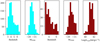 |
Fig. 1. Redshift and M1500 (and Lyman-α luminosity for the LAEs) distributions of the two samples used in this work. LBGs are shown in blue and LAEs in red. |
2.2. HFF data
The HST observations of the clusters used in this work are from the Hubble Frontier Fields programme (ID: 13495, P.I: J. Lotz). In particular, we use the photometric catalogues of the HFF-DeepSpace Program (Shipley et al. 2018). As part of this programme, the authors collected homogeneous photometry across the HFF, including deep KS-band imaging (2.2 μm) from the HAWK-I on the Very Large Telescope (VLT) and Keck-I MOSFIRE instruments Brammer et al. (2016). Additionally included are all available data from the two Spitzer/IRAC channels at 3.6 μm and 4.5 μm. The two Spitzer/IRAC channels at 5.8 μm and 8 μm were judged to be too noisy and excluded from the spectral energy distribution (SED) fitting process (see Sect. 2.3). The details of the filters used, and their depths, for each cluster can be found in Table 2. The bright cluster galaxies and intra-cluster light are subtracted by Shipley et al. (2018) for improved photometry of background sources in these very crowded fields. The detection image for each of these clusters is made up of a combination of the F814W, F105W, F125W, F140W and F160W bands (point-spread-function-matched to the F814W band), after the modelling out of the bright cluster galaxies.
5σ limiting magnitudes of each filter for the four clusters.
The area that MUSE observed for each of these clusters is fully contained within the HST area, so we cut the HST area we consider to that of the MUSE data. The resulting effective (lens-corrected) co-volume, derived from LENSTOOL source-plane projections, is 22 910 Mpc3 over the redshift range 2.9 < z < 6.7.
2.3. LBG selection
We calculate photometric redshifts and probability distributions (hereafter P(z)) in order to perform our LBG selection. We use the package New-Hyperz (Bolzonella et al. 2000) to estimate redshifts and probability distributions. This package uses a standard χ2 minimisation technique to fit template galaxy SEDs to photometric data points. It has been optimised for the redshift determination of high-redshift galaxies so is ideal for our purpose. We use a suite of template spectra to fit the photometric data: the four template spectra from Coleman et al. (1980), two Starburst99 models with nebular emission (Leitherer et al. 1999): a single burst model and a constant SFR model (where each spans five metallicities and 37 stellar population ages), and seven models adapted from Bruzual & Charlot (2003). Included in these seven are a star formation burst model, five exponentially decaying models with timescales between 1 and 30 Gyr and a constant star formation model. The redshift range we use in New-Hyperz is 0–8 with a step in redshift of 0.03. The Calzetti extinction law (Calzetti et al. 2000) is used to account for internal extinction with values of Av allowed to vary between 0 and 1.5 mag. No priors on galaxy luminosity were introduced during this process, avoiding any bias introduced by lensing magnification.
For a galaxy to be included in the LBG sample for this study we demand that the best solution for the photometric redshift lies in the range 2.9 < z < 6.7. We also accepted any candidates not in this range that have 1σ errors overlapping with it. In practice, this accounts for just 14 objects. To make sure the detection is real, we also demand a 5σ detection in at least one HST filter. New-Hyperz provides a redshift probability distribution, P(z), which can have two peaks, in which case there are two redshift solutions for that particular galaxy. We accept galaxies into the sample if only one of the peaks is in the required range, as long as 60% of the integrated P(z) also lies in this range. We can compare the photometric redshift results for those objects also selected as LAEs to the spectroscopic redshift determined from the peak of the Lyman-α emission. Figure 2 shows this comparison. The dashed lines indicate regions constrained by |zspec − zphot|< 0.15(1 + zspec) and |zspec − zphot|< 0.05(1 + zspec). We encode the apparent magnitude in the F125W filter in the colour bar to demonstrate that the instances in which New-Hyperz performs poorly (i.e., instances outside of the outer region specified above) tend to be fainter objects with magnitudes ≳28.
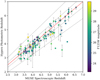 |
Fig. 2. Photometric vs. spectroscopic redshift comparison of objects selected as LAEs and LBGs. The red line indicates the one-to-one relation, and the dashed black lines indicate the typical error bounds of |zspec − zphot|< 0.15(1 + zspec) and |zspec − zphot|< 0.05(1 + zspec). Almost all of the photometric redshifts agree with their spectroscopic equivalents within the outer of these two bounds. Those that do not tend to be fainter objects, with magnitudes of 28 and above. |
Finally, we manually inspect our LBG sample using the HST images, photometry, SED fitting from New-Hyperz and the LENSTOOL package with the lens models described in Sect. 2.1.1. This procedure is designed to identify multiple images in the LBG sample caused by the gravitational lensing, as well as to remove any obvious spurious detection; regions of noise or contamination erroneously selected as LBGs. Multiple images are identified using a combination of LENSTOOL predictions, redshift determinations and SEDs from New-Hyperz, and visual inspection of the HST images. LENSTOOL predictions, redshift estimates and colours of objects have to match for those objects to be designated a multiple image system. The colours used are F814W − F606W, F105W − F814W, F140W − F105W, all of which have to match to within 2σ for the objects in question to be designated multiple images. From each system, a representative LBG image is chosen. This image is the least contaminated, or, in the case of a match with an LAE multiple image system, the image chosen to represent the LBG multiple system matches the selected LAE image (see Sect. 2.4).
2.4. Matching populations
Having blindly selected our LAE and LBG samples, we compared them, using a matching radius of  , to see which objects are selected as both. The results are shown in Table 1.
We selected a population labelled LAE+continuum, which denotes objects that are selected as LAEs, for which we see a continuum in the HST images, but where this continuum fails to meet the selection criteria for our LBG sample. Mostly, these galaxies fail on the S/N criteria outlined in the previous subsection, indicating a faint continuum or a noisy area in the HST images. Nevertheless, we kept these objects as, thanks to the Lyman-α emission, we know that there is a high-redshift galaxy at these positions. In the previous work of this nature solely on A2744, dLV20 simply included these objects in the LAE+LBG sample, relaxing the signal-to-noise criterion for these objects, seeing as the presence of an object (as well as its redshift) was known thanks to the Lyman-α emission. Here, however, we kept the distinction between these continuum detections with Lyman-α emission and the LBGs in our sample that fulfil all the criteria laid out in the previous subsection. Details on the inclusion of this sample in the analysis of the LAE fraction, XLAE, are given in Sect. 3.2.1.
For the LAEs, a ‘best’ image is chosen, a process described fully in Thai et al. (2023). This allows us to choose representative images that are minimally impacted by neighbours and have high signal-to-noise and moderate magnification. When selecting LBGs, we kept the image corresponding to the best LAE image selected by Thai et al. (2023) where possible. However, in some cases we chose another image, because that particular LAE image is selected as LBG rather than continuum only. We ensure that the image chosen is always of similar quality. A modification of this nature is rare and we impose it in fewer than ten systems across the whole LAE sample. The original Lyman-α flux and magnification of the source, as given in the LLAMAS catalogues, is used for our analysis on the properties of these objects; however, their designation as LAE+continuum or LAE+LBG can change based on this.
2.5. Completeness determination
As covered in Sect. 1, the completeness of the populations considered in such a study is very important. This correction to the number of sources detected aims to reflect the number of sources that are missed in the detection process and thus the number of sources actually present in the field of view.
The completeness methods used for the LAEs in this work are described in Thai et al. (2023) and summarised here. Following the procedure first laid out in dLV19, sources are treated individually in this computation. Each source’s brightness distribution profile, both in the spatial and spectral dimensions, is modelled and randomly injected 500 times into the NB layer of the original MUSE datacube where its Lyman-α emission reaches a maximum. This process is performed in the image plane, in order to recreate as closely as possible the actual process of detection with MUSELET. The completeness of the source is the number of times (out of 500) it is successfully detected and extracted.
Since it is the local noise that likely decides whether or not such an injected source is detected, to account for variations in the local noise, Thai et al. (2023) change the size of the NB image used to re-detect the simulated sources from 30″ × 30″ to 80″ × 80″. This was found to improve the extraction of the source when that source has close neighbours. The mean completeness value found for our sample is 0.72 and the standard deviation is 0.34.
Finally, each source’s contribution to the LAE fraction is corrected by a value 1/Ci, where Ci is the completeness value of that source. In effect, a source with a completeness value of 0.5 contributes two LAEs to the calculation of the LAE fraction.
3. Results
3.1. UV properties of the populations
In order to ascertain the similarities and differences between our populations of high-redshift galaxies, it is useful to look at the physical properties we derive from the HST photometry and their relation to Lyman-α emission. This can also help disseminate how these properties tie in with the LAE fraction (see Sect. 2.1.2). Additionally, we can appraise any differences from the established trends for these high-redshift galaxies that may appear in our sample of faint, lensed galaxies.
To evaluate this relation to Lyman-α emission, the Lyman-α equivalent width, EWLyα, is an important property to derive. We can then compare this to UV-derived properties. In order to calculate EWLyα values for our sample, first we derive UV slopes by fitting the photometric points starting above the location of the Lyman-α emission (irrespective of whether or not we detect it for a given galaxy) and including all the filters up to 2600 Å in the rest-frame, adapting the approach used in Castellano et al. (2012), Schenker et al. (2014), Bouwens et al. (2015a). We fit a power law, Fλ ∝ λβ, where β is the UV slope, to the photometry. We chose this method as it does not rely on SED fitting with a set of templates that have specific allowed values of β.
Subsequently, by using this photometrically fitted UV slope for each object, we can ascertain the continuum flux level beneath the Lyman-α emission. Hence, we calculated the Lyman-α equivalent width (EWLyα) by dividing the Lyman-α flux by the continuum flux level, corrected to its rest-frame level. In this process we take into account the error on the UV slope resulting from the fitting process, as well as the error associated with the Lyman-α flux (see Sect. 2.1).
For the objects with no associated continuum, the upper limits of the continuum are taken from the filter closest to the 1500 Å rest-frame emission. For the objects with no associated Lyman-α emission, the detection limits of the Lyman-α emission are used.
The EW distribution with redshift for all our sample is shown in Fig. 3. The dashed black line denotes the typical EW inclusion limit for objects to the calculation of XLAE (see Sect. 3.2.1). The percentage of objects above this limit is 44% and 50% for LAE+LBG objects and LAE+continuum objects, respectively. This is to be expected as the objects selected as continuum but not LBG are in general fainter, giving rise to higher values of EWLyα.
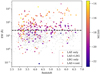 |
Fig. 3. Lyman-α EW (EWLyα) distribution for all our samples. Objects selected as LAEs or LBGs are denoted by larger stars, LAE+continuum by smaller stars, LAE-only by upward pointing triangles, and LBG-only by downward pointing triangles. EWLyα values for the latter two populations are calculated using the upper limits of the continuum and Lyman-α flux, respectively. The objects are colour-coded by M1500. The horizontal dashed line demarcates the 25 Å level, above which LAEs are included in the calculation of the LAE fraction. Error bars are omitted for clarity, but shown in Figs. 4 and 5. |
In Fig. 4 we compare EWLyα to UV magnitude for our LAE+LBG sample. UV absolute magnitude, M1500, is calculated from the filter closest to the 1500 Å rest-frame emission. We see a rise in EWLyα towards fainter M1500, in agreement with results reported in Stark et al. (2010), De Barros et al. (2017), Kusakabe et al. (2020). We note that above M1500 = −16 this graph is populated by high EW, continuum-undetected LAEs (shown by orange triangles). We did not include these objects in the binned averages as they are not LBGs and the continuum values are estimated upper limits; however, these objects indicate that this trend in EW likely increases to even fainter magnitudes than is populated by our current LBG selection. As the spatial extent of Lyman-α emission correlates with the size of the galaxy and hence M1500 (Wisotzki et al. 2016; Leclercq et al. 2017; C22), the trend in Fig. 4 is often seen as a natural result.
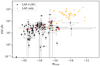 |
Fig. 4. EWLyα distribution over the range of UV absolute magnitude probed for the LAE+LBG sample. The red stars indicate the average in five equal-size bins between M1500 = −20 and M1500 = −15, the region that is well populated. De Barros et al. (2017) provide a similar plot (at z = 6) for a brighter sample with a similar rising average EWLyα. Our plot extends several magnitudes fainter, and we see that this trend continues down to at least M1500 = −16. An idea of the region fainter than M1500 = −15 can be gained by including the LAE-only sample (orange triangles), the vast majority of which are very faint in UV magnitude, and high-EWLyα objects. For these objects, EW error bars, coming only from the error on the Lyman-α flux, are smaller than the size of the points. The continuum values used are 2σ upper limits estimated from the filter that would see the emission at 1500 Å rest frame. |
We also compared EWLyα to the UV slope (Fig. 5). In general, high-EW LAEs are found to have bluer slopes (Stark et al. 2010; Schenker et al. 2014; De Barros et al. 2017). We report a slight increase (< 1σ) in average EW in bins between β = −1.0 and β = −3.0. However, similarly to De Barros et al. (2017), we find EWLyα values as high as ∼ 100 Å across the sample.
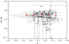 |
Fig. 5. UV slope plotted against EWLyα for the LAE+LBG sample. Orange dots represent UV slopes that, upon inspection, we find to be dubious: photometry that locally does not represent the slope well or has large errors. Red stars represent average values in equally sized bins between β = −3.5 and β = −1.0. The change in EWLyα across this range is not as significant as the change across the range of probed UV magnitudes (see Fig. 4); however, we see a lightly rising trend in EWLyα with bluer slopes down to β = −2.5. |
We derive SFRs from Lyman-α (SFRLyα) and from the UV continuum (SFRUV), based on the relations given in Kennicutt (1998) and the factor of 8.7 between L(Hα) and L(Lyα), assuming a Salpeter IMF (Salpeter 1955) and constant star formation. SFRLyα is a good lower limit on the intrinsic SFR as Lyman-α flux can be lost due to dust attenuation or a more or less opaque IGM (Zheng et al. 2010; Gronke et al. 2021). However, due to the use of an IFU, slit losses have no impact on the Lyman-α flux.
We compare the two measures of SFR for our LAE+LBG sample in Fig. 6, plotting the line of one to one ratio and the actual median ratio (SFRLyα/SFRUV) found in our sample. This median ratio (0.35), is well below the one to one ratio, indicating that in most cases the escape fraction of UV photons (the fraction of photons at 1500 Å rest frame that escape the galaxy), fesc, UV, exceeds that of Lyman-α photons (the fraction of Lyman-α photons that escape the galaxy), fesc, Lyα. This is less apparent in UV-fainter objects, where there is a greater fraction above the fesc, UV = fesc, Lyα line. This result is in line with previous findings in Ando et al. (2006), Schaerer et al. (2011) and dLV20. The explanation offered previously by Ando et al. (2006) and dLV20 relates to the likely difference between the UV-bright and UV-faint galaxies. If the UV-bright galaxies have had more time to evolve than UV-fainter objects, it is likely that they are chemically more complex and have a larger amount of dust. This would decrease the escape of Lyman-α photons and hence result in a smaller measured SFRLyα. We return to this point having compared the LAE fraction for the UV-bright and UV-faint halves of our sample in Sect. 3.2.1.
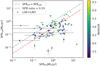 |
Fig. 6. Comparison of the derived SFRs for our LAE+LBG sample, colour-coded by redshift. The errors on the SFRLyα are smaller than the size of the points in most cases. The dashed blue line denotes a one-to-one SFR ratio, i.e., SFRUV = SFRLyα. Galaxies along this line also have equal escape fractions: fesc, UV = fesc, Lyα. Most of our sample lies under this line, and the dashed red line denotes the median SFR ratio of our sample, 0.35. For fainter objects with SFRUV < 1 M⊙ yr−1, a greater fraction lie above the line of equal SFR, a trend previously observed in Ando et al. (2006), Schaerer et al. (2011), and dLV20. |
Subsequently, we compare M1500 and SFRUV to the UV slopes of both samples (LBG and LAE+LBG) between −3.0 < β < −1.0: Fig. 7. In this graph, we calculate binned averages as in Figs. 4 and 5. However, for this plot the averages are computed for bins of equal population. For the LBG-only sample, there is a slight increase in SFRUV with steeper UV slopes, this is to be expected as steeper values of β generally indicate populations that are more intensely star forming.
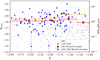 |
Fig. 7. M1500 and SFRUV vs. UV slope. The sample selected as LBG-only is shown in grey, and the LAE+LBG sample is colour-coded by redshift. Binned averages in SFRUV for the LBG and LAE+LBG samples are shown with red circles and golden squares, respectively. Each bin contains an equal number of the respective samples, and the horizontal error bars show the width (in terms of β) of each bin. Errors on the LBG-only objects are omitted for readability, and we note that there are LBG-only objects (and four LAE+LBG objects; see Fig. 5) that extend beyond the β limits of this graph; however, they are objects for which the calculation of the UV slope is uncertain. There are LBG-only objects that extend beyond the M1500 limits of the graph, but these are taken into account when computing the binned averages. |
From the binned averages we can see that for the population also selected as LAEs, the galaxies are distributed towards higher values of SFRUV and steeper UV slopes. This result supports previous findings (in various redshift ranges, as well as in simulations) that LAEs are in general dust-poor and are more intensely star forming than objects only selected as LBGs (Verhamme et al. 2008; Hayes et al. 2011, 2013; Sobral & Matthee 2019; Santos et al. 2020).
We extend this genre of analysis to our large sample of intrinsically faint galaxies, finding the same trends; LBGs also selected as LAEs have on average higher SFRUV and steeper UV slopes. High-EWLyα objects are on average fainter in absolute UV magnitude with steeper UV slopes, and those fainter in UV absolute magnitude tend to have fesc, Lyα approaching fesc, UV or in some cases above, while this is not seen for UV-brighter LAEs. All these trends are seen with significant scatter, which is to be expected given the intrinsically faint nature of the sample, the limits of the photometry (although it is the deepest available), and those objects that have a complex star formation history and physical structure, for which our assumption of constant star formation is less valid. Combined, our results reinforce the picture of high-redshift LAEs as UV-faint, intensely star forming, dust-poor galaxies and show that these trends hold for galaxies down to M1500 ∼ −12.
3.2. The interrelation between the LAE and LBG populations
We define four samples: objects identified as LBG-only, objects identified as LAE-only, objects identified as both LAE and LBG (LAE+LBG), and objects identified as LAE that have a continuum detected in the photometry from HST that does not meet our criteria for the LBG sample (LAE+continuum). These samples have 872, 55, 100, and 108 members, respectively.
The sample is dominated by A2744, with 46% of the LAEs and 35% of the LBGs; this is a large field of view with long MUSE exposures (see R21, C22, and Thai et al. 2023). However, as many fields of view as possible are valuable additions to the sample. The redshift distribution and the M1500 distribution of the sample are displayed in Fig. 8. We find the same result as dLV20 when considering the relative importance of LAEs that are totally undetected in the continuum. Their increasing presence is clear when looking at the faint region of the M1500 distribution, even when using the deepest HST photometry. This is crucial to note for any study wishing to catalogue the contribution to reionisation of all star-forming objects at high redshifts. This effect is naturally expected to strengthen with decreasing depth of photometry.
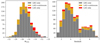 |
Fig. 8. M1500 distribution of the populations (left) and redshift distribution of the populations (right). The sample labelled ‘LAE+continuum’ includes all LAEs matched with continuum objects and LBG-selected galaxies. |
3.2.1. LAE fraction
Before discussing XLAE and its relevance to reionisation, we first outline what is typically meant by XLAE. The typical qualitative interpretation is ‘the fraction of UV-selected LBGs that display Lyman-α emission’. This stems from the technique of spectroscopic follow-up on a photometric preselection of targets (e.g., Stark et al. 2010, 2011). In the case of this study, both LAE and LBG selections are performed blindly. With an IFU, we also detect LAEs that have no continuum counterpart, objects that would clearly be missed in the aforementioned type of study.
Additionally, limits are typically placed on the inclusion of objects when calculating XLAE. The most common limits are EWLyα > 25 Å and M1500 > −20.25 (Stark et al. 2011; Schenker et al. 2014; De Barros et al. 2017; Mason et al. 2018b; Pentericci et al. 2018; Arrabal Haro et al. 2018; dLV20 among others); however, Caruana et al. (2014) use a limit of 75 Å. Other authors, such as Stark et al. (2010), Cassata et al. (2015), Caruana et al. (2018), Kusakabe et al. (2020), and Fuller et al. (2020), investigate different EW and M1500 or apparent magnitude ranges to assess the EW and UV magnitude evolution of XLAE, with the exact ranges depending on the study: the depths available and whether or not lensing is involved. In blank fields, most commonly authors investigate the bright and the faint halves of their sample, split at M1500 = −20.25 (e.g., Cassata et al. 2015; De Barros et al. 2017; Arrabal Haro et al. 2018). Alternatively, where sample sizes allow, studies bin results in M1500 from −22 to −18 (e.g., Caruana et al. 2018; Kusakabe et al. 2020). These are important distinctions to be aware of when comparing results from the literature. This discrepancy between the exact inclusion limits studies use, as well as the observational differences (as covered in the introduction) is likely a significant factor in the ongoing debate over the exact evolution of XLAE with redshift, EWLyα and M1500 (see Fig. 9).
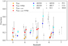 |
Fig. 9. LAE fraction, XLAE, over a redshift range of 2.9–6.7, using the typical literature limits of EWLyα > 25 Å and M1500 > −20.25. The coloured circles represent XLAE when just LAE+LBG objects are taken into consideration, and the coloured stars represent the same calculation but including the LAE+continuum sample (see Sect. 2.4). Coloured stars indicate these XLAE values including the completeness correction for the number of LAEs (see Sect. 2.5). Blue and cyan squares represent the results from dLV20, with cyan representing those with the completeness correction. Shorthand is used in the legend for the literature results, but we give the full list here (in the same order as the legend): Kusakabe et al. (2020), Arrabal Haro et al. (2018), De Barros et al. (2017), Stark et al. (2011), Pentericci et al. (2011), Cassata et al. (2015), and Mason et al. (2018b). A small redshift offset is artificially applied to some points for clarity. |
In this work we provide a perspective based on blind selections of both populations with an IFU and deep photometry with which we can assess more fully the landscape of these high-redshift galaxies. We compare the inclusion of objects only selected as LBG as well as the LAE+continuum sample described in Sect. 2.4. Given that we detect LAEs with no continuum counterpart we also discuss the effect this has on XLAE. We investigate different M1500 and EWLyα inclusion limits to provide context on the differing results in the literature. This last point is additionally motivated by the use of lensing fields in this study, meaning that we effectively probe a different population than blank field studies. It is therefore appropriate to investigate different regions of the EWLyα and M1500 space.
In Fig. 9 we compare our results to results from the literature in the classical manner with inclusion limits of M1500 > −20.25 and EWLyα > 25 Å. The redshift bins used are 2.5 < z < 3.5, 3.5 < z < 4.5, 4.5 < z < 5.5 and 5.5 < z < 7.0. For each bin, we include four values of XLAE: the fraction of LAEs among LBGs (yellow dots), the fraction of LAEs among LBGs with the completeness corrections described in Sect. 2.5 (red dots) and the same two measurements including the LAE+continuum objects (yellow and red stars; see Sect. 2.4).
Despite significant uncertainties, we see roughly the same trend as many results in the literature, with XLAE decreasing around z = 6. The decrease of XLAE shown in our data is quicker than many equivalent measurements in the literature. If one carries forward the assumption that XLAE efficiently probes the neutral hydrogen content, this result suggests that the IGM quickly becomes neutral after z = 6.
The objects we detect only as LAEs (making up ∼21% of our LAE sample) would push these fractions higher, were they to be included. Considering that these objects are extremely faint in terms of UV magnitude and high in terms of EWLyα, they would make an appreciable difference in the calculation of the fraction (in a similar way to the LAE+continuum sample shown by red and yellow stars in Fig. 9). There is little reason to suspect that with deeper photometry in the region that sees the rest frame UV emission, the continuum would remain undetected for these objects.
The high values of XLAE that we see in the first (low-redshift) bin in Fig. 9 are likely due to the fact that the Lyman break is harder to detect at these redshifts given the filters at our disposal. In order to check this, we perform a simulation, creating 100 000 fake LBG sources using Starburst99 templates (Leitherer et al. 1999). We add realistic noise to the data and spread them equally throughout the redshift and UV magnitude space probed by our study. We then attempt to select LBGs following the original selection criteria laid out in Sect. 2.3. In the first redshift bin (2.5 < z < 3.5) the amount of LBGs selected versus the number of simulated LBGs is drastically lower than the other bins, at < 10%. It is worth noting that this simulation was computed for AS1063: a ‘best-case scenario’, given that AS1063 has the most filters available in the short wavelength range ( < 606 nm). For sources at redshifts between 2.5 and 3, the break would appear between ∼320 nm and ∼365 nm. The blue filters have a shallower depth (for AS1063, F225W, F275W, F336W, and F390W have 5σ limiting magnitudes ∼24.0, 25.9, 26.3, and 25.4, respectively) than the redder HST filters and due to this and their scarcity (A2744 only has F275W and F336W), we struggle to recover all the LBGs in this bin (for complete filter depth information, see Table 2). This can also explain why in Fig. 1 we can see a trough in the distribution at the lower end of our redshift range, why XLAE is higher than many literature estimates in the lowest-redshift bin and forms part of the reason why we see little evolution between redshifts of 3 and 5. However, our results are still in agreement with the literature results at 1σ. Effects like this are not unexpected considering the varying nature of LBG (and LAE) selection.
The errors on XLAE as displayed in Figs. 9 and 10 contain several components. As mentioned, there is a big impact on sample inclusion from the EWLyα limits of 25 Å. Therefore, it is important to quantify an error based on this. We performed 1000 Monte Carlo trials of XLAE, sorting the EWLyα values in their error bars, assumed to be Gaussian. We evolved an error estimate for XLAE based on the 16th and 84th percentile of the resulting range of results for XLAE.
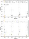 |
Fig. 10. Redshift evolution of XLAE in the bright and faint populations, split at M1500 = −18. The bright and faint populations are shown in blue and orange, and the completeness corrections in grey scale with the bright population in darker grey. The top panel corresponds to LAEs with EWLyα > 25 Å, while the lower panel shows the results when this limit is removed. The absence of the EW limit leads to a clearer separation between the two populations, suggesting that UV-bright LBGs exhibit a larger fraction of objects with Lyman-α emission when objects with small values of EWLyα are taken into account. In the lower panel the UV-bright completeness-corrected point at z ∼ 5, omitted from the plot, is at 1.19 (see the main text). |
Secondly, for the fractions to which we applied our LAE completeness correction, this correction comes with an uncertainty (see Sect. 2.5) that is propagated together with the error described above and the Poissonian error count on the number of LBGs and LAEs detected. This Poissonian error in XLAE is given by:  .
.
The effect of the sample inclusion limits on EWLyα is clear in Fig. 9, particularly in the third redshift bin. We reinforce an appreciation of this as a key detail in the calculation of XLAE and the interpretation of plots such as Fig. 9. For this study, this source of error means that it is not possible to describe a statistically significant evolution of XLAE until the highest-redshift bin.
Similarly, the inclusion of the LAE+continuum objects in the calculation of XLAE (denoted by red and yellow stars in Fig. 9) has an appreciable effect: an average absolute difference in XLAE of 0.05 for points without completeness correction and 0.07 for those with completeness correction. This is a reflection of the impact of LBG selection in the final calculation of XLAE, particularly the S/N criterion imposed in the selection.
Finally, we can see from Fig. 9 that the completeness correction applied to the number of LAEs plays an important role in the calculation of XLAE (see the red points in Fig. 9). Without this correction, it is also difficult to address the redshift evolution of XLAE.
3.2.2. Evolution of XLAE with UV magnitude
There is interesting and unsettled debate on the relative evolution of XLAE between the UV-bright and UV-faint populations (see Stark et al. 2010, 2017; Oesch et al. 2015; De Barros et al. 2017; Kusakabe et al. 2020). In particular, this debate has consequences at higher redshifts, z ≳ 6, on what type of objects can be seen in Lyman-α emission despite an increasingly neutral IGM. Relations between the UV magnitude and Lyman-α emission at these redshifts may hold clues as to how the IGM is reionised and which objects are primarily responsible for this. In order to assess this, we split our sample in UV absolute magnitude at M1500 = −18 (as this limit splits our sample roughly in half) and recalculate XLAE for the bright and faint portions. Figure 10 shows this comparison. We note that the M1500 ranges into which our data is split differ from many similar comparisons in the literature due to the lensed nature of our sample. We efficiently probe down to M1500 ∼ −12, much fainter than studies conducted in blank fields. By contrast, we have few objects as bright as M1500 = −22.
In the upper panel of Fig. 10, there is no statistical difference between the bright and faint halves of the sample until the final redshift bin (5.5 < z < 7.0); however, we do see a rising trend in the bright half and a decreasing trend in the faint half. In order to investigate this further we remove the EWLyα limit of 25 Å, resulting in the lower panel of Fig. 10. Based both on the result from Fig. 4 and indications from the literature (Curtis-Lake et al. 2012; Stark et al. 2017), it is likely that UV-bright galaxies exhibit Lyman-α with small EWs: close to or below the 25 Å limit, due to spectral and spatial dispersion of the Lyman-α photons from such systems (Mason et al. 2018b).
This is supported by the clear distinction we see in the lower panel of Fig. 10. This result suggests that, while UV-fainter objects generally have higher Lyman-α EWs, the LAE fraction is greater among UV-brighter objects, albeit with those objects exhibiting smaller EWLyα. Our findings are especially interesting in the context of the number of low EWLyα, UV-bright objects reported towards and into the epoch of reionisation (Curtis-Lake et al. 2012; Oesch et al. 2015; Stark et al. 2017; Mason et al. 2018a,b; Larson et al. 2022; Bunker et al. 2023; Witten et al. 2023, see also Ando et al. 2006). This result is often taken as surprising given that the increasingly neutral IGM should block much of the Lyman-α emission at redshifts greater than 6. However, it is possible that with an increasingly neutral IGM, the more luminous galaxies ionise a surrounding bubble, making it easier for Lyman-α emission to escape. These galaxies are also more likely to be situated in reionised overdensities (Matthee et al. 2015; Mason et al. 2018a; Witten et al. 2023). Witten et al. (2023), cataloguing eight LAEs within the epoch of reionisation, most of which have small EWLyα (< 25 Å), also suggest that mergers and tidal interactions with neighbours may be responsible for enhanced Lyman-α visibility during the epoch of reionisation. reionised bubbles created by these processes and these bright galaxies would allow the Lyman-α photons to redshift out of resonance by the time they encounter significant neutral hydrogen, and hence would not be absorbed or scattered.
More detailed, individual analysis of individual objects would be necessary to firmly support these conclusions for our high-redshift objects but the difference seen in the highest-redshift bins of the graphs in Fig. 10 broadly supports the enhanced visibility of UV-bright, low-EWLyα LAEs during the epoch of reionisation.
We caution the reader that we detect a population of high-EW LAEs undetected in the continuum, and if these objects were to be detected with deeper photometry, they could modify this result as they would be UV-faint with high EWLyα. However, they are roughly equally spread over the redshift range probed so may leave the trends in Fig. 10 unchanged.
We plot the completeness corrected results in Fig. 10 in grey scale, darker grey representing the UV-bright portion of the sample and lighter grey representing the UV-faint portion. Due to the smaller sample sizes in these magnitude-split bins, these corrections have large errors where one or a few LAEs with a small completeness values, accounting for many completeness-corrected LAEs, can dominate the determination of XLAE for a given bin. The lower panel of Fig. 10 provides an example: XLAE for the bright half of the sample in the bin 4.5 < z < 5.5 is at 1.19; accounting for the completeness correction, there are more UV-bright LAEs than LBGs in this bin. Noting that this is caused by individual highly incomplete objects, we do not interpret this as meaningful in the context of XLAE with respect to the evolution of the IGM and reionisation. On the other hand, we note that the completeness-corrected trends also broadly support the conclusions outlined earlier in this section, particularly in the highest-redshift bins, where the difference between the UV-bright and UV-faint portions of the sample is even more pronounced.
4. Conclusions
We present an assessment of the interrelation of the faint LAE and LBG population viewed with MUSE IFU spectroscopy and deep HST photometry. We can access faint populations unseen in blank fields through the magnification provided by four lensing clusters, pushing LBG detections down to M1500 ∼ −12 and LAE detections down to Lyman-α luminosities of log(LLyα)∼39 erg s−1. We find LAEs with no detected continuum counterpart, actors that play an increasingly important role in the regime fainter than M1500 ∼ −16. We summarise our main results as follows:
– Our results for XLAE agree with findings in the literature, and if we accept that it is unlikely that the evolution of one or both populations considered makes a significant difference to XLAE, our faint sample supports the conclusions of studies conducted on brighter luminosity regimes, namely, that the Universe is reionising at z = 6 and beyond. However, based on the results of this study, we find little to no evolution between redshifts of 3 and 5. This is likely due in part to the greater effect of LBG selection incompleteness in the lower-redshift regions. The scatter in this redshift range in the literature is likely due to issues related to the LBG selection and population completeness, as discussed in Sect. 3.2.1.
– We compared the evolution of XLAE for the bright and faint halves of our sample, split at M1500 = −18. We find different trends for the two: XLAE for the bright half rises towards z = 6, and XLAE for the faint half falls. The difference in XLAE between the UV-bright and UV-faint halves is statistically significant in the highest-redshift bin, indicating that this effect increases as the Universe becomes more neutral.
– To further investigate this, we removed the 25 Å limit in the calculation of XLAE. Without this limit, a clear distinction is seen between the bright and faint halves of the sample, suggesting that while high-EW LAEs tend to be UV-faint, there is a population of low-EW LAEs among the UV-bright population. This can account for some of the newly detected, low-EW, UV-bright objects around and during the epoch of reionisation.
– When considering the UV properties of our faint samples, we see the typical picture of LAEs as high-SFR, low-dust, UV-faint galaxies, extending previously observed trends to very faint UV magnitudes and Lyman-α luminosities. The strongest trend is seen when comparing EWLyα to M1500 (Fig. 4). UV-fainter objects on average display larger EWLyα, a trend that likely continues down to M1500 ∼ −12 based on our sample.
– For fainter luminosities and with a larger sample, we confirm the trend that UV-brighter galaxies tend to exhibit greater fesc, UV than fesc, Lyα, whereas UV-fainter galaxies are distributed more towards the fesc, UV = fesc, Lyα line, sometimes even displaying fesc, Lyα > fesc, UV. This has been attributed to UV-bright populations being older, dustier, and more chemically evolved, which decreases their Lyman-α emission (Ando et al. 2006; dLV20). This is tentatively reported for our sample, particularly as there are significant uncertainties associated with the SFRUV values of the fainter galaxies.
– Even with the deepest HST photometry available, the presence of continuum-undetected LAEs remains important at UV magnitudes fainter than M1500 = −16. Surveys with JWST can help shed light on the effect of much deeper photometry, albeit at different wavelengths than the HST.
Using the largest sample of LAEs and LBGs compiled for this purpose to date, we support previous findings on the increasing neutrality of the IGM around a redshift of six. Additionally our sample does not suffer from biases coming from selections with slit spectroscopy.
Moving forward, the outlook for larger samples of a similar nature could be problematic, as they require both deep IFU spectroscopy combined with extremely deep photometry. As the JWST probes a different part of the galaxy spectrum at these redshifts, it remains to be seen what depth, in terms of the photometry will be necessary to detect the same faint populations – or probe even more deeply – with similar sample sizes.
Acknowledgments
This work is done based on observations made with ESO Telescopes at the La Silla Paranal Observatory under programme IDs 060.A-9345, 092.A-0472, 094.A-0115, 095.A-0181, 096.A-0710, 097.A0269, 100.A-0249, and 294.A-5032. Also based on observations obtained with the NASA/ESA Hubble Space Telescope, retrieved from the Mikulski Archive for Space Telescopes (MAST) at the Space Telescope Science Institute (STScI). STScI is operated by the Association of Universities for Research in Astronomy, Inc. under NASA contract NAS 5-26555. All plots in this paper were created using Matplotlib (Hunter 2007). Part of this work was supported by the French CNRS, the Aix-Marseille University, the French Programme National de Cosmologie et Galaxies (PNCG) of CNRS/INSU with INP and IN2P3, co-funded by CEA and CNES. This work also received support from the French government under the France 2030 investment plan, as part of the Excellence Initiative of Aix-Marseille University – A*MIDEX (AMX-19-IET-008 – IPhU). Financial support from the World Laboratory, the Odon Vallet Foundation and VNSC is gratefully acknowledged. Tran Thi Thai was funded by Vingroup JSC and supported by the Master, PhD Scholarship Programme of Vingroup Innovation Foundation (VINIF), Institute of Big Data, code VINIF.2022.TS.107.
References
- Acebron, A., Jullo, E., Limousin, M., et al. 2017, MNRAS, 470, 1809 [Google Scholar]
- Acebron, A., Cibirka, N., Zitrin, A., et al. 2018, ApJ, 858, 42 [NASA ADS] [CrossRef] [Google Scholar]
- Ando, M., Ohta, K., Iwata, I., et al. 2006, ApJ, 645, L9 [NASA ADS] [CrossRef] [Google Scholar]
- Arrabal Haro, P., Rodríguez Espinosa, J., Muñoz-Tuñón, C., et al. 2018, MNRAS, 478, 3740 [NASA ADS] [CrossRef] [Google Scholar]
- Bacon, R., Accardo, M., Adjali, L., et al. 2010, in Ground-based and Airborne Instrumentation for Astronomy III, eds. I. S. McLean, S. K. Ramsay, & H. Takami, International Society for Optics and Photonics (SPIE), 7735, 773508 [Google Scholar]
- Bacon, R., Brinchmann, J., Conseil, S., et al. 2023, A&A, 670, A4 [NASA ADS] [CrossRef] [EDP Sciences] [Google Scholar]
- Beauchesne, B., Clément, B., Hibon, P., et al. 2023, MNRAS, submitted [arXiv:2301.10907] [Google Scholar]
- Bertin, E., & Arnouts, S. 1996, A&AS, 117, 393 [NASA ADS] [CrossRef] [EDP Sciences] [Google Scholar]
- Bina, D., Pelló, R., Richard, J., et al. 2016, A&A, 590, A14 [NASA ADS] [CrossRef] [EDP Sciences] [Google Scholar]
- Bolan, P., Lemaux, B. C., Mason, C., et al. 2022, MNRAS, 517, 3263 [Google Scholar]
- Bolton, J. S., & Haehnelt, M. G. 2013, MNRAS, 429, 1695 [Google Scholar]
- Bolzonella, M., Miralles, J.-M., & Pelló, R. 2000, A&A, 363, 476 [Google Scholar]
- Bouwens, R. J., Illingworth, G., Oesch, P., et al. 2015a, ApJ, 803, 34 [CrossRef] [Google Scholar]
- Bouwens, R. J., Illingworth, G. D., Oesch, P. A., et al. 2015b, ApJ, 811, 140 [NASA ADS] [CrossRef] [Google Scholar]
- Bouwens, R., Oesch, P., Stefanon, M., et al. 2021, AJ, 162, 47 [NASA ADS] [CrossRef] [Google Scholar]
- Bouwens, R. J., Illingworth, G., Ellis, R. S., Oesch, P., & Stefanon, M. 2022, ApJ, 940, 55 [NASA ADS] [CrossRef] [Google Scholar]
- Brammer, G. B., Marchesini, D., Labbé, I., et al. 2016, ApJS, 226, 6 [NASA ADS] [CrossRef] [Google Scholar]
- Bruzual, G., & Charlot, S. 2003, MNRAS, 344, 1000 [NASA ADS] [CrossRef] [Google Scholar]
- Bunker, A. J., Saxena, A., Cameron, A. J., et al. 2023, A&A, 677, A88 [NASA ADS] [CrossRef] [EDP Sciences] [Google Scholar]
- Calzetti, D., Armus, L., Bohlin, R. C., et al. 2000, ApJ, 533, 682 [NASA ADS] [CrossRef] [Google Scholar]
- Caruana, J., Bunker, A. J., Wilkins, S. M., et al. 2014, MNRAS, 443, 2831 [NASA ADS] [CrossRef] [Google Scholar]
- Caruana, J., Wisotzki, L., Herenz, E. C., et al. 2018, MNRAS, 473, 30 [NASA ADS] [CrossRef] [Google Scholar]
- Cassata, P., Tasca, L., Le Fèvre, O., et al. 2015, A&A, 573, A24 [NASA ADS] [CrossRef] [EDP Sciences] [Google Scholar]
- Castellano, M., Fontana, A., Grazian, A., et al. 2012, A&A, 540, A39 [NASA ADS] [CrossRef] [EDP Sciences] [Google Scholar]
- Claeyssens, A., Richard, J., Blaizot, J., et al. 2022, A&A, 666, A78 [NASA ADS] [CrossRef] [EDP Sciences] [Google Scholar]
- Coleman, G., Wu, C.-C., & Weedman, D. 1980, ApJS, 43, 393 [CrossRef] [Google Scholar]
- Curtis-Lake, E., McLure, R., Pearce, H., et al. 2012, MNRAS, 422, 1425 [NASA ADS] [CrossRef] [Google Scholar]
- Dayal, P., Maselli, A., & Ferrara, A. 2011, MNRAS, 410, 830 [NASA ADS] [CrossRef] [Google Scholar]
- De Barros, S., Pentericci, L., Vanzella, E., et al. 2017, A&A, 608, A123 [NASA ADS] [CrossRef] [EDP Sciences] [Google Scholar]
- de La Vieuville, G., Bina, D., Pello, R., et al. 2019, A&A, 628, A3 [NASA ADS] [CrossRef] [EDP Sciences] [Google Scholar]
- de La Vieuville, G., Pelló, R., Richard, J., et al. 2020, A&A, 644, A39 [NASA ADS] [CrossRef] [EDP Sciences] [Google Scholar]
- Dijkstra, M. 2016, Understanding the Epoch of Cosmic Reionization:Challenges and Progress (Springer), 145 [Google Scholar]
- Dijkstra, M., Mesinger, A., & Wyithe, J. S. B. 2011, MNRAS, 414, 2139 [NASA ADS] [CrossRef] [Google Scholar]
- Drake, A.-B., Garel, T., Wisotzki, L., et al. 2017, A&A, 608, A6 [NASA ADS] [CrossRef] [EDP Sciences] [Google Scholar]
- Fan, X., Strauss, M. A., Becker, R. H., et al. 2006, AJ, 132, 117 [NASA ADS] [CrossRef] [Google Scholar]
- Finkelstein, S. L., Ryan, R. E., Papovich, C., et al. 2015, ApJ, 810, 71 [NASA ADS] [CrossRef] [Google Scholar]
- Foreman-Mackey, D., Hogg, D. W., Lang, D., & Goodman, J. 2013, PASP, 125, 306 [Google Scholar]
- Fuller, S., Lemaux, B., Bradač, M., et al. 2020, ApJ, 896, 156 [NASA ADS] [CrossRef] [Google Scholar]
- Furtak, L. J., Atek, H., Lehnert, M. D., Chevallard, J., & Charlot, S. 2021, MNRAS, 501, 1568 [Google Scholar]
- Grazian, A., Giallongo, E., Boutsia, K., et al. 2018, A&A, 613, A44 [NASA ADS] [CrossRef] [EDP Sciences] [Google Scholar]
- Gronke, M., Ocvirk, P., Mason, C., et al. 2021, MNRAS, 508, 3697 [NASA ADS] [CrossRef] [Google Scholar]
- Hayes, M., Schaerer, D., Östlin, G., et al. 2011, ApJ, 730, 8 [NASA ADS] [CrossRef] [Google Scholar]
- Hayes, M., Östlin, G., Schaerer, D., et al. 2013, ApJ, 765, L27 [NASA ADS] [CrossRef] [Google Scholar]
- Herenz, E. C., Wisotzki, L., Saust, R., et al. 2019, A&A, 621, A107 [NASA ADS] [CrossRef] [EDP Sciences] [Google Scholar]
- Hoag, A., Bradač, M., Huang, K., et al. 2019a, ApJ, 878, 12 [NASA ADS] [CrossRef] [Google Scholar]
- Hoag, A., Treu, T., Pentericci, L., et al. 2019b, MNRAS, 488, 706 [Google Scholar]
- Hunter, J. D. 2007, Comput. Sci. Eng., 9, 90 [NASA ADS] [CrossRef] [Google Scholar]
- Hutter, A., Dayal, P., Partl, A. M., & Müller, V. 2014, MNRAS, 441, 2861 [NASA ADS] [CrossRef] [Google Scholar]
- Jiang, L., Ning, Y., Fan, X., et al. 2022, Nat. Astron., 6, 850 [NASA ADS] [CrossRef] [Google Scholar]
- Jullo, E., & Kneib, J.-P. 2009, MNRAS, 395, 1319 [Google Scholar]
- Jullo, E., Kneib, J.-P., Limousin, M., et al. 2007, New J. Phys., 9, 447 [Google Scholar]
- Kakiichi, K., Dijkstra, M., Ciardi, B., & Graziani, L. 2016, MNRAS, 463, 4019 [NASA ADS] [CrossRef] [Google Scholar]
- Kennicutt, R. C., Jr 1998, ApJ, 498, 541 [Google Scholar]
- Kneib, J.-P., Ellis, R. S., Smail, I., Couch, W., & Sharples, R. 1996, ApJ, 471, 643 [CrossRef] [Google Scholar]
- Kneib, J. P., Bonnet, H., Golse, G., et al. 2011, Astrophysics Source Code Library [record ascl:1102.004] [Google Scholar]
- Kusakabe, H., Blaizot, J., Garel, T., et al. 2020, A&A, 638, A12 [NASA ADS] [CrossRef] [EDP Sciences] [Google Scholar]
- Larson, R. L., Finkelstein, S. L., Hutchison, T. A., et al. 2022, ApJ, 930, 104 [NASA ADS] [CrossRef] [Google Scholar]
- Leclercq, F., Bacon, R., Wisotzki, L., et al. 2017, A&A, 608, A8 [NASA ADS] [CrossRef] [EDP Sciences] [Google Scholar]
- Leitherer, C., Schaerer, D., Goldader, J. D., et al. 1999, ApJS, 123, 3 [Google Scholar]
- Leonova, E., Oesch, P., Qin, Y., et al. 2022, MNRASS, 515, 5790 [CrossRef] [Google Scholar]
- Livermore, R. C., Finkelstein, S. L., & Lotz, J. M. 2017, ApJ, 835, 113 [Google Scholar]
- Lotz, J., e. Koekemoer, A., Coe, D., et al. 2017, ApJ, 837, 97 [NASA ADS] [CrossRef] [Google Scholar]
- Lu, T.-Y., Goto, T., Hashimoto, T., et al. 2022, MNRAS, 517, 1264 [NASA ADS] [CrossRef] [Google Scholar]
- Madau, P., & Haardt, F. 2015, ApJ, 813, L8 [Google Scholar]
- Mason, C. A., Treu, T., De Barros, S., et al. 2018a, ApJ, 857, L11 [NASA ADS] [CrossRef] [Google Scholar]
- Mason, C. A., Treu, T., Dijkstra, M., et al. 2018b, ApJ, 856, 2 [Google Scholar]
- Matthee, J., Sobral, D., Santos, S., et al. 2015, MNRAS, 451, 400 [Google Scholar]
- Matthee, J., Sobral, D., Oteo, I., et al. 2016, MNRAS, 458, 449 [Google Scholar]
- Matthee, J., Naidu, R. P., Pezzulli, G., et al. 2022, MNRAS, 512, 5960 [NASA ADS] [CrossRef] [Google Scholar]
- McGreer, I. D., Mesinger, A., & D’Odorico, V. 2015, MNRAS, 447, 499 [NASA ADS] [CrossRef] [Google Scholar]
- McGreer, I. D., Fan, X., Jiang, L., & Cai, Z. 2018, AJ, 155, 131 [NASA ADS] [CrossRef] [Google Scholar]
- Meneghetti, M., Natarajan, P., Coe, D., et al. 2017, MNRAS, 472, 3177 [Google Scholar]
- Mesinger, A., Aykutalp, A., Vanzella, E., et al. 2015, MNRAS, 446, 566 [Google Scholar]
- Naidu, R. P., Tacchella, S., Mason, C. A., et al. 2020, ApJ, 892, 109 [NASA ADS] [CrossRef] [Google Scholar]
- Oesch, P., Van Dokkum, P., Illingworth, G., et al. 2015, ApJ, 804, L30 [CrossRef] [Google Scholar]
- Oke, J. B., & Gunn, J. E. 1983, ApJ, 266, 713 [NASA ADS] [CrossRef] [Google Scholar]
- Onoue, M., Kashikawa, N., Willott, C. J., et al. 2017, ApJ, 847, L15 [NASA ADS] [CrossRef] [Google Scholar]
- Parsa, S., Dunlop, J. S., & McLure, R. J. 2018, MNRAS, 474, 2904 [Google Scholar]
- Pentericci, L., Fontana, A., Vanzella, E., et al. 2011, ApJ, 743, 132 [NASA ADS] [CrossRef] [Google Scholar]
- Pentericci, L., Vanzella, E., Castellano, M., et al. 2018, A&A, 619, A147 [NASA ADS] [CrossRef] [EDP Sciences] [Google Scholar]
- Piqueras, L., Conseil, S., Shepherd, M., et al. 2019, in Astronomical Data Analysis Software and Systems XXVI, ASP Conf. Ser., 521, 545 [NASA ADS] [Google Scholar]
- Planck Collaboration VI. 2020, A&A, 641, A6 [NASA ADS] [CrossRef] [EDP Sciences] [Google Scholar]
- Richard, J., Claeyssens, A., Lagattuta, D., et al. 2021, A&A, 646, A83 [EDP Sciences] [Google Scholar]
- Robertson, B. E. 2022, ARA&A, 60, 121 [NASA ADS] [CrossRef] [Google Scholar]
- Robertson, B. E., Furlanetto, S. R., Schneider, E., et al. 2013, ApJ, 768, 71 [Google Scholar]
- Salpeter, E. E. 1955, ApJ, 121, 161 [Google Scholar]
- Santos, S., Sobral, D., Mastthee, J., et al. 2020, MNRAS, 493, 141 [NASA ADS] [CrossRef] [Google Scholar]
- Schaerer, D., de Barros, S., & Stark, D. P. 2011, A&A, 536, A72 [NASA ADS] [CrossRef] [EDP Sciences] [Google Scholar]
- Schenker, M. A., Ellis, R. S., Konidaris, N. P., & Stark, D. P. 2014, ApJ, 795, 20 [NASA ADS] [CrossRef] [Google Scholar]
- Shipley, H. V., Lange-Vagle, D., Marchesini, D., et al. 2018, ApJS, 235, 14 [Google Scholar]
- Smit, R., Swinbank, A., Massey, R., et al. 2017, MNRAS, 467, 3306 [NASA ADS] [Google Scholar]
- Smith, A., Kannan, R., Garaldi, E., et al. 2022, MNRAS, 512, 3243 [NASA ADS] [CrossRef] [Google Scholar]
- Sobral, D., & Matthee, J. 2019, A&A, 623, A157 [NASA ADS] [CrossRef] [EDP Sciences] [Google Scholar]
- Stark, D. P. 2016, ARA&A, 54, 761 [Google Scholar]
- Stark, D. P., Ellis, R. S., Chiu, K., Ouchi, M., & Bunker, A. 2010, MNRAS, 408, 1628 [Google Scholar]
- Stark, D. P., Ellis, R. S., & Ouchi, M. 2011, ApJ, 728, L2 [Google Scholar]
- Stark, D. P., Ellis, R. S., Charlot, S., et al. 2017, MNRAS, 464, 469 [NASA ADS] [CrossRef] [Google Scholar]
- Thai, T. T., Tuan-Anh, P., Pello, R., & Goovaerts, I. 2023, A&A, submitted [Google Scholar]
- Verhamme, A., Schaerer, D., Atek, H., & Tapken, C. 2008, A&A, 491, 89 [NASA ADS] [CrossRef] [EDP Sciences] [Google Scholar]
- Weilbacher, P. M., Palsa, R., Streicher, O., et al. 2020, A&A, 641, A28 [NASA ADS] [CrossRef] [EDP Sciences] [Google Scholar]
- Wisotzki, L., Bacon, R., Blaizot, J., et al. 2016, A&A, 587, A98 [NASA ADS] [CrossRef] [EDP Sciences] [Google Scholar]
- Witten, C., Laporte, N., Martin-Alvarez, S., et al. 2023, Nature, submitted [arXiv:2303.16225v1] [Google Scholar]
- Yoshioka, T., Kashikawa, N., Inoue, A. K., et al. 2022, ApJ, 927, 32 [NASA ADS] [CrossRef] [Google Scholar]
- Zheng, Z., Cen, R., Trac, H., & Miralda-Escudé, J. 2010, ApJ, 716, 574 [NASA ADS] [CrossRef] [Google Scholar]
All Tables
All Figures
|
Fig. 1. Redshift and M1500 (and Lyman-α luminosity for the LAEs) distributions of the two samples used in this work. LBGs are shown in blue and LAEs in red. |
| In the text | |
|
Fig. 2. Photometric vs. spectroscopic redshift comparison of objects selected as LAEs and LBGs. The red line indicates the one-to-one relation, and the dashed black lines indicate the typical error bounds of |zspec − zphot|< 0.15(1 + zspec) and |zspec − zphot|< 0.05(1 + zspec). Almost all of the photometric redshifts agree with their spectroscopic equivalents within the outer of these two bounds. Those that do not tend to be fainter objects, with magnitudes of 28 and above. |
| In the text | |
|
Fig. 3. Lyman-α EW (EWLyα) distribution for all our samples. Objects selected as LAEs or LBGs are denoted by larger stars, LAE+continuum by smaller stars, LAE-only by upward pointing triangles, and LBG-only by downward pointing triangles. EWLyα values for the latter two populations are calculated using the upper limits of the continuum and Lyman-α flux, respectively. The objects are colour-coded by M1500. The horizontal dashed line demarcates the 25 Å level, above which LAEs are included in the calculation of the LAE fraction. Error bars are omitted for clarity, but shown in Figs. 4 and 5. |
| In the text | |
|
Fig. 4. EWLyα distribution over the range of UV absolute magnitude probed for the LAE+LBG sample. The red stars indicate the average in five equal-size bins between M1500 = −20 and M1500 = −15, the region that is well populated. De Barros et al. (2017) provide a similar plot (at z = 6) for a brighter sample with a similar rising average EWLyα. Our plot extends several magnitudes fainter, and we see that this trend continues down to at least M1500 = −16. An idea of the region fainter than M1500 = −15 can be gained by including the LAE-only sample (orange triangles), the vast majority of which are very faint in UV magnitude, and high-EWLyα objects. For these objects, EW error bars, coming only from the error on the Lyman-α flux, are smaller than the size of the points. The continuum values used are 2σ upper limits estimated from the filter that would see the emission at 1500 Å rest frame. |
| In the text | |
|
Fig. 5. UV slope plotted against EWLyα for the LAE+LBG sample. Orange dots represent UV slopes that, upon inspection, we find to be dubious: photometry that locally does not represent the slope well or has large errors. Red stars represent average values in equally sized bins between β = −3.5 and β = −1.0. The change in EWLyα across this range is not as significant as the change across the range of probed UV magnitudes (see Fig. 4); however, we see a lightly rising trend in EWLyα with bluer slopes down to β = −2.5. |
| In the text | |
|
Fig. 6. Comparison of the derived SFRs for our LAE+LBG sample, colour-coded by redshift. The errors on the SFRLyα are smaller than the size of the points in most cases. The dashed blue line denotes a one-to-one SFR ratio, i.e., SFRUV = SFRLyα. Galaxies along this line also have equal escape fractions: fesc, UV = fesc, Lyα. Most of our sample lies under this line, and the dashed red line denotes the median SFR ratio of our sample, 0.35. For fainter objects with SFRUV < 1 M⊙ yr−1, a greater fraction lie above the line of equal SFR, a trend previously observed in Ando et al. (2006), Schaerer et al. (2011), and dLV20. |
| In the text | |
|
Fig. 7. M1500 and SFRUV vs. UV slope. The sample selected as LBG-only is shown in grey, and the LAE+LBG sample is colour-coded by redshift. Binned averages in SFRUV for the LBG and LAE+LBG samples are shown with red circles and golden squares, respectively. Each bin contains an equal number of the respective samples, and the horizontal error bars show the width (in terms of β) of each bin. Errors on the LBG-only objects are omitted for readability, and we note that there are LBG-only objects (and four LAE+LBG objects; see Fig. 5) that extend beyond the β limits of this graph; however, they are objects for which the calculation of the UV slope is uncertain. There are LBG-only objects that extend beyond the M1500 limits of the graph, but these are taken into account when computing the binned averages. |
| In the text | |
|
Fig. 8. M1500 distribution of the populations (left) and redshift distribution of the populations (right). The sample labelled ‘LAE+continuum’ includes all LAEs matched with continuum objects and LBG-selected galaxies. |
| In the text | |
|
Fig. 9. LAE fraction, XLAE, over a redshift range of 2.9–6.7, using the typical literature limits of EWLyα > 25 Å and M1500 > −20.25. The coloured circles represent XLAE when just LAE+LBG objects are taken into consideration, and the coloured stars represent the same calculation but including the LAE+continuum sample (see Sect. 2.4). Coloured stars indicate these XLAE values including the completeness correction for the number of LAEs (see Sect. 2.5). Blue and cyan squares represent the results from dLV20, with cyan representing those with the completeness correction. Shorthand is used in the legend for the literature results, but we give the full list here (in the same order as the legend): Kusakabe et al. (2020), Arrabal Haro et al. (2018), De Barros et al. (2017), Stark et al. (2011), Pentericci et al. (2011), Cassata et al. (2015), and Mason et al. (2018b). A small redshift offset is artificially applied to some points for clarity. |
| In the text | |
|
Fig. 10. Redshift evolution of XLAE in the bright and faint populations, split at M1500 = −18. The bright and faint populations are shown in blue and orange, and the completeness corrections in grey scale with the bright population in darker grey. The top panel corresponds to LAEs with EWLyα > 25 Å, while the lower panel shows the results when this limit is removed. The absence of the EW limit leads to a clearer separation between the two populations, suggesting that UV-bright LBGs exhibit a larger fraction of objects with Lyman-α emission when objects with small values of EWLyα are taken into account. In the lower panel the UV-bright completeness-corrected point at z ∼ 5, omitted from the plot, is at 1.19 (see the main text). |
| In the text | |
Current usage metrics show cumulative count of Article Views (full-text article views including HTML views, PDF and ePub downloads, according to the available data) and Abstracts Views on Vision4Press platform.
Data correspond to usage on the plateform after 2015. The current usage metrics is available 48-96 hours after online publication and is updated daily on week days.
Initial download of the metrics may take a while.