| Issue |
A&A
Volume 683, March 2024
|
|
|---|---|---|
| Article Number | A111 | |
| Number of page(s) | 12 | |
| Section | Galactic structure, stellar clusters and populations | |
| DOI | https://doi.org/10.1051/0004-6361/202347440 | |
| Published online | 12 March 2024 | |
K2 results for “young” α-rich stars in the Galaxy⋆
1
Department of Physics & Astronomy, University of Bologna, Via Gobetti 93/2, 40129 Bologna, Italy
e-mail: This email address is being protected from spambots. You need JavaScript enabled to view it.
2
INAF – Osservatorio Astronomico di Trieste, via G.B. Tiepolo 11, 34131 Trieste, Italy
3
Leibniz-Institut fur Astrophysik Potsdam (AIP), An der Sternwarte 16, 14482 Potsdam, Germany
4
INAF – Osservatorio di Astrofisica e Scienza dello Spazio, Via P. Gobetti 93/3, 40129 Bologna, Italy
5
School of Physics and Astronomy, University of Birmingham, Edgbaston, Birmingham B15 2TT, UK
6
Stellar Astrophysics Centre, Department of Physics & Astronomy, Aarhus University, Ny Munkegade 120, 8000 Aarhus C, Denmark
7
LESIA, Observatoire de Paris, Université PSL, CNRS, Sorbonne Université, Université de Paris, 92195 Meudon, France
Received:
12
July
2023
Accepted:
7
December
2023
Abstract
Context. The origin of apparently young α-rich stars in the Galaxy is still a matter of debate in Galactic archaeology, whether they are genuinely young or might be products of binary evolution, and mergers or mass accretion.
Aims. Our aim is to shed light on the nature of young α-rich stars in the Milky Way by studying their distribution in the Galaxy thanks to an unprecedented sample of giant stars that cover different Galactic regions and have precise asteroseismic ages, and chemical and kinematic measurements.
Methods. We analyzed a new sample of ∼6000 stars with precise ages coming from asteroseismology. Our sample combines the global asteroseismic parameters measured from light curves obtained by the K2 mission with stellar parameters and chemical abundances obtained from APOGEE DR17 and GALAH DR3, then cross-matched with Gaia DR3. We define our sample of young α-rich stars and study their chemical, kinematic, and age properties.
Results. We investigated young α-rich stars in different parts of the Galaxy and we find that the fraction of young α-rich stars remains constant with respect to the number of high-α stars at ∼10%. Furthermore, young α-rich stars have kinematic and chemical properties similar to high-α stars, except for [C/N] ratios.
Conclusions. Thanks to our new K2 sample, we conclude that young α-rich stars have similar occurrence rates in different parts of the Galaxy, and that they share properties similar to the normal high-α population, except for [C/N] ratios. This suggests that these stars are not genuinely young, but are products of binary evolution, and mergers or mass accretion. Under that assumption, we find the fraction of these stars in the field to be similar to that found recently in clusters. This suggests that ∼10% of the low-α field stars could also have their ages underestimated by asteroseismology. This should be kept in mind when using asteroseismic ages to interpret results in Galactic archaeology.
Key words: asteroseismology / stars: late-type / Galaxy: abundances / Galaxy: evolution / Galaxy: formation
Full Table A.1 is is available at the CDS via anonymous ftp to cdsarc.cds.unistra.fr (130.79.128.5) or via https://cdsarc.cds.unistra.fr/viz-bin/cat/J/A+A/683/A111
© The Authors 2024
 Open Access article, published by EDP Sciences, under the terms of the Creative Commons Attribution License (https://creativecommons.org/licenses/by/4.0), which permits unrestricted use, distribution, and reproduction in any medium, provided the original work is properly cited.
This article is published in open access under the Subscribe to Open model. This email address is being protected from spambots. You need JavaScript enabled to view it. to support open access publication.
1. Introduction
The goal of Galactic archaeology is to reveal the history of formation and evolution of the Galaxy from abundance patterns, kinematics, and stellar ages (for a recent review, see Matteucci 2021).
We are in an era of great advances in this field of research, thanks to the advent of large spectroscopic surveys, such as Apache Point Observatory Galactic Evolution Experiment (APOGEE, Majewski et al. 2017), Gaia-ESO Survey (GES, Gilmore et al. 2012), Large Sky Area Multi-Object Fiber Spectroscopic Telescope (LAMOST, Cui et al. 2012), Radial Velocity Experiment (RAVE, Steinmetz et al. 2006), Radial Velocity Spectrometer (RVS, Recio-Blanco et al. 2022), and GALactic Archaeology with HERMES (GALAH, De Silva et al. 2015), which can provide detailed stellar abundances and radial velocities of stars in the Milky Way. This information combined with the Gaia mission (Gaia Collaboration 2016) can be used to obtain the full 6D phase space information for large samples of stars (e.g., Queiroz et al. 2023, among others). Furthermore, these surveys can then be combined with missions such as COnvection ROtation and planetary Transits (CoRoT, Baglin et al. 2006), Kepler (Gilliland et al. 2010), Transiting Exoplanet Survey Satellite (TESS, Ricker et al. 2014), and K2 (Howell et al. 2014) that allow us to infer precise stellar ages through asteroseismology, offering novel perspectives to the study of the formation and evolution of the Milky Way (see, e.g., Miglio et al. 2009, 2013, 2021; Casagrande et al. 2016; Anders et al. 2017; Pinsonneault et al. 2018; Silva Aguirre et al. 2018; Valentini et al. 2019; Rendle et al. 2019; Warfield et al. 2021; Montalbán et al. 2021; Mackereth et al. 2021; Zinn et al. 2022; Stello et al. 2022).
The Milky Way disk shows two distinct sequences in the [α/Fe] versus [Fe/H] diagram (Fuhrmann 1998; and more recently Bensby et al. 2014; Anders et al. 2014; Recio-Blanco et al. 2014; Mikolaitis et al. 2014, 2017; Hayden et al. 2015; Rojas-Arriagada et al. 2017; Queiroz et al. 2020). Stars of the high-α sequence are generally older than stars of the low-α sequence (Haywood et al. 2013; Bensby et al. 2014; Silva Aguirre et al. 2018; Miglio et al. 2021), and the presence of these two sequences can be interpreted by means of detailed models of Galactic chemical evolution, with the high-α sequence forming on a shorter timescale with respect to low-α (e.g., Chiappini et al. 1997; Chiappini 2009; Grisoni et al. 2017, 2021; Spitoni et al. 2019, 2021). Thus, in general, the [α/Fe] ratio is considered to be a relevant indicator to understand galaxy formation and evolution (see Matteucci 2001, 2012). Although the interpretation of the discontinuity between the high-α and low-α sequences varies (e.g., Buck 2020; Khoperskov et al. 2021), there is a consensus that the high-α population is dominated by older stars (Haywood et al. 2013; Bensby et al. 2014), as also recently confirmed by asteroseismology (Silva Aguirre et al. 2018; Miglio et al. 2021; Montalbán et al. 2021).
However, by exploring a dataset combining spectroscopy from APOGEE and asteroseismology from CoRoT (CoRoGEE), Chiappini et al. (2015) reported the discovery of a group of young [α/Fe]-enhanced stars (hereafter young α-rich stars) in their sample. These young α-rich stars appeared to be of particular interest since they could not be explained by classical chemical evolution models; they presented high [α/Fe] values, as did the high-α stars, but asteroseismic young ages (< 8 Gyr) in contrast to what we would expect from the models. One possible interpretation of the young α-rich stars is that they might be products of mass transfers or mergers: they have higher mass, and therefore they appear young when explained by single-star evolutionary theory. In this scenario they should be present in every direction where the high-α population extends. However, these young α-rich stars seemed to be more abundant toward the inner Galactic disk regions, and therefore Chiappini et al. (2015) suggested a second interpretation in which the origin of these stars could be related to Galactic evolution, and in particular to the peculiar chemical evolution that occurs near the corotation region of the Galactic bar. In a companion paper, Martig et al. (2015) added the discovery of a group of young (massive) [α/Fe]-rich stars in the Kepler field. The presence of young α-rich-stars has also been detected by other studies using different methods of age determination (see Haywood et al. 2013; Bensby et al. 2014; Bergemann et al. 2014).
With a radial-velocity-monitoring campaign, Jofré et al. (2016) concluded that a large fraction of their sample of young α-rich stars could be binaries (see also more recently, Jofré et al. 2023). Izzard et al. (2018) performed a detailed theoretical study and, by means of a binary population-nucleosynthesis model, showed that it is possible to have young α-rich stars through a binary channel. Therefore, young α-rich stars can offer a new way to infer (close) binary fractions in the Galaxy.
From the kinematic point of view, the young α-rich stars show kinematic properties similar to the high-α sequence (Silva Aguirre et al. 2018; Sun et al. 2020; Zhang et al. 2021), thus suggesting that these young α-rich stars might be similar to the high-α sequence from the point of view of Galaxy evolution. Also from the chemical abundance point of view, Yong et al. (2016) and Matsuno et al. (2018) found that the young α-rich stars in general have properties similar to the high-α sequence. Hekker & Johnson (2019) included CNO elements in their analysis and found anomalies that could be interpreted as clues of mergers or mass transfer scenario, since those abundances can be affected by stellar evolution effects (e.g., Salaris et al. 2015). Similar conclusions were also reached by Sun et al. (2020) and Zhang et al. (2021), by performing a detailed chemical and kinematic analysis of a sample of young α-rich stars in the LAMOST survey, where they concluded that young α-rich stars should not actually be considered young, but rather the product of binary evolution. More recently, Cerqui et al. (2023) by using APOGEE abundances and astroNN ages supported the idea that young α-rich stars might be considered stragglers of the high-α population (see also Jofré et al. 2023). In this context, asteroseismology can then provide a powerful method to provide precise stellar ages and complement the results from other methods of age determination.
Alternative ideas suggesting that these stars are truly young have been presented in the recent literature. Weinberg et al. (2017) and Johnson & Weinberg (2020) suggested that young α-rich stars could arise from bursts of star formation that enhance the rate of core-collapse supernovae (SNe) enrichment. Conversely, Johnson et al. (2021) proposed that these stars are not α-rich, rather they are Fe-poor because of fewer Type Ia SNe events. They thus explained a population of young and intermediate-age α-enhanced stars as being caused by migration-induced variability in the occurance rate of SNe Ia. Recently, Borisov et al. (2022) studied lithium, masses, and the kinematics of young Galactic dwarf and giant stars with extreme [α/Fe] ratios and concluded that, at variance with Zhang et al. (2021), those stars should effectively be considered young; however, they left open the interpretation of their origin, and suggested that their high [α/Fe] ratio might reflect massive star ejecta in recent enhanced star formation episodes in the Galactic thin disk, for example due to interactions with the Sagittarius dwarf galaxy.
Recently, Miglio et al. (2021) investigated the occurrence of young α-rich stars in their Kepler sample and supported the scenario in which most of these overmassive stars had experienced interaction with a companion. Furthermore, an occurrence rate of overmassive red giant stars of about 10% has also been found in recent studies of open clusters (Handberg et al. 2017; Brogaard et al. 2018, 2021). In recent years, several other studies have confirmed the presence of young α-rich stars in their samples (Silva Aguirre et al. 2018; Wu et al. 2018, 2019; Sun et al. 2020; Ciucă et al. 2021; Queiroz et al. 2023; Cerqui et al. 2023). However, the origin of young α-rich stars is still debated in the field of Galactic archaeology, whether they are actually young or if their apparent young ages are due to binary interactions or merger events.
The aim of this paper is to investigate the origin of young α-rich stars by taking advantage of a new sample with available asteroseismic data from K2 mission, astrometric information from Gaia, and abundances from APOGEE DR17 and the third data release of GALAH (GALAH DR3). Our new K2 sample extends previous asteroseismic studies by covering larger spatial baselines and with a much larger sample than before (see, e.g., the CoRoGEE study by Chiappini et al. 2015); moreover, it complements other recent works on young α-rich stars using similar chemical abundances from the APOGEE survey, but very different methods of age determination (see, e.g., Jofré et al. 2023; Cerqui et al. 2023). In this way, we can account for precise stellar ages from asteroseismology and take advantage of a sample that spans a wider range of galactocentric distances in order to perform a novel comprehensive analysis of young α-rich stars in the Galaxy.
The paper is organized as follows. In Sect. 2 we describe our sample, with its asteroseismic, spectroscopic and astrometric constraints. In Sect. 3 we define the young α-rich stars in our sample and discuss their properties. Finally, in Sect. 4 we summarize our main conclusions.
2. Stellar sample
Our observational sample combines the global asteroseismic parameters measured from light curves obtained with the K2 mission (Howell et al. 2014) with chemical abundances inferred from high-resolution spectra taken by the APOGEE DR17 survey (Abdurro’uf et al. 2022) and also GALAH DR3 (Buder et al. 2021), and astrometric information from the third data release of Gaia (Gaia DR3, Gaia Collaboration 2022).
2.1. Asteroseismic, spectroscopic, and astrometric constraints
The sample considered in this work (see Willett et al., in prep.) is obtained across campaigns 1–8 and 10–18 of the K2 mission (Howell et al. 2014). Although the K2 mission provides only 80d light curves, at variance with ∼4 yr light curves from Kepler, the K2 data have the advantage of offering a wide coverage across different parts of the Galaxy, as can be seen in Fig. 1. Here, we take into account global asteroseismic parameters, in particular the frequency of maximum oscillation power (νmax) and the average large frequency separation (Δν) from the pipeline of Elsworth et al. (2020). In this context, we remove targets with low νmax (< 20 μHz), where asteroseismic scaling relations have not yet been well tested.
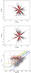 |
Fig. 1. Presentation of our sample. Upper and middle panels: location of the K2 sample considered in this work in galactocentric coordinates, (X, Y) and (X, Z) planes, respectively. The whole sample is in gray, and the young α-rich stars are represented with red dots. Lower panel: Hertzsprung–Russell diagram for stars in our sample, compared with stellar tracks from Miglio et al. (2021) with [m/H] = −0.25 and different masses (1 M⊙ in blue, 1.4 M⊙ in green, 1.8 M⊙ in orange). The high-α stars are in gray, and the young α-rich stars are represented with red dots. |
Our targets were also observed by the APOGEE and GALAH surveys. The chemical abundances used here are those given by the APOGEE Stellar Parameters and Chemical Abundances Pipeline (ASPCAP; García Pérez et al. 2016). A full description of this pipeline as applied to APOGEE DR17 is given in Holtzman et al. (in prep.). We discarded targets with ASPCAPFLAG having STAR_BAD or STAR_WARN, and with RV_FLAG. We complemented our analysis by using GALAH data for neutron-capture elements not available in APOGEE. Regarding GALAH, we considered the chemical abundances from GALAH DR3 (Buder et al. 2021). In this case, we considered only the elemental abundances with flag_X_fe==0 (see Buder et al. 2021) for the neutron-capture elements considered in this work.
We then used astrometric information from Gaia DR3 (Gaia Collaboration 2022). We discarded targets with ruwe> 1.4 or those marked as binaries by non_single_stars flag (Lindegren 2018).
2.2. Inferring stellar ages and orbital parameters
Masses, radii, ages, and distances are inferred by using the code PARAM (da Silva et al. 2006; Rodrigues et al. 2014, 2017), which makes use of a Bayesian inference method. PARAM takes as input a combination of asteroseismic indices and spectroscopic constraints, such as νmax, [Fe/H], [α/Fe], Teff, and either L or Δν.
To explore potential systematics, we inferred masses and ages using two sets of constraints. While Teff and metallicity are included in both cases, in one set we considered as constraints νmax and L, in the second set νmax and Δν. As shown in Tailo et al. (2022), among others, datasets of relatively short duration may be subject to systematics on the measurement of Δν; this is particularly relevant in the case of low-metallicity core-He-burning stars (see also Matteuzzi et al. 2023; Willett et al., in prep.). In the set of ages inferred including Δν, we removed targets when their mass inferred using (νmax, Δν) differs from that determined by (νmax, L) by more than 50%. Given the direct impact on the high-α population, in the following we explore and check the results and trends in both datasets.
Luminosities were computed using extinctions from the Bayestar19 dustmap (Green et al 2019) implemented in the dustmaps Python package (Green 2018) and bolometric corrections computed through the code by Casagrande & VandenBer (2014, 2018a,b). We used the luminosity derived from  +17 μas, L17. Distances were deduced from the Gaia parallax, whereas in the (νmax, Δν) sample they come from PARAM.
When using PARAM, we considered a lower limit of 0.05 dex for the uncertainty on [Fe/H] and of 50 K for the uncertainty on Teff, due to the very low (internal) uncertainties quoted in APOGEE DR17 (see also, Casali et al. 2023). The grid of stellar models used here is the reference one adopted in the work of Miglio et al. (2021), where a detailed explanation of the method can be found.
We then computed the orbital parameters by using the fast orbit estimation method of Mackereth & Bovy (2018), implemented in the GalPy package (Bovy 2015), where the Milky Way potential MWPotential2014 for the gravitational potential of the Milky Way is assumed (Bovy 2015). We assume that the radial position of the Sun is RGal, ⊙ = 8 kpc and the circular velocity vcirc = 220 km s−1 (Bovy et al. 2012), the Sun’s motion with respect to the local standard of rest [U, V, W]⊙ = [ − 11.1, 12.24, 7.25] km s−1 (Schönrich et al. 2010), and that the vertical offset of the Sun from the Galactic plane is ZGal, ⊙ = 20.8 pc (Bennett & Bovy 2019).
The final reference sample considered here consists of ∼6000 stars with available asteroseismic, spectroscopic, and astrometric information. For further details on the observational sample, we refer to the catalogue paper by Willett et al. (in prep.).
3. Are young α-rich stars similar to old high-α populations?
Here, we show the results for our sample of stars with available stellar ages from K2, chemical abundances from APOGEE and GALAH, and astrometric information from Gaia. We start by defining the young α-rich stars in our sample. Then, we discuss their chemical and kinematic properties. Our discussion is focused on APOGEE, and we use the GALAH data to complement our analysis with respect to neutron-capture elements.
3.1. Definition
First, we define the young α-rich stars in our K2-APOGEE sample, as was done in Chiappini et al. (2015), with the CoRoGEE sample on the basis of the [Mg/Fe] versus [Fe/H] plot (see Fig. 2). This is a well-known diagram to define young α-rich stars (see also more recently Sun et al. 2020; Zhang et al. 2021; Cerqui et al. 2023), but we now extend the asteroseismic study of Chiappini et al. (2015) by using our new K2 sample covering larger spatial baselines and with a much larger sample (ten times larger than the CoRoGEE sample).
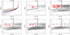 |
Fig. 2. [Mg/Fe] vs. age diagrams. Upper left panel: predictions of models of the thin disk at different radii: 4 kpc in gray, 6 kpc in purple, 8 kpc in blue, 10 kpc in green, 12 kpc in orange, 14 kpc in red (see Chiappini 2009; Grisoni et al. 2017, 2018). In the other panels the observational data are shown for our sample in different bins of guiding radius. The black lines in the various plots mark the “forbidden region” as defined in Chiappini et al. (2015). The red dots are the young α-rich stars selected in our sample. We report the 1σage error bars. |
In the upper left panel of Fig. 2, we show the region in the [Mg/Fe] versus age plot that cannot be explained by means of chemical evolution models of the Galactic thin disk at different galactocentric distances, as suggested in Chiappini et al. (2015). The chemical evolution model is a multi-zone model for the Galactic thin disk at different galactocentric distances (see Chiappini 2009, and consistently the recent results of Grisoni et al. 2017, 2018). We then define the young α-rich stars in our sample as being high-α stars ([Mg/Fe] > 0.2 dex) and with young ages, well-inside the forbidden region defined by models. Specifically, they should be inside the forbidden region and be at least 1σage away from the border of the selection region.
In the following sections, we compare the properties of our young α-rich stars to other populations, namely the old high-α stars (i.e., the high-α stars not defined as young α-rich) and the low-α stars. We divide our high- and low-α populations by considering a division in Mg, where the dichotomy is more evident (see, e.g., discussion in Grisoni et al. 2017). In particular, we consider [Mg/Fe] > 0.2 and [Mg/Fe] ≤ 0.2, respectively, for the high- and low-α sequences. We perform this separation at [Mg/Fe] corresponding to 0.2 dex in order to obtain a “genuine” high-α sequence (Miglio et al. 2021; Queiroz et al. 2023), not including the transition–bridge region in our high-α definition (Anders et al. 2018; Ciucă et al. 2021).
We report the results in Table 1 and associate an uncertainty on the fraction of young α-rich stars, by bootstrapping 1000 realizations of the data by taking into account uncertainties in age and calculating the deviation of the distribution of the number of young α-rich stars. We find that the fraction of young α-rich stars with respect to the high-α population is around 7–10% (see also Montalbán et al. 2021; Miglio et al. 2021).
Young α-rich stars in different Galactic regions.
We note that the final fraction of young α-rich stars can be affected by systematics. Comparing the (νmax, L) and (νmax, Δν) samples gives an estimate of potential systematics in the asteroseismic measurements. In particular, given our K2-APOGEE sample with all the required checks and flags, we also tested our second age dataset with ages from (νmax, Δν); in this case, we get a slightly higher fraction of young α-rich stars, but also in this case our main findings are not affected. We also tested other possible systematics in our definition of young α-rich stars for our reference sample. First, we varied the threshold in the definition (without the 1σage constraint or with a stricter 2σage constraint) and, in this case, the fraction of young α-rich stars can vary from ∼5 to 15%, but the spatial trends remain constant and are not affected by the definition. We note also that, in addition to the threshold on the forbidden region, the choice itself of the α-element considered might also affect the final results, but still within the range discussed above; as previously discussed, here we choose Mg where the dichotomy between the two sequences is very evident. We note that a very large sample is available, but when doing such analyses with more biased samples (see, e.g., Matsuno et al. 2018; Jofré et al. 2023) the selection of groups can be a limiting factor that should be considered. We also note that the fraction of young α-rich stars is higher in the red clump with respect to the red-giant branch, supporting the scenario in which most of these stars might have gone through interaction with a companion (see also Miglio et al. 2021).
In conclusion, even if the fraction of young α-rich stars found in our sample can be slightly affected by the above-mentioned systematics, the spatial trends across different parts of the Galaxy that we recover and discuss in detail in the next sections are still preserved.
3.2. Spatial properties
Once our sample of young α-rich stars has been defined, we study its spatial distribution in the Galaxy. In the various panels of Fig. 2, we show the observational results for our K2-APOGEE sample at different bins of guiding radius Rg (the radius of a circular orbit of the same angular momentum). In particular, we use the following bins of Rg (see also Casali et al. 2023): Rg < 5 kpc, 5–7 kpc, 7–8 kpc, 8–10 kpc, Rg > 10 kpc. We make use of guiding radius rather than galactocentric distance to mitigate blurring (see also Willett et al. 2023, and references therein).
From the various panels of Fig. 2, it is clear that similar fractions of young α-rich stars are present in different parts of the Galaxy, from the innermost Galactic regions to the outer ones. As found in Chiappini et al. (2015) and Martig et al. (2015), the fraction of young α-rich stars with respect to the total number of stars is higher in the innermost part of the Galaxy, where the high-α sequence is dominating (see, e.g., Table 1 in Chiappini et al. 2015). However, at variance with Chiappini et al. (2015) where young α-rich stars seemed more abundant toward the inner Galactic disk regions, and therefore suggested the origin of these stars to be related to the complex chemical evolution that takes place near the co-rotation region of the Galactic bar, we find a significant number of young α-rich stars also in other bins of distance, where the high-α sequence extends. In particular, it is important to look at the fraction of young α-rich stars with respect to the number of high-α stars, which remains almost constant across the Galaxy. With both our age samples, we find that the fraction of young α-rich stars with respect to the total decreases going outward in guiding radius, whereas the fraction with respect to the number of high-α stars remains almost constant within the errors in the different bins.
To summarize, in our sample the young α-rich stars appear in different Galactic locations, where the high-α sequence extends (Hayden et al. 2015; Queiroz et al. 2020). Therefore, this supports the idea that they can be part of the high-α population: they should have formed from the same gas as the high-α sequence, but they might be affected by binary evolution (Izzard et al. 2018).
Similarly, we investigate our results for the whole sample in three different bins in Galactic height (|Z|< 0.5, between 0.5–1 kpc, and > 1 kpc). The results concerning the number of young α-rich found in these bins are summarized directly in Table 1. We can see in this case that the number of young α-rich stars with respect to the total increases with height, as is expected since the high-α sequence becomes dominant with respect to the low-α when going to greater height away from the Galactic plane (Hayden et al. 2015; Queiroz et al. 2020). Still, the number of young α-rich stars with respect to the high-α population remains almost constant, in agreement with what has been found as a function of guiding radius. Thus, the occurrence of young α-rich stars does not depend on the location in the Galaxy, at variance with what was suggested by Chiappini et al. (2015) with CoRoGEE. This is found thanks to a much larger sample of stars in different parts of the Galaxy, which extends the previous results found in the literature.
3.3. Chemical properties
After showing the [Mg/Fe] versus age plots used to define our sample of young α-rich stars and investigate their occurrence rate in different parts of the Galaxy, we further investigate the chemical properties of our sample of young α-rich stars by also looking at other chemical abundance patterns of different chemical elements considered reliable in APOGEE DR17 release (Abdurro’uf et al. 2022), and we use the GALAH DR3 data (Buder et al. 2021) to complement our analysis with respect to neutron-capture elements.
3.3.1. Metallicity
We investigate the dependence on metallicity (i.e., [Fe/H]), by looking at different bins in [Fe/H] for our K2-APOGEE sample. The results of the various [Fe/H] bins are then directly reported in Table 2.
Young α-rich stars (YAR) in different bins of metallicity.
We find that young α-rich stars are more dominant in metal-poor regimes, where the high-α sequence is dominating with respect to the total number of stars. With respect to the number of high-α stars, we still find a fraction of ∼7–10% for the young α-rich stars, although with a slightly increasing trend with decreasing metallicity at the uncertainty level in the (νmax, Δν) sample; this tentative trend is not there in the (νmax, L) sample. We note that there is evidence for an increased intrinsic fraction of close binaries in metal-poor regimes (see El-Badry & Rix 2019; Moe et al. 2019) and an increased fraction of blue stragglers among old metal-poor stars (Fuhrmann et al. 2017; Casagrande 2020), with a more evident trend with decreasing metallicity with respect to what we find. Part of the difference could be that we likely removed (some) binary stars from our sample, due to our selection criteria (e.g., ruwe).
In addition, we find the fraction of our young α-rich stars in the field to be similar to that of overmassive red giant stars found recently in open clusters, where they estimate an occurrence rate of around 10% and 5–10% in the old-open clusters NGC6819 and NGC6791 (Brogaard et al. 2016, 2021; Handberg et al. 2017), indicating that about 10% of the red giants in the cluster have experienced mass transfer or a merger. These facts suggest that ∼10% of the low-α field stars could also have their ages underestimated by asteroseismology. This should be kept in mind when using asteroseismic ages to interpret results in Galactic archaeology.
3.3.2. α-elements
Recently, Jofré et al. (2023) and Cerqui et al. (2023) also studied the nature of young α-rich stars in the light of APOGEE data, but here we present new results based on stellar ages coming from asteroseismology, and thus providing a complementary analysis with respect to the above-mentioned works. In Fig. 3 we show our [X/Fe] versus [Fe/H] plots for the different chemical elements considered reliable in APOGEE DR17.
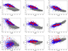 |
Fig. 3. [X/Fe] vs. [Fe/H] plots for various chemical elements in our K2-APOGEE sample. The red dots represent the young α-rich stars, blue dots the old high-α stars, and gray dots the low-α stars. |
We investigate the abundance patterns of the three populations introduced and defined at the beginning of Sect. 3: young α-rich stars (in red), old high-α stars (in blue), and low-α stars (as background in gray). After performing the separation among the three populations in the [Mg/Fe], we also investigate the various [X/Fe] versus [Fe/H] diagrams for other chemical elements available and considered reliable in APOGEE DR17. We can see that, in general, the distribution of young α-rich stars resembles that of high-α stars rather than the low-α distribution, in agreement with previous studies. Thus, the young α-rich stars have chemical properties that are more similar to the high-α population, in agreement with previous abundance analyses where they indeed show that the majority of the young α-rich stars have chemical abundances similar to the high-α stars rather than the low-α stars at similar ages. Consistent results have been seen, for example, in Matsuno et al. (2018) using high-resolution spectroscopic follow-up, and more recently in Jofré et al. (2023) and Cerqui et al. (2023) also using chemical abundances from APOGEE, but very different ages with respect to our asteroseismic estimates that can provide a complementary support to the idea that young α-rich stars should be considered stragglers of the thick disk, at variance with alternative scenarios present in the literature.
In the following, to be more quantitative, we look at the corresponding histograms for the various [X/Fe] abundance ratios considered, similarly to what was done by Zhang et al. (2023) with LAMOST data, but here for our APOGEE and GALAH data. In Fig. 4, we show the corresponding histograms for the different chemical elements color-coded according to the different populations investigated in this work. In the case of Mg, the dichotomy between high- and low-α stars is evident (see, e.g., Grisoni et al. 2017), and we chose this chemical element to perform the separation between the high- and low-α populations. For Mg, the young α-rich stars are then part of the high-α population, by definition.
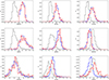 |
Fig. 4. [X/Fe] vs. [Fe/H] plots for various chemical elements in our K2-APOGEE sample for the young α-rich stars (in red), old high-α stars (in blue), and the low-α stars (in gray). |
Then, we look at the other α-elements, whether the separation is still evident and the young α-rich stars follow the chemistry of the old high-α sequence. Also in the case of the other α-elements considered here, we can see that in general the high- and low-α populations can be well separated, and the young α-rich stars share the same locus of the high-α population in the different diagrams.
3.3.3. Aluminum
Aluminum is an odd-Z element. From Fig. 4 we can see that also in this case the histogram clearly shows a bimodal distribution, and that the young α-rich stars closely follow the high-α population.
3.3.4. Manganese
Manganese is a Fe-peak element. In this case the bimodality is not as clear, and high-α and low-α stars are not clearly separated. Even so, the young α-rich stars show a distribution in agreement with the high-α population.
3.3.5. Cerium
Cerium is the only s-process element available in APOGEE DR17 (see Casali et al. 2023, for a detailed study of the Ce abundances for our K2-APOGEE sample). In the case of Ce, the differences between the various populations are expected to be smaller, as predicted by chemical evolution models (see, e.g., Grisoni et al. 2020). In the [Ce/Fe] versus [Fe/H] plot (see Fig. 3), there is a large spread, and it is difficult to draw firm conclusions whether young α-rich stars are Ce-enhanced with respect the rest of the high-α sequence. In the histogram of Ce (see Fig. 4), the dichotomy between the various populations is not evident: the various populations are mixed and it is more difficult to disentangle them. For example, Grisoni et al. (2020) showed that the thick and thin disk populations are mixed in the abundance patterns of s-process elements such as Ce (see also Contursi et al. 2023), and it is more difficult to disentangle them at variance with α-elements, where the dichotomy between the two populations is evident. Since Ce is the only neutron-capture element available in APOGEE DR17 and it is difficult to draw firm conclusions, we decided to complement our analysis by performing a cross-match with GALAH DR3 in order to look at other neutron-capture elements.
3.3.6. Other s-process elements with GALAH
To better investigate neutron-capture elements, we took advantage of our K2-APOGEE sample cross-matched with GALAH DR3: in particular, we now consider the stars in our K2 sample that are in common between APOGEE and GALAH, where other s-process elements are available. For consistency, we mantain the same definition of young α-rich stars as for the reference K2-APOGEE sample and complement it with information from GALAH. We now have a subsample of ∼2500 stars, with the available abundances of neutron-capture elements from GALAH.
In particular, we show results for Y, Ba, and La. Even if the scatter is higher with respect to APOGEE, this allows us to complement the analysis for neutron-capture elements not available in APOGEE.
From Fig. 5 we can see a mild s-process enhancement, but it is still difficult to clearly assess whether there is a clear difference in s-process enhancement between the two populations (young α-rich stars and old high-α stars). Therefore, further data on s-process elements are needed to establish whether the young α-rich stars have peculiar properties regarding the abundance of s-process elements. Looking at the abundance patterns of s-process elements can be important since they can also point toward some accretion of material. Zhang et al. (2021) took advantage of data from the LAMOST survey and found that the young α-rich stars were significantly Ba-enhanced compared to most of the high-α old stars. They explained the observed Ba-enhancement of the young α-rich stars with the scenario that the stars are formed via binary evolution and, in particular, that they might have accreted Ba-rich materials from their AGB companions (Bidelman & Keenan 1951; Jorissen et al. 2019; Escorza et al. 2019; Zhang et al. 2023). Such Ba enhancement of these young α-rich stars was different from the findings of Yong et al. (2016) and Matsuno et al. (2018) who showed that the [Ba/Fe] ratios of the young α-rich stars seem to be comparable to those of the old high-α stars. In the works of Yong et al. (2016) and Matsuno et al. (2018) it was found that Ba and other s-process elements were not systematically enhanced in young α-rich stars and the reason might be related to the nature of the mass transfer (happening before the primary reaches the AGB; Izzard et al. 2018; Jofré et al. 2023). Our results seem to confirm the Matsuno et al. (2018) results with a larger sample, but further data might be needed to draw firm conclusions in this context.
3.3.7. C and N
Other chemical elements that can give very important hints about stellar evolution processes are C and N (Romano 2022 for a detailed review). From Fig. 3 and more evidently from the histograms in Fig. 4, we can see that for these elements there are clear differences between the old high-α and the young α-rich stars, especially for N. We recall that the surface abundances of C and N are affected by the first dredge-up, with higher mass stars dredging up material with increased He and N and decreased C and Li (Salaris et al. 2015, 2018). The changes in C and N are thus a result of the burning in the interior, which is dominated by the CNO cycle. The offset in C and N for some of the young α-rich stars most probably arises from the higher masses of the young α-rich population (see also Hekker & Johnson 2019). From our data we can also see that young α-rich stars seem to present slightly lower C abundances and more evidently higher N abundances with respect to the old high-α stars. We note the presence of many N-rich stars in our sample (see also Schiavon et al. 2017; Fernández-Trincado et al. 2022).
Differences in C and N are then reflected in the [C/N] ratio itself. Further insights into the nature of the young α-rich stars stars can thus be gained from the [C/N] ratio (see, e.g., Hekker & Johnson 2019; Jofré et al. 2016, 2023; Izzard et al. 2018; Sun et al. 2020; Miglio et al. 2021; Cerqui et al. 2023). In Fig. 6 we focus on the [C/N] ratios of the stars in our sample. As can be seen from the histogram (left panel), the young α-rich stars (red line) lie closer to the low-α (gray line), differing substantially from the distribution of the old high-α stars (blue line). Since part of this difference is expected, due to the higher masses of the young α-rich stars compared to old high-α stars, at least one more dimension is needed to identify potential signs of binary evolution. Therefore, in the other two panels in the figure we show the [C/N] ratio as a function of mass. In the middle panel the three samples are shown (low-α, high-α stars, young α-rich, color-coded as in the left panel). We also overplot three curves representing stellar model predictions from Vincenzo et al. (2021) of the dependency of the [C/N] ratio with stellar mass. The purpose is to illustrate what we state above (i.e., that lower ratios are expected for higher masses). However, the curves are not meant to fit the data as here there is a complex mix of stellar populations (see, e.g., discussion in Anders et al. 2018), and thus it is beyond of the scope of the present work to identify debris from past accretion, debris from globular clusters, or stars migrating from their original birth radii. Focusing on the stellar evolution aspects alone, we see a larger spread in the [C/N] ratio at a given mass for the young α-rich stars (red) with respect to what is seen in the low-α sample (gray). The young α-rich stars with [C/N] values above the general trend can arise if the current star is the result of a merger or mass transfer between two lower-mass giants that have preserved their original [C/N] values. A more detailed explanation is given in Jofré et al. (2016); their Fig. 5 shows a simulation of [C/N] versus age for a stellar population including binary evolution. The simulation predicts that many of the interacting binaries result in a sequence of stars where [C/N] does not depend on mass and remains high independently of the mass. Though we have relatively few such stars, we do see a number of stars that scatter close to the [C/N] = 0 line above the general single-star trend, which are consistent with this scenario. Importantly, these conclusions remain valid even if one considers shifting the single-star theoretical predictions in the middle panel of Fig. 6 upward to follow the upper envelope of the observed low-α star sequence. Some of the α-rich stars show very high [C/N] ratios. These large ratios are also seen in some of the high-α sample (blue). In the right panel, where we color-code our samples according to metallicity, it can be seen that most of the stars with very high [C/N] ratios tend to be more metal-poor (C-enhanced stars). The high [C/N] values for the young α-rich stars can thus also be a hint of binary mergers or mass accretion, in this case for stars that started out with higher abundances of C.
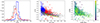 |
Fig. 6. [C/N] ratio. Left panel: histogram for [C/N] of the stars in our K2 sample (gray, blue, and red histograms represent the low-α, old high-α, and young α-rich samples, respectively). Middle panel: [C/N] vs. mass for the stars in our sample, with colors as in the left panel. The solid lines represent the predictions of stellar evolution models from Vincenzo et al. (2021) at different metallicities ([Fe/H] = −1 in yellow, −0.5 in green, and +0.25 in purple). Right panel: [C/N] ratios for the entire sample color-coded by [Fe/H] (as indicated in the color scale). In this panel are shown low-α (dots), old high-α (triangles), and young-α rich stars (bigger dots). |
Further observational evidence would be important to clearly assess the nature of these stars, but to the best of our knowledge there is currently no other explanation for the [C/N] values being higher than the single-star trend, while they are consistent with the simulations in the case of binary mergers or mass transfer.
3.4. Kinematic properties
In this section, we look at the kinematics of these young α-rich stars and address the question of whether the old high-α and the young α-rich stars differ in kinematics. In Fig. 7 we show the distribution of guiding radius Rg, Zmax, and eccentricity for the three different populations (young α-rich, old high-α, and low-α). From this figure we can see that the young α-rich stars share similar properties with the old high-α population: they are vertically hotter than the low-α population and they display properties in agreement with the distribution of the rest of the old high-α sequence in Rg, Zmax, and eccentricity. This seems to be inconsistent with previous interpretations of the spatial distribution of these young α-rich stars as coming from the inner part of the Galaxy (Chiappini et al. 2015), suggesting that they formed in the bar region and migrated outward. This scenario could be the result of an incomplete sampling in previous studies. Conversely, as found by many other studies (Martig et al. 2015; Silva Aguirre et al. 2018), we can see that the kinematics of our young α-rich stars is more similar to old high-α stars rather than the low-α stars with similarly young ages. These findings support the scenario in which the majority of these young α-rich stars share the same properties of the genuine high-α population, and thus the idea that they are part of the high-α sequence, but they are probably products of mergers or mass accretion from a companion star (Martig et al. 2015; Yong et al. 2016; Jofré et al. 2016, 2023; Zhang et al. 2021; Miglio et al. 2021). Consistent trends were found by Sun et al. (2020) and were also discussed in Jofré et al. (2023) and Cerqui et al. (2023). They all conclude that young α-rich stars should be considered stragglers of the thick disk, at variance with alternative scenarios proposed in the literature. Our results can thus complement and support these conclusions with a new sample accounting for precise ages coming from asteroseismology.
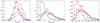 |
Fig. 7. Distribution function of guiding radii Rg (left panel), Zmax (middle panel), and eccentricity (right panel) for the different populations considered: young α-rich (in red), old high-α (blue), low-α (gray). |
To summarize, with our new K2 sample we are able to study young α-rich stars in different parts across the Galaxy and investigate in detail their spatial distribution, chemical properties, and kinematic properties. We find that these stars are present in every bin of galactocentric distance and Galactic heights, where the high-α sequence is present. They present chemical and kinematic properties that are more similar to the high-α stars than the low-α stars at the same age. Therefore, these young α-rich stars are like high-α, but might be the product of binary evolution with merger or accretion, in agreement with previous studies (Yong et al. 2016; Jofré et al. 2016, 2023; Zhang et al. 2021) rather than related to a peculiar chemical evolution scenario near the co-rotation region (Chiappini et al. 2015).
4. Summary and conclusions
In this paper, we investigated the nature of young α-rich stars in an unprecedented sample of ∼6000 red giants observed with K2, with spectroscopic information from APOGEE DR17 and GALAH DR3, then cross-matched with Gaia. Our new K2 sample spans a wider range of locations in the Galaxy, and thus allowed us to perform a novel more comprehensive analysis of young α-rich stars in the Galaxy with respect to previous asteroseismic studies in the literature, such as that of Chiappini et al. (2015) with CoRoGEE. Moreover, with its precise asteroseismic ages, it allowed us to complement other recent studies of young α-rich stars (see, e.g., Jofré et al. 2023; Cerqui et al. 2023), whose nature is still very much debated in Galactic archaeology.
Our main conclusions are as follows:
-
By applying the definition of young α-rich stars in the [Mg/Fe] versus age plot, we define our sample of young α-rich stars. We find that the fraction of young α-rich stars with respect to the high-α population is around 7–10% (see also Montalbán et al. 2021; Miglio et al. 2021), and we discuss possible systematics affecting this fraction.
-
The young α-rich stars present in our sample are found in each bin of Rg (from less than 4.5 kpc to above 10.5 kpc). The percentage of young α-rich stars with respect to the total number of stars decreases with guiding radius since the high-α sequence becomes less dominant; however, the percentage of young α-rich stars with respect to the number of high-α stars remains constant.
-
Similarly, we investigated the presence of young α-rich stars in different bins of |Z| and found that they become more dominant at higher |Z| since the high-α sequence becomes more dominant; even so, the fraction of young α-rich stars with respect to the high-α population stays constant (∼7–10% ). Thus, independently of the definition, we highlight the fact that the fraction of young α-rich stars with respect to the number of high-α stars remains almost constant across different parts of the Galaxy.
-
If the young α-rich stars are interpreted as having gained mass through binary evolution, our findings are also in agreement with studies of open clusters where an occurrence rate of overmassive red giant stars of about 10% has also been found (Handberg et al. 2017; Brogaard et al. 2018, 2021).
-
Concerning the chemical properties, we considered APOGEE DR17 chemical abundances and found that young α-rich stars share similar chemical abundances to those of the old high-α population, except for elements such as C and N.
-
We also used GALAH DR3 chemical abundances to complement our analysis with respect to neutron-capture elements not available in APOGEE. In particular, we considered Y, Ba, and La, and found a mild s-process enhancement. Even so, it was not possible to assess whether there are clear differences in s-process elements between young α-rich stars and the old high-α ones, and new data of higher precision would be valuable.
-
We also found that the kinematic properties of young α-rich stars in our sample look similar to those of the high-α sequence rather than the low-α sequence.
With our new K2 sample that spans a wider range of galactocentric distances than before, we conclude that young α-rich stars are present in different parts of the Galaxy and that they share the same properties as the normal α-rich population, except for [C/N]. Binary evolution with accretion and/or mergers are naturally consistent with these findings.
Acknowledgments
We thank the referee for useful comments and suggestions that improved our paper. V.G., C.C., A.M., K.B., G.C., E.W., J.M., A.S., J.S.T., M.T., M.M. acknowledge support from the ERC Consolidator Grant funding scheme (project ASTEROCHRONOMETRY, https://www.asterochronometry.eu, G.A. n. 772293). V.G. and C.C. acknowledge support from the EU COST Action CA16117 (ChETEC). C.C. acknowleges Fundación Jesús Serra for its great support during her visit to IAC, Spain, during which part of this work was written. Funding for the Stellar Astrophysics Centre is provided by The Danish National Research Foundation (Grant agreement No. DNRF106). Y.E. acknowledges support from the School of Physics and Astronomy, University of Birmingham. V.G. also acknowledges financial support from INAF under the program “Giovani Astrofisiche ed Astrofisici di Eccellenza – IAF: Astrophysics Fellowships in Italy” (Project: GalacticA, “Galactic Archaeology: reconstructing the history of the Galaxy”).
References
- Abdurro’uf, Accetta, K., Aerts, C., et al. 2022, ApJS, 259, 35 [NASA ADS] [CrossRef] [Google Scholar]
- Anders, F., Chiappini, C., Santiago, B. X., et al. 2014, A&A, 564, A115 [NASA ADS] [CrossRef] [EDP Sciences] [Google Scholar]
- Anders, F., Chiappini, C., Rodrigues, T. S., et al. 2017, A&A, 597, A30 [NASA ADS] [CrossRef] [EDP Sciences] [Google Scholar]
- Anders, F., Chiappini, C., Santiago, B. X., et al. 2018, A&A, 619, A125 [NASA ADS] [CrossRef] [EDP Sciences] [Google Scholar]
- Baglin, A., Auvergne, M., Boisnard, L., et al. 2006, in 36th COSPAR Scientific Assembly, 36, 3749 [Google Scholar]
- Bennett, M., & Bovy, J. 2019, MNRAS, 482, 1417 [NASA ADS] [CrossRef] [Google Scholar]
- Bensby, T., Feltzing, S., & Oey, M. S. 2014, A&A, 562, A71 [NASA ADS] [CrossRef] [EDP Sciences] [Google Scholar]
- Bergemann, M., Ruchti, G. R., Serenelli, A., et al. 2014, A&A, 565, A89 [NASA ADS] [CrossRef] [EDP Sciences] [Google Scholar]
- Bidelman, W. P., & Keenan, P. C. 1951, ApJ, 114, 473 [Google Scholar]
- Borisov, S., Prantzos, N., & Charbonnel, C. 2022, A&A, 668, A181 [NASA ADS] [CrossRef] [EDP Sciences] [Google Scholar]
- Bovy, J. 2015, ApJS, 216, 29 [NASA ADS] [CrossRef] [Google Scholar]
- Bovy, J., Allende Prieto, C., Beers, T. C., et al. 2012, ApJ, 759, 131 [NASA ADS] [CrossRef] [Google Scholar]
- Brogaard, K., Jessen-Hansen, J., Handberg, R., et al. 2016, Astron. Nachr., 337, 793 [NASA ADS] [CrossRef] [Google Scholar]
- Brogaard, K., Christiansen, S. M., Grundahl, F., et al. 2018, MNRAS, 481, 5062 [Google Scholar]
- Brogaard, K., Arentoft, T., Jessen-Hansen, J., & Miglio, A. 2021, MNRAS, 507, 496 [NASA ADS] [CrossRef] [Google Scholar]
- Buck, T. 2020, MNRAS, 491, 5435 [NASA ADS] [CrossRef] [Google Scholar]
- Buder, S., Sharma, S., Kos, J., et al. 2021, MNRAS, 506, 150 [NASA ADS] [CrossRef] [Google Scholar]
- Casagrande, L. 2020, ApJ, 896, 26 [NASA ADS] [CrossRef] [Google Scholar]
- Casagrande, L., & VandenBerg, D. A. 2014, MNRAS, 444, 392 [Google Scholar]
- Casagrande, L., & VandenBerg, D. A. 2018a, MNRAS, 479, L102 [NASA ADS] [CrossRef] [Google Scholar]
- Casagrande, L., & VandenBerg, D. A. 2018b, MNRAS, 475, 5023 [Google Scholar]
- Casagrande, L., Silva Aguirre, V., Schlesinger, K. J., et al. 2016, MNRAS, 455, 987 [Google Scholar]
- Casali, G., Grisoni, V., Miglio, A., et al. 2023, A&A, 677, A60 [NASA ADS] [CrossRef] [EDP Sciences] [Google Scholar]
- Cerqui, V., Haywood, M., Di Matteo, P., Katz, D., & Royer, F. 2023, A&A, 676, A108 [NASA ADS] [CrossRef] [EDP Sciences] [Google Scholar]
- Chiappini, C. 2009, in The Galaxy Disk in Cosmological Context, eds. J. Andersen, B. M. Nordströara, & J. Bland-Hawthorn, 254, 191 [Google Scholar]
- Chiappini, C., Matteucci, F., & Gratton, R. 1997, ApJ, 477, 765 [Google Scholar]
- Chiappini, C., Anders, F., Rodrigues, T. S., et al. 2015, A&A, 576, L12 [NASA ADS] [CrossRef] [EDP Sciences] [Google Scholar]
- Ciucă, I., Kawata, D., Miglio, A., Davies, G. R., & Grand, R. J. J. 2021, MNRAS, 503, 2814 [Google Scholar]
- Contursi, G., de Laverny, P., Recio-Blanco, A., et al. 2023, A&A, 670, A106 [NASA ADS] [CrossRef] [EDP Sciences] [Google Scholar]
- Cui, X.-Q., Zhao, Y.-H., Chu, Y.-Q., et al. 2012, Res. Astron. Astrophys., 12, 1197 [Google Scholar]
- da Silva, L., Girardi, L., Pasquini, L., et al. 2006, A&A, 458, 609 [NASA ADS] [CrossRef] [EDP Sciences] [Google Scholar]
- De Silva, G. M., Freeman, K. C., Bland-Hawthorn, J., et al. 2015, MNRAS, 449, 2604 [NASA ADS] [CrossRef] [Google Scholar]
- El-Badry, K., & Rix, H.-W. 2019, MNRAS, 482, L139 [NASA ADS] [Google Scholar]
- Elsworth, Y., Themeßl, N., Hekker, S., & Chaplin, W. 2020, Res. Notes Am. Astron. Soc., 4, 177 [Google Scholar]
- Escorza, A., Karinkuzhi, D., Jorissen, A., et al. 2019, A&A, 626, A128 [NASA ADS] [CrossRef] [EDP Sciences] [Google Scholar]
- Fernández-Trincado, J. G., Beers, T. C., Barbuy, B., et al. 2022, A&A, 663, A126 [NASA ADS] [CrossRef] [EDP Sciences] [Google Scholar]
- Fuhrmann, K. 1998, A&A, 338, 161 [NASA ADS] [Google Scholar]
- Fuhrmann, K., Chini, R., Kaderhandt, L., & Chen, Z. 2017, ApJ, 836, 139 [Google Scholar]
- Gaia Collaboration (Prusti, T., et al.) 2016, A&A, 595, A1 [NASA ADS] [CrossRef] [EDP Sciences] [Google Scholar]
- Gaia Collaboration (Vallenari, A., et al.) 2023, A&A, 674, A1 [NASA ADS] [CrossRef] [EDP Sciences] [Google Scholar]
- García Pérez, A. E., Allende Prieto, C., Holtzman, J. A., et al. 2016, AJ, 151, 144 [Google Scholar]
- Gilliland, R. L., Brown, T. M., Christensen-Dalsgaard, J., et al. 2010, PASP, 122, 131 [Google Scholar]
- Gilmore, G., Randich, S., Asplund, M., et al. 2012, The Messenger, 147, 25 [NASA ADS] [Google Scholar]
- Green, G. M. 2018, J. Open Source Software, 3, 695 [NASA ADS] [CrossRef] [Google Scholar]
- Green, G. M., Schlafly, E., Zucker, C., Speagle, J. S., & Finkbeiner, D. 2019, ApJ, 887, 27 [Google Scholar]
- Grisoni, V., Spitoni, E., Matteucci, F., et al. 2017, MNRAS, 472, 3637 [Google Scholar]
- Grisoni, V., Spitoni, E., & Matteucci, F. 2018, MNRAS, 481, 2570 [NASA ADS] [Google Scholar]
- Grisoni, V., Cescutti, G., Matteucci, F., et al. 2020, MNRAS, 492, 2828 [Google Scholar]
- Grisoni, V., Matteucci, F., & Romano, D. 2021, MNRAS, 508, 719 [NASA ADS] [CrossRef] [Google Scholar]
- Handberg, R., Brogaard, K., Miglio, A., et al. 2017, MNRAS, 472, 979 [CrossRef] [Google Scholar]
- Hayden, M. R., Bovy, J., Holtzman, J. A., et al. 2015, ApJ, 808, 132 [Google Scholar]
- Haywood, M., Di Matteo, P., Lehnert, M. D., Katz, D., & Gómez, A. 2013, A&A, 560, A109 [NASA ADS] [CrossRef] [EDP Sciences] [Google Scholar]
- Hekker, S., & Johnson, J. A. 2019, MNRAS, 487, 4343 [NASA ADS] [CrossRef] [Google Scholar]
- Howell, S. B., Sobeck, C., Haas, M., et al. 2014, PASP, 126, 398 [Google Scholar]
- Izzard, R. G., Preece, H., Jofre, P., et al. 2018, MNRAS, 473, 2984 [NASA ADS] [CrossRef] [Google Scholar]
- Jofré, P., Jorissen, A., Van Eck, S., et al. 2016, A&A, 595, A60 [Google Scholar]
- Jofré, P., Jorissen, A., Aguilera-Gómez, C., et al. 2023, A&A, 671, A21 [NASA ADS] [CrossRef] [EDP Sciences] [Google Scholar]
- Johnson, J. W., & Weinberg, D. H. 2020, MNRAS, 498, 1364 [CrossRef] [Google Scholar]
- Johnson, J. W., Weinberg, D. H., Vincenzo, F., et al. 2021, MNRAS, 508, 4484 [NASA ADS] [CrossRef] [Google Scholar]
- Jorissen, A., Boffin, H. M. J., Karinkuzhi, D., et al. 2019, A&A, 626, A127 [NASA ADS] [CrossRef] [EDP Sciences] [Google Scholar]
- Khoperskov, S., Haywood, M., Snaith, O., et al. 2021, MNRAS, 501, 5176 [NASA ADS] [CrossRef] [Google Scholar]
- Lindegren, L. 2018, Re-normalising the astrometric chi-square in Gaia DR2, Tech. Rep. [Google Scholar]
- Mackereth, J. T., & Bovy, J. 2018, PASP, 130, 114501 [Google Scholar]
- Mackereth, J. T., Miglio, A., Elsworth, Y., et al. 2021, MNRAS, 502, 1947 [NASA ADS] [CrossRef] [Google Scholar]
- Majewski, S. R., Schiavon, R. P., Frinchaboy, P. M., et al. 2017, AJ, 154, 94 [NASA ADS] [CrossRef] [Google Scholar]
- Martig, M., Rix, H.-W., Silva Aguirre, V., et al. 2015, MNRAS, 451, 2230 [NASA ADS] [CrossRef] [Google Scholar]
- Matsuno, T., Yong, D., Aoki, W., & Ishigaki, M. N. 2018, ApJ, 860, 49 [NASA ADS] [CrossRef] [Google Scholar]
- Matteucci, F. 2001, The Chemical Evolution of the Galaxy (Dordrecht: Kluwer Academic Publishers), 253 [Google Scholar]
- Matteucci, F. 2012, Chemical Evolution of Galaxies (Berlin, Heidelberg: Springer-Verlag) [Google Scholar]
- Matteucci, F. 2021, A&A Rev., 29, 5 [NASA ADS] [CrossRef] [Google Scholar]
- Matteuzzi, M., Montalbán, J., Miglio, A., et al. 2023, A&A, 671, A53 [NASA ADS] [CrossRef] [EDP Sciences] [Google Scholar]
- Miglio, A., Montalbán, J., Baudin, F., et al. 2009, A&A, 503, L21 [CrossRef] [EDP Sciences] [Google Scholar]
- Miglio, A., Chiappini, C., Morel, T., et al. 2013, MNRAS, 429, 423 [Google Scholar]
- Miglio, A., Chiappini, C., Mackereth, J. T., et al. 2021, A&A, 645, A85 [NASA ADS] [CrossRef] [EDP Sciences] [Google Scholar]
- Mikolaitis, Š., Hill, V., Recio-Blanco, A., et al. 2014, A&A, 572, A33 [NASA ADS] [CrossRef] [EDP Sciences] [Google Scholar]
- Mikolaitis, Š., de Laverny, P., Recio-Blanco, A., et al. 2017, A&A, 600, A22 [NASA ADS] [CrossRef] [EDP Sciences] [Google Scholar]
- Moe, M., Kratter, K. M., & Badenes, C. 2019, ApJ, 875, 61 [NASA ADS] [CrossRef] [Google Scholar]
- Montalbán, J., Mackereth, J. T., Miglio, A., et al. 2021, Nat. Astron., 5, 640 [Google Scholar]
- Pinsonneault, M. H., Elsworth, Y. P., Tayar, J., et al. 2018, ApJS, 239, 32 [Google Scholar]
- Queiroz, A. B. A., Anders, F., Chiappini, C., et al. 2020, A&A, 638, A76 [NASA ADS] [CrossRef] [EDP Sciences] [Google Scholar]
- Queiroz, A. B. A., Anders, F., Chiappini, C., et al. 2023, A&A, 673, A155 [NASA ADS] [CrossRef] [EDP Sciences] [Google Scholar]
- Recio-Blanco, A., de Laverny, P., Kordopatis, G., et al. 2014, A&A, 567, A5 [NASA ADS] [CrossRef] [EDP Sciences] [Google Scholar]
- Recio-Blanco, A., de Laverny, P., Palicio, P. A., et al. 2022, A&A, 674, A29 [Google Scholar]
- Rendle, B. M., Miglio, A., Chiappini, C., et al. 2019, MNRAS, 490, 4465 [NASA ADS] [CrossRef] [Google Scholar]
- Ricker, G. R., Winn, J. N., Vanderspek, R., et al. 2014, in Space Telescopes and Instrumentation 2014: Optical, Infrared, and Millimeter Wave, eds. J. Oschmann, M. Jacobus, M. Clampin, G. G. Fazio, & H. A. MacEwen, SPIE Conf. Ser., 9143, 914320 [Google Scholar]
- Rodrigues, T. S., Girardi, L., Miglio, A., et al. 2014, MNRAS, 445, 2758 [Google Scholar]
- Rodrigues, T. S., Bossini, D., Miglio, A., et al. 2017, MNRAS, 467, 1433 [NASA ADS] [Google Scholar]
- Rojas-Arriagada, A., Recio-Blanco, A., de Laverny, P., et al. 2017, A&A, 601, A140 [NASA ADS] [CrossRef] [EDP Sciences] [Google Scholar]
- Romano, D. 2022, A&A Rev., 30, 7 [NASA ADS] [CrossRef] [Google Scholar]
- Salaris, M., Pietrinferni, A., Piersimoni, A. M., & Cassisi, S. 2015, A&A, 583, A87 [NASA ADS] [CrossRef] [EDP Sciences] [Google Scholar]
- Salaris, M., Cassisi, S., Schiavon, R. P., & Pietrinferni, A. 2018, A&A, 612, A68 [NASA ADS] [CrossRef] [EDP Sciences] [Google Scholar]
- Schiavon, R. P., Johnson, J. A., Frinchaboy, P. M., et al. 2017, MNRAS, 466, 1010 [NASA ADS] [CrossRef] [Google Scholar]
- Schönrich, R., Binney, J., & Dehnen, W. 2010, MNRAS, 403, 1829 [NASA ADS] [CrossRef] [Google Scholar]
- Silva Aguirre, V., Bojsen-Hansen, M., Slumstrup, D., et al. 2018, MNRAS, 475, 5487 [NASA ADS] [Google Scholar]
- Spitoni, E., Silva Aguirre, V., Matteucci, F., Calura, F., & Grisoni, V. 2019, A&A, 623, A60 [NASA ADS] [CrossRef] [EDP Sciences] [Google Scholar]
- Spitoni, E., Verma, K., Silva Aguirre, V., et al. 2021, A&A, 647, A73 [EDP Sciences] [Google Scholar]
- Steinmetz, M., Zwitter, T., Siebert, A., et al. 2006, AJ, 132, 1645 [Google Scholar]
- Stello, D., Saunders, N., Grunblatt, S., et al. 2022, MNRAS, 512, 1677 [NASA ADS] [CrossRef] [Google Scholar]
- Sun, W. X., Huang, Y., Wang, H. F., et al. 2020, ApJ, 903, 12 [NASA ADS] [CrossRef] [Google Scholar]
- Tailo, M., Corsaro, E., Miglio, A., et al. 2022, A&A, 662, L7 [NASA ADS] [CrossRef] [EDP Sciences] [Google Scholar]
- Valentini, M., Chiappini, C., Bossini, D., et al. 2019, A&A, 627, A173 [NASA ADS] [CrossRef] [EDP Sciences] [Google Scholar]
- Vincenzo, F., Weinberg, D. H., Montalbán, J., et al. 2021, arXiv e-prints [arXiv:2106.03912] [Google Scholar]
- Warfield, J. T., Zinn, J. C., Pinsonneault, M. H., et al. 2021, AJ, 161, 100 [NASA ADS] [CrossRef] [Google Scholar]
- Weinberg, D. H., Andrews, B. H., & Freudenburg, J. 2017, ApJ, 837, 183 [NASA ADS] [CrossRef] [Google Scholar]
- Willett, E., Miglio, A., Mackereth, J. T., et al. 2023, MNRAS, 526, 2141 [NASA ADS] [CrossRef] [Google Scholar]
- Wu, Y., Xiang, M., Bi, S., et al. 2018, MNRAS, 475, 3633 [NASA ADS] [CrossRef] [Google Scholar]
- Wu, Y., Xiang, M., Zhao, G., et al. 2019, MNRAS, 484, 5315 [NASA ADS] [CrossRef] [Google Scholar]
- Yong, D., Casagrande, L., Venn, K. A., et al. 2016, MNRAS, 459, 487 [NASA ADS] [CrossRef] [Google Scholar]
- Zhang, M., Xiang, M., Zhang, H.-W., et al. 2021, ApJ, 922, 145 [NASA ADS] [CrossRef] [Google Scholar]
- Zhang, M., Xiang, M., Zhang, H.-W., et al. 2023, ApJ, 946, 110 [NASA ADS] [CrossRef] [Google Scholar]
- Zinn, J. C., Stello, D., Elsworth, Y., et al. 2022, ApJ, 926, 191 [NASA ADS] [CrossRef] [Google Scholar]
Appendix A: IDs for young α-rich stars
Here, we show the example list of IDs for the best-candidate young α-rich stars that we are making available online with the present work. All the asteroseismic, spectroscopic, and astrometric information will then be released together with the catalogue paper (Willett et al. in prep.).
Best-candidate young α-rich (YAR) stars in our sample. We report the K2 ID and the corresponding K2 campaign.
All Tables
Best-candidate young α-rich (YAR) stars in our sample. We report the K2 ID and the corresponding K2 campaign.
All Figures
|
Fig. 1. Presentation of our sample. Upper and middle panels: location of the K2 sample considered in this work in galactocentric coordinates, (X, Y) and (X, Z) planes, respectively. The whole sample is in gray, and the young α-rich stars are represented with red dots. Lower panel: Hertzsprung–Russell diagram for stars in our sample, compared with stellar tracks from Miglio et al. (2021) with [m/H] = −0.25 and different masses (1 M⊙ in blue, 1.4 M⊙ in green, 1.8 M⊙ in orange). The high-α stars are in gray, and the young α-rich stars are represented with red dots. |
| In the text | |
|
Fig. 2. [Mg/Fe] vs. age diagrams. Upper left panel: predictions of models of the thin disk at different radii: 4 kpc in gray, 6 kpc in purple, 8 kpc in blue, 10 kpc in green, 12 kpc in orange, 14 kpc in red (see Chiappini 2009; Grisoni et al. 2017, 2018). In the other panels the observational data are shown for our sample in different bins of guiding radius. The black lines in the various plots mark the “forbidden region” as defined in Chiappini et al. (2015). The red dots are the young α-rich stars selected in our sample. We report the 1σage error bars. |
| In the text | |
|
Fig. 3. [X/Fe] vs. [Fe/H] plots for various chemical elements in our K2-APOGEE sample. The red dots represent the young α-rich stars, blue dots the old high-α stars, and gray dots the low-α stars. |
| In the text | |
|
Fig. 4. [X/Fe] vs. [Fe/H] plots for various chemical elements in our K2-APOGEE sample for the young α-rich stars (in red), old high-α stars (in blue), and the low-α stars (in gray). |
| In the text | |
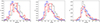 |
Fig. 5. Same as Fig. 4, but for K2-GALAH. |
| In the text | |
|
Fig. 6. [C/N] ratio. Left panel: histogram for [C/N] of the stars in our K2 sample (gray, blue, and red histograms represent the low-α, old high-α, and young α-rich samples, respectively). Middle panel: [C/N] vs. mass for the stars in our sample, with colors as in the left panel. The solid lines represent the predictions of stellar evolution models from Vincenzo et al. (2021) at different metallicities ([Fe/H] = −1 in yellow, −0.5 in green, and +0.25 in purple). Right panel: [C/N] ratios for the entire sample color-coded by [Fe/H] (as indicated in the color scale). In this panel are shown low-α (dots), old high-α (triangles), and young-α rich stars (bigger dots). |
| In the text | |
|
Fig. 7. Distribution function of guiding radii Rg (left panel), Zmax (middle panel), and eccentricity (right panel) for the different populations considered: young α-rich (in red), old high-α (blue), low-α (gray). |
| In the text | |
Current usage metrics show cumulative count of Article Views (full-text article views including HTML views, PDF and ePub downloads, according to the available data) and Abstracts Views on Vision4Press platform.
Data correspond to usage on the plateform after 2015. The current usage metrics is available 48-96 hours after online publication and is updated daily on week days.
Initial download of the metrics may take a while.