| Issue |
A&A
Volume 683, March 2024
|
|
|---|---|---|
| Article Number | A74 | |
| Number of page(s) | 13 | |
| Section | Galactic structure, stellar clusters and populations | |
| DOI | https://doi.org/10.1051/0004-6361/202244157 | |
| Published online | 08 March 2024 | |
The Prince and the Pauper: Evidence for the early high-redshift formation of the Galactic α-poor disc population⋆,⋆⋆
1
Max-Planck Institute for Astronomy, 69117 Heidelberg, Germany
e-mail: This email address is being protected from spambots. You need JavaScript enabled to view it.
2
Ruprecht-Karls-Universität, Grabengasse 1, 69117 Heidelberg, Germany
3
Mullard Space Science Laboratory, University College London, Holmbury St. Mary, Dorking, Surrey RH5 6NT, UK
4
Institut de Ciencies del Cosmos (ICCUB), Universitat de Barcelona (IEEC-UB), Martii i Franques, 1, 08028 Barcelona, Spain
5
Institute of Space Sciences (ICE, CSIC), Carrer de Can Magrans s/n, 08193 Cerdanyola del Valles, Spain
6
Institut Estudis Espacials de Catalunya (IEEC), Carrer Gran Capita 2, 08034 Barcelona, Spain
7
Institute for Astronomy, University of Edinburgh, Royal Observatory, Blackford Hill, Edinburgh EH9 3HJ, UK
8
Institute of Astronomy, University of Cambridge, Madingley Road, Cambridge CB3 0HA, UK
9
Niels Bohr International Academy, Niels Bohr Institute, University of Copenhagen, Blegdamsvej 17, 2100 Copenhagen, Denmark
10
Universität Heidelberg, Interdisziplinäres Zentrum für Wissenschaftliches Rechnen, Im Neuenheimer Feld 205, 69120 Heidelberg, Germany
11
Universität Heidelberg, Zentrum für Astronomie, Institut für Theoretische Astrophysik, Albert-Ueberle-Straße 2, 69120 Heidelberg, Germany
Received:
31
May
2022
Accepted:
28
November
2023
Abstract
Context. The presence of [α/Fe]–[Fe/H] bi-modality in the Milky Way disc has intrigued the Galactic archaeology community over more than two decades.
Aims. Our goal is to investigate the chemical, temporal, and kinematical structure of the Galactic discs using abundances, kinematics, and ages derived self-consistently with the new Bayesian framework SAPP.
Methods. We employed the public Gaia-ESO spectra, as well as Gaia EDR3 astrometry and photometry. Stellar parameters and chemical abundances are determined for 13 426 stars using NLTE models of synthetic spectra. Ages were derived for a sub-sample of 2898 stars, including subgiants and main-sequence stars. The sample probes a large range of Galactocentric radii, ∼3 to 12 kpc, and extends out of the disc plane to ±2 kpc.
Results. Our new data confirm the known bi-modality in the [Fe/H]–[α/Fe] space, which is often viewed as the manifestation of the chemical thin and thick discs. The over-densities significantly overlap in metallicity, age, and kinematics and none of them offer a sufficient criterion for distinguishing between the two disc populations. In contrast to previous studies, we find that the α-poor disc population has a very extended [Fe/H] distribution and contains ∼20% old stars with ages of up to ∼11 Gyr.
Conclusions. Our results suggest that the Galactic thin disc was in place early, at lookback times corresponding to redshifts of z ∼ 2 or more. At ages of ∼9 to 11 Gyr, the two disc structures shared a period of co-evolution. Our data can be understood within the clumpy disc formation scenario that does not require a pre-existing thick disc to initiate the formation of the thin disc. We anticipate that a similar evolution can be realised in cosmological simulations of galaxy formation.
Key words: Galaxy: abundances / Galaxy: disk / Galaxy: fundamental parameters / Galaxy: structure
Full tables of Teff, log g, NLTE [Fe/H], [Mg/Fe], Vmic Ages, and uncertainties are available at the CDS via anonymous ftp to cdsarc.cds.unistra.fr (130.79.128.5) or via https://cdsarc.cds.unistra.fr/viz-bin/cat/J/A+A/683/A74
Based on observations made with the ESO/VLT, at Paranal Observatory, under program 188.B-3002 (The Gaia-ESO Public Spectroscopic Survey, PIs: G. Gilmore and S. Randich). Also based on observations under programs 171.0237 and 073.0234.
© The Authors 2024
 Open Access article, published by EDP Sciences, under the terms of the Creative Commons Attribution License (https://creativecommons.org/licenses/by/4.0), which permits unrestricted use, distribution, and reproduction in any medium, provided the original work is properly cited.
This article is published in open access under the Subscribe to Open model.
Open access funding provided by Max Planck Society.
1. Introduction
The structure and evolution of the Galactic disc are still among the most complex problems investigated in studies of Galaxy formation. Since the discovery of the thick disc (Gilmore & Reid 1983), much work has been focused on the bi-modality in the space of chemical abundances (e.g. Bensby et al. 2005; Reddy et al. 2006; Bovy et al. 2012; Recio-Blanco et al. 2014; Duong et al. 2018). Many studies based on stars in the solar neighbourhood and beyond pointed out the existence of two populations, [α/Fe]-rich and [α/Fe]-poor, partly overlapping in metallicity (e.g. Fuhrmann 1998; Nidever et al. 2014; Guiglion et al. 2024), age (e.g. Bensby et al. 2014; Feuillet et al. 2019), and kinematics (e.g. Ruchti et al. 2011; Lee et al. 2011; Kordopatis et al. 2011; Hayden et al. 2015). These stellar populations have been deemed as the “thin” and the “thick” disc, and their morphological parameters have since then been subject of a major interest (Bland-Hawthorn & Gerhard 2016). It has been shown that different physical processes may influence the formation and evolution of sub-structure in the disc, including multiple infall (e.g. Chiappini et al. 1997; Spitoni et al. 2019), radial migration (e.g. Schönrich & Binney 2009a,b; Loebman et al. 2011; Minchev et al. 2013), and radial mixing caused by satellites (Quillen et al. 2009), growth induced by mergers (e.g. Villalobos & Helmi 2008; Read et al. 2008; Villalobos et al. 2010), gas-rich accretion and mergers (e.g. Brook et al. 2004; Stewart et al. 2009; Grand et al. 2018; Buck 2020), local gas instabilities in discs associated with turbulence (e.g. Noguchi 1999; Bournaud et al. 2009; Clarke et al. 2019), dynamical interaction with cold dark matter sub-halos (Hayashi & Chiba 2006; Kazantzidis et al. 2009), galactic winds (Moster et al. 2012), and early outflows (Khoperskov et al. 2021). It has also been demonstrated that the chemical bi-modality is a relatively rare phenomenon in L* galaxy discs (Mackereth et al. 2018; Gebek & Matthee 2022), but we refer to Khoperskov et al. (2021) for more details on this topic. More recent studies address the spatial variability of the bi-modality (Hayden et al. 2015; Bovy et al. 2016; Nandakumar et al. 2022) in greater detail, finding that [α/Fe]-rich component is more centrally concentrated, whereas the [α/Fe]-poor component has a larger radial extent (Haywood et al. 2019; Sahlholdt et al. 2022). Therefore, the question of whether the populations are indeed distinct stellar components with a separate formation history still remains open.
In this work, we perform of a detailed analysis of the chemical, temporal, and kinematical distribution functions of the Galactic disc populations, using data from the Gaia-ESO survey and Gaia. The key difference between the Gaia-ESO and other comparable medium- and high-resolution stellar surveys, RAVE, APOGEE, and GALAH, is its photometric coverage. Most stars in the Gaia-ESO selection are rather faint (14 ≲ Gmag ≲ 18 mag), and as outlined in Gilmore et al. (2012), Randich et al. (2013), Stonkutė et al. (2016) this selection allows to uniquely address the parameter space of the inner and outer thin and thick disc, and the thick disc to halo transition, beyond what is possible with brighter and more local samples.
The paper is organised as follows. In Sect. 2, we discuss the observational sample. Section 3.1 outlines the approach used for the determination of stellar parameters and chemical abundances. In Sect. 3.2, we briefly state how the ages are determined. Section 3.3 deals with the validation of stellar parameters and ages. Results are presented in Sect. 4, with a focus on the distributions of chemical abundances, combined with kinematics and ages. Furthermore, we discuss the results in the context of previous observational and theoretical findings. We present our conclusions in Sect. 6.
2. Observations
In this work, we rely on targets observed within the Gaia-ESO large spectroscopic survey (Gilmore et al. 2012, Randich et al. 2013). In the latest public data release (DR4), spectra for over 105 were made available, and here we use all spectra taken with the HR10 setting of Giraffe spectrograph1. The HR10 data are available for 55 761 stars. The signal-to-noise (S/N) distribution of the sample is very broad and ranges from 2 to a few 100 per pixel.
Figure 1 shows the targets in the photometric colour-magnitude (CMD), J versus J − Ks, plane, where J and Ks are VISTA photometric filters (McMahon et al. 2013). The apparent regular distribution is caused by the photometric selection of targets in the input Gaia-ESO catalogue. For the Giraffe catalogue, the following basic selection scheme was used: 0.00 ≤ (J − Ks)≤0.45 and 14.0 ≤ J ≤ 17.5 for the blue box, and 0.40 ≤ (J − Ks)≤0.70 and 12.5 ≤ J ≤ 15.0 for the red box. The boxes were defined to maximise the probability of observing targets in all Galactic components, the discs and the halo; therefore, the target densities vary drastically and to account for this effect, the boxes were slightly extended in order to optimise the fiber occupancy in each field. In particular, in the fields where number of targets exceeded the number of fibers (as in low latitude fields), additional selection criteria were used, such as shifting the boxes by the mean value of extinction in a given field 0.5 E(B − V). This procedure leads to a characteristic spread of the distribution along the x-axis, as seen in Fig. 1. The relative distribution is such that the majority of targets (80%) are in the blue box, whereas stars in the red box account for about 20% of the sample. The blue box targets include main-sequence, turnoff, and subgiant stars, and the red box was optimised for red clump stars; however, because of the extension of the boxes a certain overlap exists. For the detailed description of the input catalogue, we refer to Stonkutė et al. (2016). We note that this selection implies that most targets in the Gaia-ESO HR10 sample are much fainter, 14 ≲ Gmag ≲ 18 mag, compared to other surveys such as RAVE, APOGEE, or GALAH. The selection also has a strong effect on the properties of our sample, in the plane of astrophysical parameters. Specifically (see e.g. Bergemann et al. 2014; Thompson et al. 2018), the distribution of our sample is preferentially skewed towards older populations with slightly sub-solar metallicities and we explore this issue in more detail in Sect. 3.4.
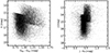 |
Fig. 1. Photometry of the observed sample. Left panel shows the distribution in the Gaia magnitudes, G vs. GBP − GRP. Right panel shows the distribution in the VHS magnitudes, J vs. J − Ks (see Sect. 2). |
We complement these data with the proper motions, photometry, and extinction from the EDR3 Gaia catalogue (Gaia Collaboration 2021). The cross-match between every Gaia-ESO spectrum and Gaia ED3 catalogue was performed on grounds of angular position within a 1.0 arcsec tolerance (cone search). Distances and their uncertainties were adopted from Bailer-Jones et al. (2021). The spatial distribution of the sample is shown in Fig. 2. Most of these objects are confined closer to the plane with altitudes of up to 2 kpc and they probe a range of Galactocentric radii from ∼5 to 12 kpc. The 3D space velocities2 for the sample are calculated using the Python package “astropy” (Astropy Collaboration 2013, 2018). The accuracy of the astrometric information is high enough to yield the velocities with an uncertainty of ≲5 km s−1.
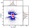 |
Fig. 2. Spatial distribution of the observed sample. The vertical axis represents the height above the disc plane in kpc and the horizontal represents the Galactocentric radius in kpc. The colour scale shows normalised density from 0.07% (dark blue) to 100% (dark red). |
3. Methods
3.1. Stellar parameters
The homogeneity, accuracy, and precision of stellar parameters is essential given by the scientific goals of this study. However, our analysis of the Gaia-ESO sixth internal data release (iDR6)3 (Gilmore et al. 2012; Randich et al. 2013) shows artificial ridges and bifurcations in the space of stellar parameters and their uncertainties. It suffers from some loss of precision owing to the complex homogenisation and cross-calibration procedure employed. Therefore, this does not allow for a robust analysis of the distribution functions in the space of astrophysical parameters and ages.
We have therefore opted to re-analyse the spectra using the Bayesian SAPP pipeline described in Gent et al. (2022). This method was shown to provide atmospheric parameters, including Teff, log g, [Fe/H], and abundances (Mg, Ti, Mn), across a broad range of stellar parameters: 4000 ≲ Teff ≲ 7000 K, 1.2 ≲ log g ≲ 4.6 dex, and −2.5 ≲ [Fe/H] ≲ +0.6 dex. Extensive tests of the NLTE synthetic spectral grids and the Payne model (Ting et al. 2019) based on these can be found in Kovalev et al. (2019). The latter study also presented a detailed spectroscopic analysis of the benchmark stars, including main sequence stars, subgiants, and red giants, and 742 stars probing the entire evolutionary sequence in 13 open and globular clusters. In Gent et al. (2022), the code was developed to carry out the full Bayesian analysis, by combining the probabilities obtained from the spectroscopy, photometry, astrometry, and asteroseismic data analysis modules.
The results of the SAPP analysis are shown in Fig. 3, where the entire Gaia-ESO HR10 sample with S/N > 20 is plotted in the Teff − log g plane. In total, we have 13 426 stars with reliable stellar parameters The characteristic uncertainties of stellar parameters are of the order 51 K for Teff, 0.04 dex for log g, 0.05 dex for [Fe/H], 0.06 dex for [Mg/Fe]. These uncertainties represent the combined estimates derived from the shape of the multi-dimensional posterior PDF; thus, they account for the statistical uncertainties (those of the observed data) and for the systematic (differences between the individual PDFs derived from the photometric, astrometric, and spectroscopic data). For more details on the error analysis, we refer the reader to Gent et al. (2022).
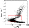 |
Fig. 3. Distribution of the observed sample in the Teff − log g plane. The targets enclosed within the red box represent the sample used for the analysis of ages. |
3.2. Stellar ages
One important component of this study is the availability of ages. Ages are derived using the Bayesian pipeline BeSPP presented in Serenelli et al. (2013), which was also applied to the analysis of the first Gaia-ESO data release in Bergemann et al. (2014). The code relies on the GARSTEC grid of stellar evolutionary tracks Weiss & Schlattl (2008; also used in SAPP) that covers the mass range from 0.6 to 5.0 M⊙ with a step of 0.02 M⊙ and metallicity from −2.50 to +0.60 with a step of 0.05 dex. The spectroscopically derived [α/Fe] ratio is taken into account for the age determinations by modifying the derived [Fe/H] following the prescription [Fe/H] → [Fe/H] + 0.625 [α/Fe], which agrees with the traditionally used modification by Salaris et al. (1993) within 10% in the range −0.45 < [α/Fe] < +0.45.
The analysis of ages is limited to subgiants and upper main-sequence stars (including turn-off, TO), because of the strong degeneracy typically identified between tracks of different ages and metallicities for the lower MS and RGB phases. This selection is made by limiting the effective temperature and surface gravity to: 4700−6700 K, 3.5−4.5 dex for subgiants and turn-off stars, and 5400−6700 K, 3.5−4.2 dex for the upper main-sequence. We also include the stars with accurate abundances and ages analysed in Bergemann et al. (2014). These stars are part of the Gaia-ESO sample. We further limit our sample with a maximum of 0.1 dex in [Fe/H] error. The uncertainties of stellar parameters are small enough to ensure that our selection retains most of the subgiants in the sample and it minimises the contamination by lower main-sequence stars.
In the next section, we describe the validation of our stellar parameters and ages using different inputs and methodological approaches. We then present the final sample with accurate ages that is used for the analysis of the properties of the Galactic disc.
3.3. Validation of parameters
The quality of stellar parameters is important within the scope of this paper. In Paper I (Gent et al. 2022), we presented a careful validation of our stellar analysis pipeline and its outputs (including metallicities, masses, and ages), using a sample of benchmark stars with independently determined stellar parameters, including interferometic Teff and ages constrained by asteroseismology. We showed that a combination of spectroscopy, astrometry, and photometry in the Bayesian framework yields metallicities accurate to 0.02 dex and ages with the precision of ∼0.6 and accuracy of ∼1 Gyr, in line with results of similar earlier studies (e.g. Serenelli et al. 2013; Schönrich & Bergemann 2014). While the focus of our work in Paper I was on main-sequence stars and subgiants and based on the same type of observational information (i.e. Gaia-ESO spectra, Gaia photometry and astrometry), the difference here is the use of global asteroseismic quantities that are not available for the majority of stars in the present sample.
Therefore, we present additional tests in order to investigate the properties of data errors in the parameter space that is relevant to our investigation. First, we carried out an analysis of the atmospheric parameters of stars using the infra-red flux (IRFM) method (Casagrande et al. 2010, 2021). The results obtained by applying the IRFM technique to our main sample are provided in Table 1. The effective temperatures are in agreement with the reference SAPP values to 16 ± 52 K, whereas the resulting surface gravities and metallicities change by −0.06 ± 0.14 dex and 0.01 ± 0.04 dex, respectively, if Teff is derived from IRFM instead of spectroscopy. We also investigated the quality of surface gravities calculated by the SAPP by applying a systematic shift to distances adopted from Bailer-Jones et al. (2021). The shift was estimated through the analysis of typical uncertainties of distances: the average distance error in our sample is of the order 8% pc with the majority of stars having the error of ∼5%. The resulting stellar parameters calculated with the offset distances are also provided in Table 1. The shift has no significant effect on Teff, with the average difference of 2 K and a scatter of 12 K, whereas surface gravities and metallicities are affected at the level of 0.00 ± 0.08 dex and 0.00 ± 0.02 dex, respectively.
Sensitivity of the astrophysical parameters of the stellar sample to changes in the input data and in methodology (see text).
In the third step, we explore the sensitivity of ages to the methodology by performing the analysis of ages using an alternative approach presented in Xiang & Rix (2022), where only Ks magnitudes were used circumventing the need for surface gravities. In the latter case, we make use of either only Ks, or Ks and J magnitudes from 2MASS and the synthetic photometry. Comparing the resulting ages with the ages calculated self-consistently within the Bayesian framework, we find that the effect on ages is maximum at slightly sub-solar metallicities, with the bias and scatter of ∼0.9 Gyr and ∼2.2 Gyr, respectively. Interestingly, more metal-poor stars, [Fe/H] ≲ −0.7 dex, are least affected by the choice of the method, with the age bias of only 0.3 Gyr and scatter of 1.4 Gyr. Finally, we compare the ages obtained using BeSPP with the age estimated by the SAPP, following Gent et al. (2022). Since the codes assume a similar algorithm, the same input data and evolutionary tracks, this comparison primarily demonstrates the internal precision of ages. We find the both codes are in excellent agreement, with a 0.5 Gyr bias and a scatter of 0.4 Gyr. Based on these tests, we select only those stars for which the ages are consistent to better than 1 Gyr, obtained with both methods and with both codes, yielding a final sample of 2898 stars with the characteristic uncertainty of ages ranging from 0.7 to 2 Gyr and the mean error of 1.3 Gyr.
3.4. Survey selection function
In order to assess the influence of the survey selection function on our data set, we followed the methodology of Bergemann et al. (2014) and Thompson et al. (2018). To ensure self-consistency in the analysis, the same evolutionary tracks were used (see Sect. 3.2). First, a complete population of stars was generated assuming the Salpeter initial mass function, a constant star formation rate, and a uniform and age-independent metallicity [Fe/H] distribution. This [Fe/H] population exhibits a trend, which reflects simply the IMF and the stellar evolution lifetime, that is shorter at lower [Fe/H] and same mass. We then removed stars outside the Teff − log g box used in our analysis (Sect. 3). In the second step, this Mock dataset is used to determine the completeness fraction by calculating the ratio of photometrically selected targets relative to the complete sample. This is done separately for the blue and red photometric boxes.
Figure 4 shows for a given distance of 1 kpc, the relative stellar density (left) and completeness (right) of the Mock stellar population from the red and blue selection boxes. The distance was chosen as representative of the bulk fraction of stars in the observed Gaia-ESO sample, but careful inspection of the simulated fractions suggests that the distribution is qualitatively similar at distances at 0.5 kpc or 2 kpc. It may be concluded that the distribution of stars in the age-metallicity plane suffers from a systematic bias, which is primarily caused by the colour cuts adopted in the Gaia-ESO survey. These cuts lead to a very pronounced depletion in the fraction of young stars with ages ≲7 Gyr, although the effect slightly depends on metallicity. The red box additionally skews the distribution towards old metal-rich stars, whereas the blue box is primarily sensitive to old metal-poor stars. This situation is rather similar to the completeness case of the Gaia-ESO UVES sample described by Bergemann et al. (2014) and Thompson et al. (2018).
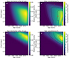 |
Fig. 4. Synthetic stellar population to simulate the selection effect of Gaia-ESO survey and of the observed stellar sample. Here, the results of the simulation at 1 kpc are shown for the blue box (top row) and red box (bottom row), as defined in Sect. 2. Right: completeness fraction, defined as the ratio of stars with cut to the number of stars without cut, that is, the larger the number the more stars are retained in the population after applying the colour cuts (Sect. 2). In case of no bias, the completeness fraction is unity 1. |
4. Results
4.1. Chemical abundances
The [Mg/Fe] abundance ratios of our sample against metallicity are shown in Fig. 5. The number of stars with reliable abundances is the same sample as Sect. 3.1. is Here, we limited the analysis of [α/Fe] to the abundance of Mg, because no particular sub-structure is visible in the distribution of Ti or Mn abundance ratios. We also note that Mg is a key α element produced by α capture reactions during the hydrostatic C and Ne burning phases in massive stars (Clayton 1968; Woosley & Weaver 1995). Therefore, it is reasonable to adopt the notation of Mg as a representative of the α-group.
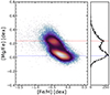 |
Fig. 5. Densities of NLTE abundances of [Mg/Fe] as a function of [Fe/H]. The dashed lines represent the average [Mg/Fe] value for stars which are α-rich (red) and α-poor (blue). |
As previous studies have shown, we also see a prominent bi-modality in the [Mg/Fe] abundance ratios, which is manifested as two over-densities separated at [Mg/Fe] ≈ +0.15 dex across the entire metallicity range, −1.5 ≈ [Fe/H] ≈ −0.2 dex. The low-α component peaks at [Mg/Fe] ≈ +0.05 dex and the high-α component at [Mg/Fe] ≈ +0.24 dex. It shall be stressed that no component of the analysis, neither the observed data (spatial distribution) nor the grid (models), have any known non-linear dependence that could lead to this discontinuity in the space of Mg and Fe abundances. In particular, in the spectroscopic grid used in the chemical abundance analysis, all elemental abundances have a random uniform distribution. In agreement with the visible over-densities, we chose to assign stars to the α-rich population if their associated [Mg/Fe] abundance was above 0.13 dex and to the α-poor disc otherwise. Throughout the text, we refer to these two sets of stars “α-rich” and “α-poor” populations, respectively.
Comparing our distributions with the literature, we find an overall satisfactory agreement, although it should be noted that owing to a combination of factors, including vastly different spatial-photometric coverage of observational surveys, their observational strategies, and incomplete volume sampling, certain differences arise that render a one-to-one comparison of chemical abundances in a given volume of the Galaxy impossible. Nonetheless, it appears that our distributions are consistent with the distributions seen in the previous DRs of the Gaia-ESO (e.g. Mikolaitis et al. 2014; Recio-Blanco et al. 2014; Kordopatis et al. 2015; Guiglion et al. 2015), as well as independent studies (e.g. Adibekyan et al. 2013; Bensby et al. 2014). In the latter work, a prominent separation is detected in [Ti/Fe] abundance ratios, whereas the [Mg/Fe] ratios show a more continuous distribution. This could be a consequence of the spatial coverage of the sample. The study by Bensby et al. focuses on the nearby stars in the solar neighbourhood, whereas our sample probes more extended regions in the Rgc − z space, reaching 3 < Rgc < 13 kpc and |z|≈ ± 3 kpc. A similar distribution of the low and high-α/Fe populations is seen in the APOGEE sample (e.g. Hayden et al. 2015). We should note, however, that their α parameter refers to the average of different elements4, and so their distributions are not directly comparable to the present sample. The GALAH survey results (Bland-Hawthorn et al. 2019; Buder et al. 2021) are also consistent with our distributions. In the chemical distributions of the RAVE stellar sample (Steinmetz et al. 2020), the α-rich component is discernible at [α/Fe] ≈ +0.45, which is somewhat higher compared to our data and the samples from APOGEE5 (Hayden et al. 2015; Jönsson et al. 2020), although they are consistent within the uncertainties of both samples.
4.2. Kinematics and abundances
For our kinematic analysis, we used a right-handed Galactocentric cylindrical coordinate system, where the velocity component Vr points towards the Galactic centre, Vϕ in opposition direction of the rotation, and Vz vertically down out of the disk. By converting RA, Dec and proper motions to Galactocentric coordinate frames executed by python package “astropy” (Astropy Collaboration 2013, 2018), we derived the Cartesian Galactocentric coordinates and velocities. Thus, we obtain:
 (1)
(1)
 (2)
(2)
where  . We used Solar Galactocentric coordinates, r⊙ = (X⊙, Y⊙, Z⊙)T = (−8.122, 0, 0)T kpc and v⊙ = (U⊙, V⊙, W⊙)T = (11.1, 12.24, 7.24)T km s−1 (Schönrich et al. 2010), thus defining the Solar Galactocentric radius as R = 8.122 kpc (Drimmel & Poggio 2018). Then, VX = U, and VY = V + Vc, ⊙, where Vc, ⊙ is the circular velocity value at Solar radius = 233.4 km s−1 (Drimmel & Poggio 2018)6.
Figure 6 shows the distribution of our α-poor and α-rich samples in the plane of radial velocity, Vr, versus azimuthal velocity, Vϕ, for different metallicity bins. The kinematic quantities were calculated using the positions, proper motions, and parallaxes from Gaia DR3 and the astropy package.
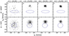 |
Fig. 6. Phase-space of the observed Gaia-ESO sample: azimuthal velocity, Vϕ, versus radial velocity, Vr, coloured in density. The upper panels represent the α-poor population, and the lower panels represent the α-rich population. Each population is split into two [Fe/H] bins: metal-poor and metal solar-rich. The blue ellipse represents the halo distribution following the multi-Gaussian approach described in Belokurov et al. (2018) to determine halo contamination within the disc. |
It can clearly be seen that the majority of stars from both α-rich and α-poor populations are centred with Vr ≃ 0 km s−1 and Vϕ ≃ 220 km s−1, consistent with the expectations for the Galactic disc (Ruchti et al. 2011; Navarro et al. 2011; Bensby et al. 2014). With decreasing metallicity, the velocity dispersion in the radial direction increases, the mean rotation of stars decreases, and a counter-rotating component appears at [Fe/H] ≈ −0.6, which is in line with previous studies of the disc (Chiba & Beers 2000; Fuhrmann 2004; Deason et al. 2017). Perhaps the most interesting feature of the observed distributions is the presence of a significant fraction of metal-poor, −1 ≲ [Fe/H] ≲ −0.6, and α-poor stars on disc orbits. In terms of kinematics, these stars are identical to the more metal-rich α-poor population suggesting their thin disc origin. In Sect. 4.3, we describe our more detailed analysis of this group in terms of their integrals of motion to better understand their properties. In the most metal-poor bin, [Fe/H] ≲ −1 dex, low-Vϕ stars with large radial velocities |Vr|≳200 km s−1 appear. This population resembles the low-α metal-poor accreted halo component, which was identified in smaller targeted samples (e.g. Nissen & Schuster 2010) and subsequently confirmed with other datasets (Bergemann et al. 2017; Hayes et al. 2018; Haywood et al. 2018). Belokurov et al. (2018) identified these stars as a population associated with a massive merger event around 8 to 11 Gyr ago, which was subsequently coined as the Gaia-Sausage (Myeong et al. 2018) or the Gaia-Enceladus event (Helmi et al. 2018).
Combining Gaia DR2 with APOGEE, Di Matteo et al. (2019) found that the accreted halo component is characterised by Vϕ ≈ 0 km s−1 and is approximately Gaussian distributed in Vr, with the corresponding velocity dispersion of ≈120 km s−1 (Lancaster et al. 2019). For highly prograde velocities, Vϕ > 100 km s−1 (Di Matteo et al. 2019, their Fig. 10) however, the contribution of the accreted halo population is of the order of a few percent. We estimated the contamination by the halo stars in our sample following the multi-Gaussian decomposition approach from Belokurov et al. (2018). The model estimates are performed separately for the α-poor and the α-rich populations. In short, we selected all stars with Vϕ < 0 and any Vr value and we modelled the bivariate distribution of Vϕ and Vr by a Gaussian that is centred on Vϕ = 0. This resulting bivariate Gaussian function is assumed to represent the halo component of the entire stellar sample. Then, the resulting contamination fraction is calculated as the ratio of the number of stars in this Gaussian to to the total number of stars above a given Vϕ value. In Table 2, we show the resulting expected fractions of the contamination of our sample by halo stars, as predicted by our model for both α populations. Similar to Di Matteo et al. (2019), we find the lowest value of this range to be ∼110 km s−1 (Fig. 6). For Vϕ above this limit, the contamination by the halo is expected to be at the level of < 1% for the α-poor population, as long as [Fe/H] ≳ −1. For the most metal-poor bin, [Fe/H] ≲ −1, the contamination is ∼12%. In the α-rich population, the fractions are not too different in the metallicity bins [Fe/H] ≳ −1. However, as expected, the halo component becomes dominant over the disc for the most metal-poor α-rich bin.
Contamination of the observed sample by halo stars in % (see text).
In addition, we computed the halo contamination through a slightly different model independent procedure described in detail in Appendix A, where instead of fitting the Vϕ distribution, we calculated the contamination at Vϕ velocities in individual [Fe/H] bins by reflecting the Vϕ distribution across Vϕ = 0. The results of this calculation (Fig. A.1) confirm the decomposition based on Belokurov et al. (2018), suggesting that above [Fe/H] ≳ −1, the observed stellar sample is primarily represented by stars with disc-like kinematics, and the contribution of accreted halo stars is marginal (see also Ruchti et al. 2011). It is therefore safe to assume that stars above this metallicity with Vϕ ≳ 110 km s−1 are representative of the Galactic disc. Consequently, we rely on this criterion to define the disc sample and use this in combination with the criteria to separate α-poor and α-rich populations (Sect. 4.1) to investigate the evolutionary properties.
4.3. Orbital characteristics
In order to further understand the dynamical properties of our chemically distinguished samples and to better characterise the old α- and metal-poor sample, we took a step further and looked at their action distribution. In principle, actions and their corresponding angles are just another set of canonical coordinates. However, for non-resonant orbits in axisymmetric potentials the actions are defined as the constants of motion, invariant under adiabatic changes and even mostly invariant under radial migration. Furthermore, in those potentials, the three conserved actions Jϕ, Jr, and Jz correspond to our directions in cylindrical coordinates and have an intuitive meaning: Jϕ is equal to specific angular momentum Lz; JR and Jz are a measure of the radial, respectively, vertical, excursion of the orbit around its guiding centre radius, Rg, and the galactic plane. Hence, using actions (by definition) allows us to fully classify any orbit by just three parameters. To obtain actions for our stellar sample, we used the Agama (Vasiliev 2019) code with the Galactic potential from McMillan (2017). In order to minimise the noise from distance errors, we introduce a parallax cut of 10% that reduces our full chemo-dynamical sample to 11 137 stars.
Figure 7 shows the resulting action distributions in Jr and Lz, where we distinguish between the halo population, as identified kinematically in Sect. 4.2, as well as the α-poor and the α-rich disc components defined chemically (see Sect. 4.1). We also overplot the entire chemo-dynamical sample, and additionally highlight the other interesting sub-group: the metal-poor α-poor sample, namely, stars with [Fe/H] < −0.5 and [α/Fe] < +0.13. We find that both disc populations have their maximum value around zero value of Jr and that they are roughly exponentially distributed as expected by a pseudo-isothermal distribution function (Carlberg & Sellwood 1985; Binney 2010). They do show different exponential factors though, with the α-poor disc characterised by a larger, more negative factor corresponding to the mean radial action in the sample  . This lower spread in Jr implies that the α-poor stars are on radially less eccentric orbits than the α-rich ones, namely, the α-poor sample is kinematically colder and on more circular orbits. This is the reason for the often used identification between the chemically defined alpha-poor disc and the kinematically defined thin disc. The disc stars in our sample have |Lz| values that tend to be slightly lower compared to the solar value at about 2000 kpc km s−1. The α-rich disc population shows somewhat lower |Lz|, that is, it is dominated by stars on orbits with guiding centre radius further in the inner disk. This is a result of the shorter scale length of the α-rich with respect to the α-poor disc (Bensby et al. 2011; Cheng et al. 2012).
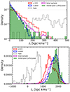 |
Fig. 7. Density distribution in actions Jr and Lz for our identified components. The black line in the lower panel represents the Solar Lz value of 1995 kpc km s−1. |
The α-poor disc in Fig. 7 has a very narrow distribution around Lz ≈ 1800 kpc km s−1 and it is skewed towards the larger values. The Lz distribution of the α-rich disc peaks at ≈1300 to 1400 kpc km s−1 with a larger spread than the α-poor disc. Similar distributions were reported by Bland-Hawthorn et al. (2019) and Gandhi & Ness (2019). The latter analysis suggests that the α-poor and the α-rich sequences have Lz range in ≈1800 to 2100 kpc km s−1 and ≈1600 to 1750 kpc km s−1, respectively, over a range of ages (their Fig. 6). The overall orbital properties of the disc are also close to those reported by Trick et al. (2019), ∼1760 kpc km s−1, and to Buder et al. (2021). Trick et al. (2019) used Gaia data, whereas our data based on the VLT spectra, thus, there are more stars with lower Rg and a limited |Lz| range. The study Buder et al. (2021) does not distinguish between α-rich and α-poor in the kinematic analysis, the Lz distribution of our total disc sample peaks at 1800 kpc km s−1 with an average value at ≈1700 kpc km s−1, which is consistent with their findings of the dominant fraction of stars with radial actions similar to the solar value. We note, however, that the GALAH sample is significantly brighter (9 ≳ V ≳ 14), and it is therefore more local compared to the Gaia-ESO. In addition (Sect. 2), the Gaia-ESO sample, owing to its photometric selection function, is somewhat biased against young stars with ages < 7 Gyr, which make up a major fraction of the Galactic disc. We would therefore expect a better completeness of the thin disc in the GALAH distribution.
One particularly interesting feature of our sample is the presence of the α-poor and metal-poor disc component. This component follows quite closely the Jr and Lz distribution of the α-poor disc. Furthermore, with the exception of ten stars, all of these stars (524 stars with parallax-over-parallax-error cut of 10) are neither in the Lz nor at the high Jr region that could be considered the Galactic halo, and their distribution is also not representative of that of the α-rich disc. We carefully checked the observed data, as well as the stellar parameters and kinematic quantities, but we did not find any evidence for a systematic error that could possibly lead to a misclassification in terms of the population membership. The only distinct feature of this population is that it is concentrated at slightly higher |Lz| values compared to the thin disc sample, which could possibly indicate that those are stars that formed in the outer disc and have since migrated inwards. However, currently we do not have any other means to provide a robust test of their origins.
Interestingly, evidence for a kinematically cold α-poor and metal-poor disc population can also be seen in the analysis of the GALAH survey data by Bland-Hawthorn et al. (2019). Their distributions suggest that for stars with [Fe/H] < −0.5 dex, the average Lz is slightly higher than that of the average disc, closer to 1950 kpc km s−1, which is in good agreement with our results. Xiang & Rix (2022) found a non-negligible fraction of α-poor metal-poor stars with Lz > 1500 kpc km s−17 and ages from 5 to 9 Gyr. This study came to a similar conclusion that this component may arise from stars that were born further out and subsequently migrated inwards. The origin of metal-poor α-poor stars in the outer disc was also suggested by Haywood et al. (2013), Buder et al. (2019), and Wu et al. (2021).
4.4. Ages and abundances of disc stars
Finally, we explore the distribution of the two [α/Fe] components with respect to stellar age. This analysis is limited to the final sample in order to avoid spurious trends caused by imprecise stellar parameters. Because of the very strong impact of the survey selection function on the completeness and statistical properties of younger populations (see Sect. 3.4), we did not explore the full age distributions. Instead, we limited the analysis to the relative behaviour of old stellar components in the α-poor and α-rich sample. This choice was motivated by the fact that our samples appear to be rather complete only for ages in excess of ≈9 Gyr. Therefore, this limit is used in Fig. 8 to show the fraction of very old stars in each α component to the total number of stars in the respective population against metallicity. In addition to the analysis of ages, we derived the relative fraction of stars with redshift (z) in excess of ∼2. This is driven by the peak epoch of star formation across the universe (Madau & Dickinson 2014), to quantify the fraction of stars in both α sequences to investigate early formation of the Milky Way disc.
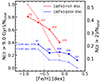 |
Fig. 8. Number of stars (vertical axis) older than 9 Gyr with respect to the total number (annotated as text) of α-poor, rich stars (respectively) in a given [Fe/H] bin. Grey dotted lines represent [Fe/H] bin boundaries. Blue data represents α-poor stars, red data represents α-rich stars. The solid lines represent the left y-scale: fraction of stars with ages (τ) more than 9 Gyr, the dashed lines represent the right y-scale: fraction of stars with redshift (z) more than 2. |
To derive the redshift, ages were converted to z using the python module astropy.cosmology. The cosmology chosen is the Flat Λ-CDM model based Planck satellite data (Planck Collaboration XIII 2016) with a Hubble constant of H0 = 67.7 km s−1 Mpc−1 and a fraction of observed density to critical density of Ω = 0.307. We chose this to be consistent with IllustrisTNG simulations (Nelson et al. 2019).
It is interesting that both components of the Galactic disc (and especially the α-poor component) show a significant fraction of old stars at any [Fe/H]. As seen in Fig. 8, the fraction levels at ≈20% at solar and slightly sub-solar metallicities, but it grows with decreasing [Fe/H] peaking at 37% for τ > 9 Gyr and 18% for z > 2. For the α-rich disc, the fraction of old stars attain their maximum of over 70% with τ > 9 Gyr and over 40% with z > 2 at [Fe/H] ≲ −0.7 dex. Investigating R − z, x − y, Lz − Etot and other kinematic projections, we find that these old stars are unremarkable in the sense that statistically they have properties similar to the rest of the sample. The older stars are located more in the inner disc, exhibit disc-like kinematics, and show no preference regarding to vertical altitude relative to the mid-plane.
At any given [Fe/H], the α-rich population hosts a larger fraction of old stars compared to the α-poor population. Both components furthermore span a range of ages. Most stars in the α-rich population have ages of ∼8 to ∼12 Gyr, in line with the results in the literature (e.g. Bensby et al. 2005; Haywood et al. 2013; Hayden et al. 2017; Buder et al. 2019; Xiang & Rix 2022). In contrast, the α-poor population is characterised by a much wider distribution of ages from a few to ∼10 Gyr. We stress that especially for metal-poor stars, age estimates appear to be most reliable (see the discussion in Sect. 3.1), also the uncertainty of [Mg/Fe]-ratios is expected to be about 0.06 dex, modulo the accuracy that is set by the physical models and would possibly imply an additional systematic error component of a similar order of magnitude (Bergemann et al. 2017), but the latter would affect any sample not analysed with full 3D NLTE models. It is, therefore, rather unlikely that this peculiar group represents mis-classified stars. Before we proceed with the interpretation, we note that our distributions are likely heavily biased against young stars, hence, the fraction of old stars at metallicities close to solar are likely significantly overestimated.
The presence of old α-poor stars is intriguing, although not fully unexpected. Among previous studies, Haywood et al. (2013) and Hayden et al. (2017) remarked on the significant temporal and chemical ([Fe/H]) overlap of the α-rich and α-poor components of the Galactic disc, studying the properties of TO and subgiant stars in the AMBRE:HARPS survey. Silva Aguirre et al. (2018) identified a population of old α-poor stars through asteroseismic age dating of APOGEE targets in the Kepler field. They reported an overlap in age from 8 to 14 Gyr between the α-poor and α-rich components. Using APOGEE and SEGUE data, Laporte et al. (2020) also reported entirely old low-α stellar populations with ages between 12 and 8 Gyr in the Anticenter Stream, which shows a dearth of younger stars in its cumulative age distribution when compared to the Monoceros Ring (Newberg et al. 2002). This would suggest an early decoupling from the rest of the Galactic disc following an interaction with a satellite (e.g. Laporte et al. 2019; Naidu et al. 2021). Some fraction of α-poor with ages up to 9 − 10 Gyr is also evident in the results by Xiang & Rix (2022) Similar distributions are seen in the results based on the APOGEE data by Ciucă et al. (2021) and Beraldo e Silva et al. (2021), who found α-poor stars with ages up to ∼12 Gyr spanning the entire range of metallicity, −0.7 ≲ [Fe/H] ≲ +0.4, in the solar neighbourhood. The study by Beraldo e Silva et al. (2021) is particularly relevant in the context of our work, as the spatial coverage is similar, Rhelio ∼ 2 kpc, and the targeted stellar population (subgiants and the lower part of the RGB branch) overlaps with the properties of our observed Gaia-ESO sample. Feuillet et al. (2019) found rather tight age–[α/Fe] relationships, with some evidence for the presence of old α-poor stars. In the next section, we explore the potential implications of the temporal overlap of the α-poor and α-rich disc populations within the context of Galaxy formation.
5. Discussion
There are many debated scenarios for the formation of α-rich and α-poor sequences. Among them, we have the canonical two-infall model with a star-formation hiatus (e.g. Chiappini et al. 1997), also extended to a three-infall model in Spitoni et al. (2019). Another scenario is formation of the α-rich component from the primordial thin disc, namely, the high-redshift clumpy star formation (e.g. Bournaud et al. 2009; Clarke et al. 2019). One scenario, primarily supported in cosmological simulations of galaxy formation, is associated with mergers, accretion of metal-poor gas, and/or the differential evolution of the inner and outer discs (e.g. Brook et al. 2012; Grand et al. 2018; Buck 2020; Agertz et al. 2021). The study of Haywood et al. (2019) presents two evolutionary pathways with respect to the inner and outer disc as a combination of a pre-enrichment provided by the thick disc, which formed from a turbulent gaseous disc, a quenching phase, and a sudden dilution episode by more H-rich gas that results in a metal-poor α-sequence.
Our results suggest that the growth of the α-poor and α-rich disc components accompanied each other at least during a period of a several Gyr, challenging the strictly sequential scenarios in which thin discs form after much of the thick disc is in place. While the α-rich disc component is on average older and slightly more metal-poor than the α-poor component, we also find many α-poor stars that are as old as those in the α-rich population, that is, 9 Gyr and older, and even pre-date the Gaia-Sausage-Enceladus merger (Belokurov et al. 2018; Helmi et al. 2018). Thus, this major merger event does not seem to be the trigger of the low-α metal-poor disc formation. In the cosmological simulations, multiple formation pathways are realised. For example, the thin disc (or α-poor sequence) may develop following minor gas-rich mergers, which in simulations by Buck (2020) happens at the look-back times of ∼7 − 9 Gyr. The NIHAO-UHD simulations also exhibit metal-poor, α-poor and old stars – as old as ∼11 Gyr (Buck 2020, their Fig. 3). These stars originate from early accreted dwarf galaxies onto the proto-Milky Way and happen to reside in the disc at the solar radius at present day. However, it has not been studied whether these stars are on disc-like orbits, nor whether their relative fraction matches the 20−30% of metal-poor, α-poor and old stars as observed in this study. In the VINTERGATAN I simulations (Agertz et al. 2021), the spatially extended α-poor disc is formed very early, at z ∼ 1.5, following a major merger event; thus, it can be seen as co-evolving with the inner old α-rich disc population. Similarly, in Grand et al. (2018), early gas-rich mergers may trigger the more centrally-concentrated formation of the thick disc and so the thin disc component then subsequently grows in the inside-out fashion via following the phase of the gas disc contraction (lowering the star formation rate) and metal-poor accretion. Also in this study, the growth is associated with τ ≲ 8 Gyr. In the simulations of Brook et al. (2012), a similar pathway is seen, with the thick disc forming earlier primarily from the gas assembled through high-redshift gas-rich mergers, and the α-poor sequence starting to form at τ ∼ 6 − 7 Gyr from smoothly and continuously accreting gas. This formation sequence bears resemblance to the scenario discussed on the basis of VINTERGATAN II simulations in Renaud et al. (2021). At this stage, it seems that it is rather uncommon for the galaxy formation simulations to initiate a very early formation of the thin (α-poor) disc; thus, it is not yet clear whether these models explain our findings.
Another relevant scenario is the clumpy star formation, that can be understood as thick discs forming out of primordial thin discs (e.g. Bournaud et al. 2009; Agertz et al. 2009; Clarke et al. 2019). Gas-rich fragments that develop in early turbulent discs are characterised by high star formation rate density, effectively self-enriching to a high-α population. In this scenario, both α-rich and α-poor sequences start forming very early and share a limited period of co-evolution at ages ∼9 − 10 Gyr (Clarke et al. 2019, their Fig. 11), before star formation in the α-rich clumps is halted at ∼6 Gyr; meanwhile, the α-poor sequence continues forming with a low star formation rate through to the present day. Hence, our results can be well understood in the framework of the clumpy disc formation model.
Finally, in the scenario proposed by Haywood et al. (2019), the origin of metal-poor low-α stars is associated with the outer disc and in this scenario, α-poor stars as old as 10 Gyr emerge. We note, however, that this scenario has been primarily explored within the framework of a closed box model with arbitrary parameters. For example, this model relies on a semi-empirical star formation history (Snaith et al. 2015), which, in turn, is constructed by fitting the observations, for instance, the observed age-[Si/Fe] distributions for stars in the solar neighbourhood adopted from Adibekyan et al. (2012), for which ages were derived by Haywood et al. (2013). That stellar sample is bright (V ≲ 11) and it was originally developed for a different purpose, namely the HARPS GTO planet search program (Mayor et al. 2003; Santos et al. 2011), and its completeness in terms of Galactic structure has never been demonstrated. Thus, the model proposed by Haywood et al. (2019) cannot be used to directly (and independently) to interpret our observational results, as our sample and its spatial, kinematical, and chemical distributions are completely different from what the HARPS planet-search observational sample represents.
6. Conclusions
In this work, we study the chemical and kinematical properties of the Galactic disc using 13 426 stars observed by the Gaia-ESO survey (Gilmore et al. 2012; Randich et al. 2013). We used spectra from the fourth public data release (DR4) of the survey along with Gaia EDR3 kinematics and photometry to derive stellar parameters and NLTE chemical abundances using the SAPP (Gent et al. 2022). The majority of stars in our sample span the range of 6 < R < 10 kpc in Galactocentric radius and |Z|< 2 kpc in vertical distance from the plane. We also determined ages for upper main-sequence and subgiant stars and explored the influence of the Gaia-ESO photometric selection function on the statistical properties of the sample. Through a comprehensive analysis of stellar parameters and ages using different methods and numerical codes, we show that the quality of results is sufficiently high to allow a quantitative analysis of astrophysical distributions, with a total uncertainty of abundances and ages of ∼10%.
Similar to previous studies, we find that our sample shows a prominent bi-modality in the [Mg/Fe] abundance ratios over a range of metallicities, [Fe/H] from ∼ − 1 to ∼0.0 dex. Through the analysis of velocity distributions, we show that the contamination of the halo at [Fe/H] ≳ −1 dex is marginal and does not exceed ∼3%. Our disc population contains a significant fraction of metal-poor and α-poor stars, [Fe/H] ≲ −0.5 and [Mg/Fe] ≲ 0.05, that are kinematically cold and are unlikely to represent an accreted halo population. We note that metal-poor α-poor stars were also reported in other studies (e.g. Adibekyan et al. 2012).
The specific angular momentum distributions of the stellar populations in our sample are slightly different, confirming previous studies (e.g. Gandhi & Ness 2019). The α-rich disc component has a rather extended distribution 800 ≲ Lz ≲ 2200, and a maximum at Lz ∼ 1400 kpc km s−1. In comparison, the α-poor disc has a narrower distribution of Lz values, with the maximum at Lz ∼ 1800 kpc km s−1 and a dispersion of ∼260 kpc km s−1. The metal-poor α-poor sub-group has an even narrower Lz dispersion and is skewed to larger Lz values compared to more metal-rich stars, that is, larger guiding radii at a given circular velocity, which may indicate that these stars migrated from the outer disc inwards.
From the analysis of the age distributions, we find an interesting group of α-poor disc stars that are old, with ages in excess of ≈9 Gyr. This population represents only a small fraction of the entire disc, however, compared to all disc stars formed at a lookback time of ≳9 Gyr, this group constitutes a non-negligible fraction of ∼20%. The α-rich disc extends out to ages over 12 Gyr, and the α-poor component with −0.7 ≲ [Fe/H] ≲ 0.3 is present already as early as 11 Gyr ago (at redshift z ∼ 2). The temporal extent of the sequences suggests that the α-poor and α-rich disc populations shared a limited period of co-evolution from ∼9 to 11 Gyr. Our study is not the first to report old α-poor stars (see e.g. Haywood et al. 2013; Hayden et al. 2017; Silva Aguirre et al. 2018; Ciucă et al. 2021; Laporte et al. 2020; Beraldo e Silva et al. 2021), thus their existence appears to be on a firm footing.
The early co-evolution of the α-rich and α-poor populations may be explained by scenarios where the thin disc does not require a thick disc to be present (with or without metal-poor gas infall) before star formation in the α-poor sequence is initiated. According to our data, the chemical thin disc shall be in place early, at look-back times corresponding to the redshift z ∼ 2. This result challenges the canonical picture of sequential disc formal in multi-infall models or the thin disc formation triggered by a gas-rich merger since, in both cases, the simulations predict thin-disc stars not older than ∼8 Gyr (Grand et al. 2018; Buck 2020). At this stage, our results can be explained within the framework of the clumpy and distributed star formation scenario (Bournaud et al. 2009; Clarke et al. 2019).
Recent studies, such as Sestito et al. (2021) and Chen et al. (2023), explore the origins of very metal-poor stars on disky orbits. Although they find many such stars in the models, associating them with ex-situ formation, the analysis is typically limited to very low metallicities. We therefore encourage a closer look at the formation of metal-poor α-poor sequences in cosmological zoom-in simulations of galaxy formation, probing the entire [Fe/H] range, as done in Sotillo-Ramos et al. (2023), for instance. Also on the observational side, a detailed investigation of the orbital and chemical properties of the early (possibly primordial) Galactic disc would be a very interesting venue for the future investigations, for instance, with the 4MIDABLE-HR and 4MIDABLE-LR surveys (Bensby et al. 2019; Bergemann et al. 2019; Chiappini et al. 2019) on 4MOST (de Jong et al. 2019). By providing a much more complete and homogeneous spatial and temporal coverage of the disc, it could allow for the various disc formation scenarios to be better characterised and distinguished.
The NLTE grids employed in this work (Kovalev et al. 2019; Gent et al. 2022) cover the corresponding wavelength regime.
In this work, we use the Galactocentric cylindrical coordinate system. So that Vr, Vϕ, Vz are the components of the full 3D space velocity pointing towards Galactic center R, in the direction of rotation ϕ, and vertically relative to the disc mid-plane, respectively.
O, Mg, Si, S, Ca, and Ti.
The Ti abundances from the APOGEE SDSS-DR16 appear to be unreliable.
Note the minus sign in otherwise standard definition of Vϕ, we use this to make clockwise solar circular motion positive. We later treat specific angular momentum Lz the same in Sect. 4.3.
These studies use a left-handed Galactocentric system which has the azimuthal velocity pointing in the direction of rotation and so, to compare, our subsequent Lz values are converted to our frame (RHS) by just flipping the sign LzRHS = −LzLHS. Thus being consistent with our presented azimuthal velocities.
Acknowledgments
We thank Ralph Schönrich for valuable discussions. This research made use of Astropy (http://www.astropy.org), a community-developed core Python package for Astronomy (Astropy Collaboration 2013, 2018). J.F. acknowledges support from University College London’s Graduate Research Scholarships and the MPIA visitor programme. M.B. is supported through the Lise Meitner grant from the Max Planck Society. We acknowledge support by the Collaborative Research centre SFB 881 (projects A5, A10), Heidelberg University, of the Deutsche Forschungsgemeinschaft (DFG, German Research Foundation). This project has received funding from the European Research Council (ERC) under the European Unions Horizon 2020 research and innovation programme (Grant agreement No. 949173). A.S. acknowledges grants PID2019-108709GB-I00 from Ministry of Science and Innovation (MICINN, Spain), Spanish program Unidad de Excelencia María de Maeztu CEX2020-001058-M, 2021-SGR-1526 (Generalitat de Catalunya), and support from ChETEC-INFRA (EU project no. 101008324). C.L. acknowledges funding from the European Research Council (ERC) under the European Union’s Horizon 2020 research and innovation programme (grant agreement No. 852839). T.B.’s contribution to this project was made possible by funding from the Carl Zeiss Foundation. Based on data products from observations made with ESO Telescopes at the La Silla Paranal Observatory under programme ID 188.B-3002. These data products have been processed by the Cambridge Astronomy Survey Unit (CASU) at the Institute of Astronomy, University of Cambridge, and by the FLAMES/UVES reduction team at INAF/Osservatorio Astrofisico di Arcetri. These data have been obtained from the Gaia-ESO Survey Data Archive, prepared and hosted by the Wide Field Astronomy Unit, Institute for Astronomy, University of Edinburgh, which is funded by the UK Science and Technology Facilities Council. This work presents results from the European Space Agency (ESA) space mission Gaia. Gaia data are being processed by the Gaia Data Processing and Analysis Consortium (DPAC). Funding for the DPAC is provided by national institutions, in particular the institutions participating in the Gaia MultiLateral Agreement (MLA). The Gaia mission website is https://www.cosmos.esa.int/gaia. The Gaia archive website is https://archives.esac.esa.int/gaia.
References
- Adibekyan, V. Z., Sousa, S. G., Santos, N. C., et al. 2012, A&A, 545, A32 [NASA ADS] [CrossRef] [EDP Sciences] [Google Scholar]
- Adibekyan, V. Z., Figueira, P., Santos, N. C., et al. 2013, A&A, 554, A44 [NASA ADS] [CrossRef] [EDP Sciences] [Google Scholar]
- Agertz, O., Teyssier, R., & Moore, B. 2009, MNRAS, 397, L64 [NASA ADS] [CrossRef] [Google Scholar]
- Agertz, O., Renaud, F., Feltzing, S., et al. 2021, MNRAS, 503, 5826 [NASA ADS] [CrossRef] [Google Scholar]
- Astropy Collaboration (Robitaille, T. P., et al.) 2013, A&A, 558, A33 [NASA ADS] [CrossRef] [EDP Sciences] [Google Scholar]
- Astropy Collaboration (Price-Whelan, A. M., et al.) 2018, AJ, 156, 123 [Google Scholar]
- Bailer-Jones, C. A. L., Rybizki, J., Fouesneau, M., Demleitner, M., & Andrae, R. 2021, AJ, 161, 147 [Google Scholar]
- Belokurov, V., Erkal, D., Evans, N. W., Koposov, S. E., & Deason, A. J. 2018, MNRAS, 478, 611 [Google Scholar]
- Bensby, T., Feltzing, S., Lundström, I., & Ilyin, I. 2005, A&A, 433, 185 [NASA ADS] [CrossRef] [EDP Sciences] [Google Scholar]
- Bensby, T., Alves-Brito, A., Oey, M. S., Yong, D., & Meléndez, J. 2011, ApJ, 735, L46 [NASA ADS] [CrossRef] [Google Scholar]
- Bensby, T., Feltzing, S., & Oey, M. S. 2014, A&A, 562, A71 [NASA ADS] [CrossRef] [EDP Sciences] [Google Scholar]
- Bensby, T., Bergemann, M., Rybizki, J., et al. 2019, The Messenger, 175, 35 [NASA ADS] [Google Scholar]
- Beraldo e Silva, L., Debattista, V. P., Nidever, D., Amarante, J. A. S., & Garver, B. 2021, MNRAS, 502, 260 [NASA ADS] [CrossRef] [Google Scholar]
- Bergemann, M., Ruchti, G. R., Serenelli, A., et al. 2014, A&A, 565, A89 [NASA ADS] [CrossRef] [EDP Sciences] [Google Scholar]
- Bergemann, M., Collet, R., Amarsi, A. M., et al. 2017, ApJ, 847, 15 [NASA ADS] [CrossRef] [Google Scholar]
- Bergemann, M., Gallagher, A. J., Eitner, P., et al. 2019, A&A, 631, A80 [NASA ADS] [CrossRef] [EDP Sciences] [Google Scholar]
- Binney, J. 2010, MNRAS, 401, 2318 [Google Scholar]
- Bland-Hawthorn, J., & Gerhard, O. 2016, ARA&A, 54, 529 [Google Scholar]
- Bland-Hawthorn, J., Sharma, S., Tepper-Garcia, T., et al. 2019, MNRAS, 486, 1167 [NASA ADS] [CrossRef] [Google Scholar]
- Bournaud, F., Elmegreen, B. G., & Martig, M. 2009, ApJ, 707, L1 [Google Scholar]
- Bovy, J., Rix, H.-W., Liu, C., et al. 2012, ApJ, 753, 148 [Google Scholar]
- Bovy, J., Rix, H.-W., Schlafly, E. F., et al. 2016, ApJ, 823, 30 [NASA ADS] [CrossRef] [Google Scholar]
- Brook, C. B., Kawata, D., Gibson, B. K., & Freeman, K. C. 2004, ApJ, 612, 894 [NASA ADS] [CrossRef] [Google Scholar]
- Brook, C. B., Stinson, G. S., Gibson, B. K., et al. 2012, MNRAS, 426, 690 [Google Scholar]
- Buck, T. 2020, MNRAS, 491, 5435 [NASA ADS] [CrossRef] [Google Scholar]
- Buder, S., Lind, K., Ness, M. K., et al. 2019, A&A, 624, A19 [NASA ADS] [CrossRef] [EDP Sciences] [Google Scholar]
- Buder, S., Sharma, S., Kos, J., et al. 2021, MNRAS, 506, 150 [NASA ADS] [CrossRef] [Google Scholar]
- Carlberg, R. G., & Sellwood, J. A. 1985, ApJ, 292, 79 [NASA ADS] [CrossRef] [Google Scholar]
- Casagrande, L., Ramírez, I., Meléndez, J., Bessell, M., & Asplund, M. 2010, A&A, 512, A54 [NASA ADS] [CrossRef] [EDP Sciences] [Google Scholar]
- Casagrande, L., Lin, J., Rains, A. D., et al. 2021, MNRAS, 507, 2684 [NASA ADS] [CrossRef] [Google Scholar]
- Chen, L.-H., Pillepich, A., Glover, S. C. O., & Klessen, R. S. 2023, MNRAS, 519, 483 [Google Scholar]
- Cheng, J. Y., Rockosi, C. M., Morrison, H. L., et al. 2012, ApJ, 752, 51 [Google Scholar]
- Chiappini, C., Matteucci, F., & Gratton, R. 1997, ApJ, 477, 765 [Google Scholar]
- Chiappini, C., Minchev, I., Starkenburg, E., et al. 2019, The Messenger, 175, 30 [NASA ADS] [Google Scholar]
- Chiba, M., & Beers, T. C. 2000, AJ, 119, 2843 [NASA ADS] [CrossRef] [Google Scholar]
- Ciucă, I., Kawata, D., Miglio, A., Davies, G. R., & Grand, R. J. J. 2021, MNRAS, 503, 2814 [Google Scholar]
- Clarke, A. J., Debattista, V. P., Nidever, D. L., et al. 2019, MNRAS, 484, 3476 [NASA ADS] [CrossRef] [Google Scholar]
- Clayton, D. D. 1968, Principles of Stellar Evolution and Nucleosynthesis (New York: McGraw-Hill) [Google Scholar]
- Deason, A. J., Belokurov, V., Koposov, S. E., et al. 2017, MNRAS, 470, 1259 [NASA ADS] [CrossRef] [Google Scholar]
- de Jong, R. S., Agertz, O., Berbel, A. A., et al. 2019, The Messenger, 175, 3 [NASA ADS] [Google Scholar]
- Di Matteo, P., Haywood, M., Lehnert, M. D., et al. 2019, A&A, 632, A4 [NASA ADS] [CrossRef] [EDP Sciences] [Google Scholar]
- Drimmel, R., & Poggio, E. 2018, Res. Notes Am. Astron. Soc., 2, 210 [Google Scholar]
- Duong, L., Freeman, K. C., Asplund, M., et al. 2018, MNRAS, 476, 5216 [Google Scholar]
- Feuillet, D. K., Frankel, N., Lind, K., et al. 2019, MNRAS, 489, 1742 [Google Scholar]
- Fuhrmann, K. 1998, A&A, 338, 161 [NASA ADS] [Google Scholar]
- Fuhrmann, K. 2004, Astron. Nachr., 325, 3 [NASA ADS] [CrossRef] [Google Scholar]
- Gaia Collaboration (Brown, A. G. A., et al.) 2021, A&A, 649, A1 [NASA ADS] [CrossRef] [EDP Sciences] [Google Scholar]
- Gandhi, S. S., & Ness, M. K. 2019, ApJ, 880, 134 [NASA ADS] [CrossRef] [Google Scholar]
- Gebek, A., & Matthee, J. 2022, ApJ, 924, 73 [NASA ADS] [CrossRef] [Google Scholar]
- Gent, M. R., Bergemann, M., Serenelli, A., et al. 2022, A&A, 658, A147 [NASA ADS] [CrossRef] [EDP Sciences] [Google Scholar]
- Gilmore, G., & Reid, N. 1983, MNRAS, 202, 1025 [Google Scholar]
- Gilmore, G., Randich, S., Asplund, M., et al. 2012, The Messenger, 147, 25 [NASA ADS] [Google Scholar]
- Grand, R. J. J., Bustamante, S., Gómez, F. A., et al. 2018, MNRAS, 474, 3629 [NASA ADS] [CrossRef] [Google Scholar]
- Guiglion, G., Recio-Blanco, A., de Laverny, P., et al. 2015, A&A, 583, A91 [NASA ADS] [CrossRef] [EDP Sciences] [Google Scholar]
- Guiglion, G., Nepal, S., Chiappini, C., et al. 2024, A&A, 682, A9 [NASA ADS] [CrossRef] [EDP Sciences] [Google Scholar]
- Hayashi, H., & Chiba, M. 2006, PASJ, 58, 835 [NASA ADS] [Google Scholar]
- Hayden, M. R., Bovy, J., Holtzman, J. A., et al. 2015, ApJ, 808, 132 [Google Scholar]
- Hayden, M. R., Recio-Blanco, A., de Laverny, P., Mikolaitis, S., & Worley, C. C. 2017, A&A, 608, L1 [NASA ADS] [CrossRef] [EDP Sciences] [Google Scholar]
- Hayes, C. R., Majewski, S. R., Shetrone, M., et al. 2018, ApJ, 852, 49 [NASA ADS] [CrossRef] [Google Scholar]
- Haywood, M., Di Matteo, P., Lehnert, M. D., Katz, D., & Gómez, A. 2013, A&A, 560, A109 [NASA ADS] [CrossRef] [EDP Sciences] [Google Scholar]
- Haywood, M., Matteo, P. D., Lehnert, M. D., et al. 2018, ApJ, 863, 113 [NASA ADS] [CrossRef] [Google Scholar]
- Haywood, M., Snaith, O., Lehnert, M. D., Di Matteo, P., & Khoperskov, S. 2019, A&A, 625, A105 [NASA ADS] [CrossRef] [EDP Sciences] [Google Scholar]
- Helmi, A., Babusiaux, C., Koppelman, H. H., et al. 2018, Nature, 563, 85 [Google Scholar]
- Jönsson, H., Holtzman, J. A., Allende Prieto, C., et al. 2020, AJ, 160, 120 [Google Scholar]
- Kazantzidis, S., Zentner, A. R., Kravtsov, A. V., Bullock, J. S., & Debattista, V. P. 2009, ApJ, 700, 1896 [NASA ADS] [CrossRef] [Google Scholar]
- Khoperskov, S., Haywood, M., Snaith, O., et al. 2021, MNRAS, 501, 5176 [NASA ADS] [CrossRef] [Google Scholar]
- Kordopatis, G., Recio-Blanco, A., de Laverny, P., et al. 2011, A&A, 535, A107 [NASA ADS] [CrossRef] [EDP Sciences] [Google Scholar]
- Kordopatis, G., Wyse, R. F. G., Gilmore, G., et al. 2015, A&A, 582, A122 [NASA ADS] [CrossRef] [EDP Sciences] [Google Scholar]
- Kovalev, M., Bergemann, M., Ting, Y.-S., & Rix, H.-W. 2019, A&A, 628, A54 [NASA ADS] [CrossRef] [EDP Sciences] [Google Scholar]
- Lancaster, L., Koposov, S. E., Belokurov, V., Evans, N. W., & Deason, A. J. 2019, MNRAS, 486, 378 [NASA ADS] [CrossRef] [Google Scholar]
- Laporte, C. F. P., Johnston, K. V., & Tzanidakis, A. 2019, MNRAS, 483, 1427 [Google Scholar]
- Laporte, C. F. P., Belokurov, V., Koposov, S. E., Smith, M. C., & Hill, V. 2020, MNRAS, 492, L61 [Google Scholar]
- Lee, Y. S., Beers, T. C., An, D., et al. 2011, ApJ, 738, 187 [NASA ADS] [CrossRef] [Google Scholar]
- Loebman, S. R., Roškar, R., Debattista, V. P., et al. 2011, ApJ, 737, 8 [Google Scholar]
- Mackereth, J. T., Crain, R. A., Schiavon, R. P., et al. 2018, MNRAS, 477, 5072 [NASA ADS] [CrossRef] [Google Scholar]
- Madau, P., & Dickinson, M. 2014, ARA&A, 52, 415 [Google Scholar]
- Mayor, M., Pepe, F., Queloz, D., et al. 2003, The Messenger, 114, 20 [NASA ADS] [Google Scholar]
- McMahon, R. G., Banerji, M., Gonzalez, E., et al. 2013, The Messenger, 154, 35 [NASA ADS] [Google Scholar]
- McMillan, P. J. 2017, MNRAS, 465, 76 [NASA ADS] [CrossRef] [Google Scholar]
- Mikolaitis, Š., Hill, V., Recio-Blanco, A., et al. 2014, A&A, 572, A33 [NASA ADS] [CrossRef] [EDP Sciences] [Google Scholar]
- Minchev, I., Chiappini, C., & Martig, M. 2013, A&A, 558, A9 [CrossRef] [EDP Sciences] [Google Scholar]
- Moster, B. P., Macciò, A. V., Somerville, R. S., Naab, T., & Cox, T. J. 2012, MNRAS, 423, 2045 [NASA ADS] [CrossRef] [Google Scholar]
- Myeong, G. C., Evans, N. W., Belokurov, V., Sanders, J. L., & Koposov, S. E. 2018, ApJ, 856, L26 [NASA ADS] [CrossRef] [Google Scholar]
- Naidu, R. P., Conroy, C., Bonaca, A., et al. 2021, ApJ, 923, 92 [NASA ADS] [CrossRef] [Google Scholar]
- Nandakumar, G., Hayden, M. R., Sharma, S., et al. 2022, MNRAS, 513, 232 [CrossRef] [Google Scholar]
- Navarro, J. F., Abadi, M. G., Venn, K. A., Freeman, K. C., & Anguiano, B. 2011, MNRAS, 412, 1203 [NASA ADS] [Google Scholar]
- Nelson, D., Springel, V., Pillepich, A., et al. 2019, Comput. Astrophys. Cosmol., 6, 2 [Google Scholar]
- Newberg, H. J., Yanny, B., Rockosi, C., et al. 2002, ApJ, 569, 245 [Google Scholar]
- Nidever, D. L., Bovy, J., Bird, J. C., et al. 2014, ApJ, 796, 38 [Google Scholar]
- Nissen, P. E., & Schuster, W. J. 2010, A&A, 511, L10 [NASA ADS] [CrossRef] [EDP Sciences] [Google Scholar]
- Noguchi, M. 1999, ApJ, 514, 77 [NASA ADS] [CrossRef] [Google Scholar]
- Planck Collaboration XIII. 2016, A&A, 594, A13 [NASA ADS] [CrossRef] [EDP Sciences] [Google Scholar]
- Quillen, A. C., Minchev, I., Bland-Hawthorn, J., & Haywood, M. 2009, MNRAS, 397, 1599 [NASA ADS] [CrossRef] [Google Scholar]
- Randich, S., Gilmore, G., & Gaia-ESO Consortium 2013, The Messenger, 154, 47 [NASA ADS] [Google Scholar]
- Read, J. I., Lake, G., Agertz, O., & Debattista, V. P. 2008, MNRAS, 389, 1041 [Google Scholar]
- Recio-Blanco, A., de Laverny, P., Kordopatis, G., et al. 2014, A&A, 567, A5 [NASA ADS] [CrossRef] [EDP Sciences] [Google Scholar]
- Reddy, B. E., Lambert, D. L., & Allende Prieto, C. 2006, MNRAS, 367, 1329 [Google Scholar]
- Renaud, F., Agertz, O., Read, J. I., et al. 2021, MNRAS, 503, 5846 [NASA ADS] [CrossRef] [Google Scholar]
- Ruchti, G. R., Fulbright, J. P., Wyse, R. F. G., et al. 2011, ApJ, 737, 9 [NASA ADS] [CrossRef] [Google Scholar]
- Sahlholdt, C. L., Feltzing, S., & Feuillet, D. K. 2022, MNRAS, 510, 4669 [NASA ADS] [CrossRef] [Google Scholar]
- Salaris, M., Chieffi, A., & Straniero, O. 1993, ApJ, 414, 580 [NASA ADS] [CrossRef] [Google Scholar]
- Santos, N. C., Mayor, M., Bonfils, X., et al. 2011, A&A, 526, A112 [NASA ADS] [CrossRef] [EDP Sciences] [Google Scholar]
- Schönrich, R., & Bergemann, M. 2014, MNRAS, 443, 698 [CrossRef] [Google Scholar]
- Schönrich, R., & Binney, J. 2009a, MNRAS, 396, 203 [Google Scholar]
- Schönrich, R., & Binney, J. 2009b, MNRAS, 399, 1145 [Google Scholar]
- Schönrich, R., Binney, J., & Dehnen, W. 2010, MNRAS, 403, 1829 [NASA ADS] [CrossRef] [Google Scholar]
- Serenelli, A. M., Bergemann, M., Ruchti, G., & Casagrande, L. 2013, MNRAS, 429, 3645 [NASA ADS] [CrossRef] [Google Scholar]
- Sestito, F., Buck, T., Starkenburg, E., et al. 2021, MNRAS, 500, 3750 [Google Scholar]
- Silva Aguirre, V., Bojsen-Hansen, M., Slumstrup, D., et al. 2018, MNRAS, 475, 5487 [NASA ADS] [Google Scholar]
- Snaith, O., Haywood, M., Di Matteo, P., et al. 2015, A&A, 578, A87 [NASA ADS] [CrossRef] [EDP Sciences] [Google Scholar]
- Sotillo-Ramos, D., Bergemann, M., Friske, J. K. S., & Pillepich, A. 2023, MNRAS, 525, L105 [NASA ADS] [CrossRef] [Google Scholar]
- Spitoni, E., Silva Aguirre, V., Matteucci, F., Calura, F., & Grisoni, V. 2019, A&A, 623, A60 [NASA ADS] [CrossRef] [EDP Sciences] [Google Scholar]
- Steinmetz, M., Guiglion, G., McMillan, P. J., et al. 2020, AJ, 160, 83 [NASA ADS] [CrossRef] [Google Scholar]
- Stewart, K. R., Bullock, J. S., Wechsler, R. H., & Maller, A. H. 2009, ApJ, 702, 307 [NASA ADS] [CrossRef] [Google Scholar]
- Stonkutė, E., Koposov, S. E., Howes, L. M., et al. 2016, MNRAS, 460, 1131 [CrossRef] [Google Scholar]
- Thompson, B. B., Few, C. G., Bergemann, M., et al. 2018, MNRAS, 473, 185 [NASA ADS] [CrossRef] [Google Scholar]
- Ting, Y.-S., Conroy, C., Rix, H.-W., & Cargile, P. 2019, ApJ, 879, 69 [Google Scholar]
- Trick, W. H., Coronado, J., & Rix, H.-W. 2019, MNRAS, 484, 3291 [NASA ADS] [CrossRef] [Google Scholar]
- Vasiliev, E. 2019, MNRAS, 482, 1525 [Google Scholar]
- Villalobos, Á., & Helmi, A. 2008, MNRAS, 391, 1806 [Google Scholar]
- Villalobos, Á., Kazantzidis, S., & Helmi, A. 2010, ApJ, 718, 314 [NASA ADS] [CrossRef] [Google Scholar]
- Weiss, A., & Schlattl, H. 2008, Ap&SS, 316, 99 [CrossRef] [Google Scholar]
- Woosley, S. E., & Weaver, T. A. 1995, ApJS, 101, 181 [Google Scholar]
- Wu, Y., Xiang, M., Chen, Y., et al. 2021, MNRAS, 501, 4917 [NASA ADS] [CrossRef] [Google Scholar]
- Xiang, M., & Rix, H.-W. 2022, Nature, 603, 599 [NASA ADS] [CrossRef] [Google Scholar]
Appendix A: Halo contamination
Figure A.1 shows the determination of halo contamination in the thick and thin disc for varying [Fe/H] bins as an alternative method. Similarly described in Sec. 4.2, we analyse stars with Vϕ < 0 Kms−1, assume symmetry in Vϕ distribution with respect to Vϕ = 0 and therefore determine the number of halo stars with positive azimuthal velocities. The contamination is determined by inspecting the number of stars with Vϕ > 110 Kms−1 and comparing that to the number of stars in total above the velocity cut. This is determined for each bin of [Fe/H] and so a running average is calculated as opposed to fitting a velocity ellipsoid. This allows us to determine how contamination depends on metallicty and therefore informs the [Fe/H] limit for each alpha- population. Assuming a cut at [Fe/H] = -1, the average halo contamination is less than 10%.
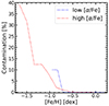 |
Fig. A.1. Running average of halo contamination in the disc in variable [Fe/H] bins with Vϕ > 110 Kms−1. The red dotted line represents high α and the blue dotted line represents low α. |
Appendix B: Age-Metallicity PDFs
Figure B.1 shows age-metallicity PDFs for 4 α-poor and metal-poor stars. The internal ID of each star according to the Gaia-ESO catalogue is provided in the title. The colour scale represents normalised probability density.
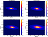 |
Fig. B.1. Age-metallicity PDFs for 4 α-poor and metal-poor stars. Each panel is a 2D histogram of the BeSPP posterior PDF in the [Fe/H]-Age projection with 1, 2, 3-σ contours. The colour scale displays the probability. |
All Tables
Sensitivity of the astrophysical parameters of the stellar sample to changes in the input data and in methodology (see text).
All Figures
|
Fig. 1. Photometry of the observed sample. Left panel shows the distribution in the Gaia magnitudes, G vs. GBP − GRP. Right panel shows the distribution in the VHS magnitudes, J vs. J − Ks (see Sect. 2). |
| In the text | |
|
Fig. 2. Spatial distribution of the observed sample. The vertical axis represents the height above the disc plane in kpc and the horizontal represents the Galactocentric radius in kpc. The colour scale shows normalised density from 0.07% (dark blue) to 100% (dark red). |
| In the text | |
|
Fig. 3. Distribution of the observed sample in the Teff − log g plane. The targets enclosed within the red box represent the sample used for the analysis of ages. |
| In the text | |
|
Fig. 4. Synthetic stellar population to simulate the selection effect of Gaia-ESO survey and of the observed stellar sample. Here, the results of the simulation at 1 kpc are shown for the blue box (top row) and red box (bottom row), as defined in Sect. 2. Right: completeness fraction, defined as the ratio of stars with cut to the number of stars without cut, that is, the larger the number the more stars are retained in the population after applying the colour cuts (Sect. 2). In case of no bias, the completeness fraction is unity 1. |
| In the text | |
|
Fig. 5. Densities of NLTE abundances of [Mg/Fe] as a function of [Fe/H]. The dashed lines represent the average [Mg/Fe] value for stars which are α-rich (red) and α-poor (blue). |
| In the text | |
|
Fig. 6. Phase-space of the observed Gaia-ESO sample: azimuthal velocity, Vϕ, versus radial velocity, Vr, coloured in density. The upper panels represent the α-poor population, and the lower panels represent the α-rich population. Each population is split into two [Fe/H] bins: metal-poor and metal solar-rich. The blue ellipse represents the halo distribution following the multi-Gaussian approach described in Belokurov et al. (2018) to determine halo contamination within the disc. |
| In the text | |
|
Fig. 7. Density distribution in actions Jr and Lz for our identified components. The black line in the lower panel represents the Solar Lz value of 1995 kpc km s−1. |
| In the text | |
|
Fig. 8. Number of stars (vertical axis) older than 9 Gyr with respect to the total number (annotated as text) of α-poor, rich stars (respectively) in a given [Fe/H] bin. Grey dotted lines represent [Fe/H] bin boundaries. Blue data represents α-poor stars, red data represents α-rich stars. The solid lines represent the left y-scale: fraction of stars with ages (τ) more than 9 Gyr, the dashed lines represent the right y-scale: fraction of stars with redshift (z) more than 2. |
| In the text | |
|
Fig. A.1. Running average of halo contamination in the disc in variable [Fe/H] bins with Vϕ > 110 Kms−1. The red dotted line represents high α and the blue dotted line represents low α. |
| In the text | |
|
Fig. B.1. Age-metallicity PDFs for 4 α-poor and metal-poor stars. Each panel is a 2D histogram of the BeSPP posterior PDF in the [Fe/H]-Age projection with 1, 2, 3-σ contours. The colour scale displays the probability. |
| In the text | |
Current usage metrics show cumulative count of Article Views (full-text article views including HTML views, PDF and ePub downloads, according to the available data) and Abstracts Views on Vision4Press platform.
Data correspond to usage on the plateform after 2015. The current usage metrics is available 48-96 hours after online publication and is updated daily on week days.
Initial download of the metrics may take a while.