| Issue |
A&A
Volume 682, February 2024
|
|
|---|---|---|
| Article Number | A22 | |
| Number of page(s) | 9 | |
| Section | Galactic structure, stellar clusters and populations | |
| DOI | https://doi.org/10.1051/0004-6361/202347569 | |
| Published online | 31 January 2024 | |
The most stringent upper limit set on the mass of a central black hole in 47 Tucanae using dynamical models
1
Dipartimento di Fisica e Astronomia “Augusto Righi”, Università di Bologna, Via Piero Gobetti 93/2, 40129 Bologna, Italy
2
INAF – Osservatorio di Astrofisica e Scienza dello Spazio di Bologna, Via Piero Gobetti 93/3, 40129 Bologna, Italy
e-mail: alessandro.dellacroce@inaf.it
3
INAF – Osservatorio astronomico di Padova, Vicolo Osservatorio 5, 35122 Padova, Italy
4
Dipartimento di Fisica e Astronomia, Università di Padova, Vicolo Osservatorio 3, 35122 Padova, Italy
5
Physics Departement, University of Pisa, Largo Bruno Pontecorvo, 3, 56127 Pisa, Italy
6
INFN, Largo B. Pontecorvo 3, 56127 Pisa, Italy
Received:
26
July
2023
Accepted:
21
October
2023
Globular clusters (GCs) have been proposed as promising sites for discovering intermediate-mass black holes (IMBHs), offering the possibility to gain crucial insights into the formation and evolution of these elusive objects. The Galactic GC 47 Tucanae (also known as NGC 104) has been suggested as a potential IMBH host, yet previous studies have yielded conflicting results. Therefore, we present a set of self-consistent dynamical models based on distribution functions (DFs) that depend on action integrals to assess the presence (or absence) of an IMBH in 47 Tucanae. Leveraging the state-of-the-art Multi Unit Spectroscopic Explorer (MUSE) and Hubble Space Telescope (HST) data, we analyzed the three-dimensional (3D) kinematics of the cluster’s central regions, fitting individual star velocities down to the sub-arcsec scale (approximately 10−2 pc). According to our analysis, the inner kinematics of 47 Tucanae is incompatible with a central BH more massive than 578 M⊙ (at 3σ). This is the most stringent upper limit placed thus far on the mass of a putative IMBH in 47 Tucanae via a dynamical study.
Key words: black hole physics / methods: statistical / techniques: radial velocities / proper motions / stars: kinematics and dynamics / globular clusters: individual: 47 Tucanae
© The Authors 2024
 Open Access article, published by EDP Sciences, under the terms of the Creative Commons Attribution License (https://creativecommons.org/licenses/by/4.0), which permits unrestricted use, distribution, and reproduction in any medium, provided the original work is properly cited.
This article is published in open access under the Subscribe to Open model. Subscribe to A&A to support open access publication.
1. Introduction
Intermediate-mass black holes (IMBHs) are classified as black holes (BHs) with masses in the range of 102 − 105 M⊙ (Greene et al. 2020), setting them between stellar-mass BHs and of supermassive BHs (SMBHs). The discovery of SMBHs at z = 7.5, when the Universe was only 0.7 Gyrs old (Bañados et al. 2018), poses a challenge to theories of SMBH formation (Volonteri 2010). Since IMBHs are thought to be the possible seeds from which SMBHs had grown at early times, finding evidence for IMBHs would provide insights into BH formation mechanisms. However, there has been no firm evidence presented for the existence of BHs in the range 102 − 105 M⊙ thus far (see e.g., den Brok et al. 2015; Nguyen et al. 2018; Abbott et al. 2020).
GCs are considered good candidates for hosting an IMBH because (i) theoretically they are expected to be promising sites for IMBH formation (Miller & Hamilton 2002; Portegies Zwart et al. 2004) and (ii) empirically central IMBHs are predicted in GCs as a natural extrapolation of the Magorrian et al. (1998) relation between central BH mass and bulge mass observed in galaxies. The presence of IMBHs in GCs has been investigated by means of different techniques, such as radio emission (e.g., Strader et al. 2012; Tremou et al. 2018), kinematic studies of the innermost stars (e.g., Gerssen et al. 2002; Vitral et al. 2023), and studies that constrain the gravitational field using the timing of radio pulsars (e.g., Kızıltan et al. 2017; Abbate et al. 2018).
The Galactic GC 47 Tucanae is arguably one of the best targets to look for an IMBH, mainly because of its high density and mass (Miller & Hamilton 2002; Portegies Zwart et al. 2004; Giersz et al. 2015). It is also relatively nearby (≃4.5 kpc), which allows for detailed studies of the central kinematics. Thus, it has been studied using different approaches to investigate the possible presence of an IMBH. Some studies carried out radio observations of the core of 47 Tucanae (e.g., de Rijcke et al. 2006; Tremou et al. 2018), finding no evidence of a significant emission. Tremou et al. (2018) placed a 3σ upper limit at M• < 1040 M⊙, while de Rijcke et al. (2006) found a broader limit of M• < 670 − 2060 M⊙, depending on different assumptions on the gas density, gas temperature, and the fraction of rest-mass energy of the infalling matter converted into radiation. Comparing spin-down measurements for 19 millisecond pulsars (MSPs) identified in 47 Tucanae, Kızıltan et al. (2017) found that an IMBH of mass  is required to reproduce the accelerations and the cumulative spatial distribution of MSPs. Hénault-Brunet et al. (2020) found that a total mass of
  in stellar-mass BHs could explain the stellar kinematics and spatial distribution (Hénault-Brunet et al. 2020, without IMBH). Exploiting a set of HST PM measurements of the central regions of 47 Tucanae, Mann et al. (2020) found that the stellar BH population cannot fully account for the observed velocity dispersion, even if a BH and neutron star retention fraction of the 100% is assumed. These authors concluded that an additional massive component with a mass M• = 808 − 4710 M⊙ (depending on the retention fraction) is favored.
The tension among some of the aforementioned results suggests that the question of the presence of an IMBH in 47 Tucanae requires further investigation. In this work, we address the problem by means of a stellar dynamical approach that combines state-of-the-art structural and kinematic data of 47 Tucanae with flexible self-consistent models of stellar systems which allow for the presence of a central IMBH.
2. Dynamical models
In this work, we use dynamical models based on DFs that depend on the action integrals J (see e.g. Arnold 1989; Binney & Tremaine 2008). Describing a stellar system as an ensemble of orbits, we can represent each orbit through its actions. Orbits with small |J| populate the internal regions of the clusters, whereas large |J| values describe orbits in the external regions (Binney & Tremaine 2008). This approach has a few important advantages: (i) the model is physical since the DF is always non-negative by construction; (ii) the velocity anisotropy, as well as any physical property of the system, are self-consistently computed directly from the DF (see Sect. 2.3); and (iii) the extension to multi-component systems, for instance galaxies with a stellar and dark matter component (Piffl et al. 2015; Binney & Piffl 2015; Pascale et al. 2018) or GCs with a central BH (Pascale et al. 2019), is straightforward.
2.1. Model for the stellar component
We consider models where the stellar component of 47 Tucanae is described by the following DF
![$$ \begin{aligned} f_\star (\boldsymbol{J}) =&f_0\,M_\star \,\left[ 1+\left(\frac{J_0}{h(\boldsymbol{J})} \right)^{\zeta }\right]^{\Gamma /\zeta } \times \left[ 1+\left(\frac{g(\boldsymbol{J})}{J_0} \right)^{\zeta }\right]^{-(B-\Gamma )/\zeta } \nonumber \\&\times \text{ exp}\,{\left[-\left(\frac{g(\boldsymbol{J})}{J_\text{cut}} \right)^{\alpha } \right]}\,, \end{aligned} $$](/articles/aa/full_html/2024/02/aa47569-23/aa47569-23-eq3.gif)
which produces models whose spatial distributions closely follow a double-power law model (Vasiliev 2019, but see also Evans & Williams 2014; Binney & Piffl 2015; Pascale et al. 2018, 2019) with an exponential cutoff in the system outskirts. Here, f0 is such that the DF is normalized to the total stellar mass M⋆ = (2π)3 ∫f⋆(J)d3J.
The dimensionless free parameters Γ and B primarily determine the inner (|J|≲J0) and outer (|J|≳J0) slopes in the action space, with J0 being the typical action at which this transition takes place. In the case of the double power-law model, Γ and B can be converted in the slopes of the three-dimensional (3D) density profile (Posti et al. 2015). The transition regime (|J|∼J0) is mainly regulated by ζ. Finally, the parameter α controls the sharpness of the exponential truncation for |J|≳Jcut, with Jcut (> J0) being the typical action value above which the exponential cutoff dominates the stellar distribution. The functions h(J) and g(J) are linear combinations of the actions defined as
where |L is the total angular momentum. These functions depend only on the two free parameters hz and gz, which mainly control the inner and outer anisotropy of the system, respectively (see Sect. 4.1 in Vasiliev 2019).
2.2. The gravitational potential
The total gravitational potential of the model cluster is the sum of the BH potential Φ• and the stellar potential Φ⋆. The BH potential is
where M• is the BH mass and r is the radial spherical coordinate. The stellar potential is determined by numerically solving (in an iterative fashion) the Poisson equation. At each iteration, i, the stellar potential is updated according to
![$$ \begin{aligned} \nabla ^2 \Phi _{\star ,\,i+1}&= 4\pi G \,\rho _{\star ,\,i} \nonumber \\&= 4\pi G \int d^3\boldsymbol{v}\, f_\star (\boldsymbol{J}[\boldsymbol{x},\boldsymbol{v}|\Phi _{\star ,\,i} + \Phi _\bullet ])\,, \end{aligned} $$](/articles/aa/full_html/2024/02/aa47569-23/aa47569-23-eq6.gif)
where ρ⋆ = ∫d3v f⋆(J) is the 3D stellar density and we have made explicit the dependence of the conversion between actions and Cartesian phase-space coordinates (x, v) on the total potential Φ⋆, i + Φ•. This shows that, given a DF, the stellar density distribution, as well as any physical property derived for the visible component (see Sect. 2.3), depends on the combination of stellar and BH potential. As an initial guess on Φ⋆, we adopted the isochrone potential (Binney & Tremaine 2008), but we note that the final stellar potential does not depend on this specific choice (see Vasiliev 2019).
Since the BH potential is spherically symmetric, and the h(J) and g(J) functions are defined such that the DF depends only on the radial action and the angular momentum modulus, the overall system is also spherical. Any integral of the DF that involves conversion between actions and Cartesian phase-space coordinates was performed with the AGAMA1 library (Vasiliev 2019).
2.3. Observable properties from a DF
Given a DF, we can calculate the observable properties of the model based on suitable integrations of the DF that allow us to compare theoretical models against the observations. Throughout this work, the DF is normalized to the total system mass (see Eq. (1)). The mass surface density distribution is then obtained via
where z is the line-of-sight (LOS) direction and R2 = r2 − z2 is the distance from the GC center on the plane of the sky. The stellar number density, n⋆, is then simply defined by the relation Σ⋆ ≡ m n⋆, where m is a nuisance parameter of the model with the dimension of a mass.
Furthermore, we can calculate projected velocity distributions as
where v3D = {vR, vT, vLOS} is the vector of 3D projected velocities (i.e., vR and vT on the plane of the sky, while vLOS is the LOS component). Since for the majority of the stars the 3D velocity is not available, it is useful to define the marginalized velocity distributions. In particular, the LOS velocity distribution
and the distribution in the plane-of-the-sky velocity components
such that they are normalized to unity in the velocity space. Finally, the velocity dispersion profile of the i-th velocity component (with i=“R”, “T” or “LOS”) is computed as
Equations (5)–(9) allow us to test our theoretical predictions against the data (see Sect. 3).
3. Data analysis
The family of dynamical models presented in Sect. 2 has eleven free parameters: the total stellar and BH masses, M⋆, and M•; the scale actions, J0, and Jcut; the dimensionless free parameters, ζ, Γ, B, gz, hz, and α; and the nuisance parameter, m. We explored this parameter space by comparing the models with a set of observables in a fully Bayesian framework. Details on the likelihood and the Markov chain Monte Carlo method used to explore the model posterior and calculate uncertainties on the free parameters (and on any derived quantity) are given in Appendix A.
As kinematic dataset, we used a combination of individual LOS velocities from Kamann et al. (2018, obtained using the MUSE spectrograph) and PMs from Libralato et al. (2022, derived from multi-epoch observations with HST).
Kamann et al. (2018) obtained individual LOS velocities using the MUSE spectrograph. This sample represents the largest compilation of LOS velocities covering the central regions of 47 Tucanae (up to 100″ from the GC center), with a typical velocity accuracy of 1 − 2 km s−1. To clean the sample of any possible contamination from binary systems, we selected only those stars with a probability of being an unresolved binary smaller than 50%, according to the criterion defined by Kamann et al. (2018). We also subtracted the average LOS velocity of the sample ( km s−1) from individual velocities. The final sample of LOS velocities used in this work thus comprises 14 601 stars.
Similarly, the catalog of PM data from Libralato et al. (2022) represents the most complete, homogeneous collection of PMs of stars in the cores of stellar clusters to date. To select stars with reliable PM estimates, we applied the quality selections described in Libralato et al. (2022, see their Sect. 4), retaining 68 954 stars. Moreover, we cleaned the sample of contaminants of the Small Magellanic Cloud by taking advantage of its high velocity (μα* = −4.716 ± 0.035 mas yr−1 and μδ = 1.325 ± 0.021 mas yr−1, Anderson & King 2003) relative to 47 Tucanae in the proper motion space. We thus removed all the stars further than 2.6 mas yr−1 from the cluster bulk velocity, corresponding to more than 50 km s−1 (i.e., larger than the central escape speed; Baumgardt & Hilker 2018).
Finally, we used the number density profile provided by de Boer et al. (2019) to model the stellar density distribution of the GC. These authors combined Gaia DR2 data in the external regions (projected distances from the center larger than ∼20′), with ground-based and HST observations from Trager et al. (1995) and Miocchi et al. (2013), respectively.
The dataset covers the whole cluster extent, from ∼1″ to the cluster outskirts. In the fitting procedure, we adopted a fixed background level of 0.08 stars arcmin−2 (see e.g., Hénault-Brunet et al. 2020).
In particular, we fit individual stellar velocities within 12″ from the center. This distance would correspond to the radius of influence, defined by the implicit relation  (where σLOS = σLOS(R) is the LOS velocity dispersion, see Eq. (9)) of a putative IMBH with mass M• = 104 M⊙. This is well above all previous claimed detections (Kızıltan et al. 2017; Mann et al. 2020) and the upper limits (McLaughlin et al. 2006). Our final kinematic sample consists of 260 stars, with either PM or LOS velocity, and 21 stars with the full 3D velocity. Beyond 12″, we used the velocity dispersion profiles computed using the same datasets.
Throughout the analysis, we adopted the center reported by Goldsbury et al. (2010) and the kinematic distance of 4.34 kpc (Libralato et al. 2022), without accounting for its 0.06 kpc error. The propagation of this error on PMs would contribute at 1% level, which is negligible compared to typical relative uncertainties on PM data around 16%.
Our models are non-rotating, though there is evidence that 47 Tucanae does rotate (Anderson & King 2003; Bellini et al. 2017; Kamann et al. 2018). However, Kamann et al. (2018) derived the dispersion profiles we used accounting for a rotationally dependent mean velocity, and rotation is erased when deriving PMs due to local corrections. A residual differential rotation could be present in the LOS sample of central stars (i.e., within 12″). However, in the very central regions, the LOS rotation velocity is expected to be ≃1 km s−1, which is a small fraction of the central LOS velocity dispersion (Kamann et al. 2018). We note that any residual rotation would likely bias the model toward higher IMBH masses, as it would increase the inferred central velocity dispersion.
4. Results
The left panel of Fig. 1 shows the posterior distribution of the IMBH mass. According to our analysis, we find no evidence of an IMBH in 47 Tucanae. Instead, we set an upper limit of M• < 578 M⊙ at the 3σ level. This is the most stringent upper limit on the mass of a putative central dark component in 47 Tucanae ever achieved by any dynamical study. The right panel of Fig. 1 shows the 3σ upper limit on the IMBH Rinfl, overplotted to the on-sky distribution of stars closer than 12″ to the center. It is clear that the kinematics of these stars put a very tight constraint on Rinfl, whose upper limit is comparable to the distance from the center of the innermost stars. We further verified this point, by performing additional fits where first the individual stars inside 12″, and then the velocity dispersion profiles were also removed. We found that the upper limit on the IMBH mass increases to a few thousand and to several hundred thousand solar masses, respectively.
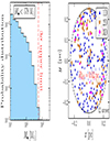 |
Fig. 1. Posterior distributions on the IMBH mass and region of influence in 47 Tucanae. Left: posterior distribution on the BH mass (blue histogram). The vertical line indicates the upper limit on the BH mass (578 M⊙) containing 99.7% (3σ) of the posterior distribution. Right: spatial distribution of the kinematic sample of individual stars inside a circumference of radius of 12″ (black curve). Each star is color-coded according to the available kinematic information: LOS velocity (i.e., 1D velocity) in dark blue, proper motion (2D) in brown, and full kinematic information (proper motion and LOS velocity, i.e., 3D) in magenta. The blue shaded area indicates the region that would be influenced by a central BH with mass 578 M⊙ (our 3σ upper limit), which has a radius of influence Rinfl = 0.02 pc (red curve). |
Figure 2 shows the PM and LOS velocity distributions for stars within 12″ from the center. Overplotted to the observations, we show the median model, and the 68% and 99.7% credible intervals (CIs) for the corresponding velocity distributions. Each model was convolved with a Gaussian distribution with a standard deviation equal to the observational median error in each component and was integrated over the radial extent covered by the datasets. The model reproduces the observed velocity distributions out to the tails (Fig. 2). We emphasize though that we did not fit the binned histograms, whereas we used an individual-star approach fully exploiting the datasets (see Eq. (A.3)).
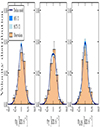 |
Fig. 2. Observed velocity distribution within 12″ from the cluster center, along the radial (left panel), tangential (central panel), and LOS (right panel) directions. The bars indicate uncertainties estimated as Poissonian errors on the bin counts. The median models (solid line), 68% (1σ), and 99.7% (3σ) CIs (shaded areas) are shown in blue (see text for details). |
The very good agreement between the model and the data can be further observed in Figs. 3 and 4, which show the projected velocity dispersion profiles and the stellar density profile, compared with the median and CIs of the corresponding theoretical profiles. We also compared (see Fig. 5) our model with measurements of the projected velocity anisotropy (data from Libralato et al. 2022), defined as σ⋆ T/σ⋆ R − 1, with σ⋆ R and σ⋆ T the radial and tangential velocity dispersion components, respectively (see Eq. (9)). Figure 5 shows that our model can reproduce the system velocity anisotropy remarkably well also compared to previous studies (see e.g., Dickson et al. 2023).
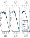 |
Fig. 3. Projected velocity dispersion profiles along the radial (left panel), tangential (central panel), and LOS (right panel) directions. Observations are shown as black points along with 1σ error bars. The blue line is the median model, while the shaded areas represent the 68% and the 99.7% CIs. |
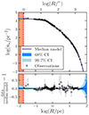 |
Fig. 4. Surface number density as a function of the projected distance from the cluster center. Observations are shown as black points (with 1σ error bars), whereas the model is shown in blue. The 68% and 99.7% CIs are also shown as shaded areas. The vertical dashed line represents the 3σ upper limit (0.02 pc) on the BH Rinfl. |
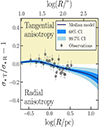 |
Fig. 5. Projected velocity anisotropy. Positive values of the anisotropy parameter correspond to tangential anisotropy, whereas negative ones to radial anisotropy. The median model is shown in blue and the corresponding CIs are shown as shaded areas. The black points are observational data from Libralato et al. (2022) with 1σ error bars. |
5. Comparisons with previous works
Our result is in tension with some previous studies claiming the presence of a massive IMBH in 47 Tucanae (see e.g., Kızıltan et al. 2017; Mann et al. 2020). In this section, we delve into the possible reasons for such discrepancies.
Kızıltan et al. (2017) used spin-down measurements for nineteen MSPs identified in 47 Tucanae. Comparing acceleration data with N-body simulations, they found evidence for a massive central BH with mass  . While a direct comparison with the study of Kızıltan et al. (2017) is not straightforward, as different dynamical models and data were used, we note that it is in general hard to perform a large exploration of possible initial conditions using N-body simulations. Dynamical models of equilibrium, on the other hand, allow us to perform a systematic exploration of the parameter space. In addition, in our model-data comparison, we fit simultaneously the spatial distribution and the full velocity distribution using individual stars, while Kızıltan et al. (2017) analyzed only those N-body simulations that better reproduced the density profile and the LOS velocity dispersion, which may not be representative of the full cluster kinematics.
However, as a further check, we verified whether our best-fit model is able to reproduce the measurements of MSPs. Figure 6 shows the cluster LOS acceleration data from the MSP sample (data from Ridolfi et al. 2016, and Freire et al. 2017) used by Kızıltan et al. (2017), as well as the maximum and minimum LOS acceleration allowed by our dynamical model. This quantity was computed as the maximum projection along the LOS of the radial acceleration, a(r), at any given projected distance from the center, R, namely,  . Interestingly, our model is compatible with all the upper limits and also with the central pulsars showing the highest accelerations (such as 47 Tuc-E, 47 Tuc-U, 47 Tuc-I, and 47 Tuc-S) without the need for an IMBH more massive than 578 M⊙ (at the 3σ level). The only outlier might be 47 Tuc-X, still compatible within 2σ with the median model.
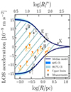 |
Fig. 6. LOS acceleration as a function of the projected distance from the center of 47 Tucanae. Black points are measurements, while orange ones are upper limits. Both were obtained from pulsars (data from Ridolfi et al. 2016; Freire et al. 2017). The label of each pulsar is shown either in orange or black. The blue line shows the maximum (if positive) and minimum (if negative) LOS acceleration allowed by our dynamical model at a given distance from the center. Similarly, the 68% and 99.7% CIs on the maximum and minimum LOS acceleration are shown as shaded areas. The hatched area is the allowed LOS acceleration space. |
Using dynamical models based on the Jeans equations coupled with PM data of the cluster center from HST, Mann et al. (2020) found that a massive IMBH with mass 808 − 4610 M⊙ is required to explain the central kinematics. While employing the same dataset would be the best approach to understand the possible reasons that lead to a discrepancy, we note that the work of Mann et al. (2020) focused on reproducing the system velocity dispersion. On the contrary, our DF-based models and individual-star approach (see Appendix A) make the most of the kinematic sample, since it does not condense the kinematic information into few radial bins. Instead, our approach is to model, in a continuous way, the full shape of the cluster’s velocity distribution in the center. This approach provides more stringent constraints on the presence of a putative massive dark component in the center (see Pascale et al. 2019). Furthermore, we also used LOS data to probe the 3D kinematics.
Finally, we note that our result is consistent with the findings of McLaughlin et al. (2006) and Hénault-Brunet et al. (2020). Using HST data and Jeans modeling, McLaughlin et al. (2006) put an upper limit of about 1578 M⊙ at the 1σ level, compatible with the much more stringent upper limit set by this study (578 M⊙ at 3σ). Moreover, Hénault-Brunet et al. (2020) constrained the overall mass budget in dark remnants (stellar-mass BH, neutron stars, and white dwarfs) possibly harbored at the center of 47 Tucanae. The upper limit set by the current work is consistent with the mass budget of  M⊙ found by Hénault-Brunet et al. (2020). Although our analysis only considers a point-like central mass, such as an IMBH, the upper limit on the central mass we have found would also apply to an extended spherical central object.
6. Conclusions
In this work, we address the problem of the presence of a putative IMBH at the center of the GC 47 Tucanae, using dynamical models based on DFs depending on the action integrals. We modeled state-of-the-art data providing information on the spatial distribution, along with both the LOS and on-sky kinematics up to the very central regions of the cluster. Also, we employed a star-by-star approach in the central region to fully exploit the data and model the full shape of the velocity distribution. According to our analysis, we ruled out (at the 3σ level) the presence of a dark central component more massive than 578 M⊙. To date, this is the most stringent upper limit that has been set in 47 Tucanae by any dynamical study. While this result is consistent with other studies (e.g., McLaughlin et al. 2006; Hénault-Brunet et al. 2020), it is in tension with those studies claiming the detection of an IMBH in 47 Tucanae (see e.g., Mann et al. 2020; Kızıltan et al. 2017). Despite the very stringent upper limit we set in this study, more sophisticated dynamical models and novel data with greater precision would shed further light on the nature of a putative central dark component in 47 Tucanae, as well as in other GCs. For instance, multi-mass modeling would allow us to account for stellar evolution and mass segregation (Gieles & Zocchi 2015).
From the point of view of the data, more extensive coverage of the central regions and progressively better-defined cluster centers and distances would certainly provide more robust results. Future facilities, such as the Extremely Large Telescope, will measure the stellar kinematics of GC centers with unprecedented accuracy, likely providing new and exciting data for this area of research.
Finally, we note that the methodology presented in this work could be applied to any GC in our Galaxy, regardless of the particular data available, whether pertaining to either PMs or LOS velocities only or full 3D kinematic information, as done in the present study. In addition, this approach is not limited to GCs and could be also used to explore the presence of central BHs in external galaxies (Pascale et al., in prep.).
Acknowledgments
We thank the anonymous referee for their comments. We are grateful to Sebastian Kamann for providing us with the MUSE data and to Andrea Bellini for fruitful discussions.
References
- Abbate, F., Possenti, A., Ridolfi, A., et al. 2018, MNRAS, 481, 627 [NASA ADS] [CrossRef] [Google Scholar]
- Abbott, R., Abbott, T. D., Abraham, S., et al. 2020, Phys. Rev. Lett., 125, 101102 [Google Scholar]
- Anderson, J., & King, I. R. 2003, AJ, 126, 772 [NASA ADS] [CrossRef] [Google Scholar]
- Arnold, V. 1989, Mathematical Methods of Classical Mechanics (Springer), 60 [CrossRef] [Google Scholar]
- Bañados, E., Venemans, B. P., Mazzucchelli, C., et al. 2018, Nature, 553, 473 [Google Scholar]
- Baumgardt, H., & Hilker, M. 2018, MNRAS, 478, 1520 [Google Scholar]
- Bellini, A., Bianchini, P., Varri, A. L., et al. 2017, ApJ, 844, 167 [NASA ADS] [CrossRef] [Google Scholar]
- Binney, J., & Piffl, T. 2015, MNRAS, 454, 3653 [NASA ADS] [CrossRef] [Google Scholar]
- Binney, J., & Tremaine, S. 2008, Galactic Dynamics, 2nd edn. (Princeton, NJ: Princeton University Press) [Google Scholar]
- de Boer, T. J. L., Gieles, M., Balbinot, E., et al. 2019, MNRAS, 485, 4906 [Google Scholar]
- den Brok, M., Seth, A. C., Barth, A. J., et al. 2015, ApJ, 809, 101 [NASA ADS] [CrossRef] [Google Scholar]
- de Rijcke, S., Buyle, P., & Dejonghe, H. 2006, MNRAS, 368, L43 [NASA ADS] [CrossRef] [Google Scholar]
- Dickson, N., Hénault-Brunet, V., Baumgardt, H., Gieles, M., & Smith, P. J. 2023, MNRAS, 522, 5320 [NASA ADS] [CrossRef] [Google Scholar]
- Evans, N. W., & Williams, A. A. 2014, MNRAS, 443, 791 [NASA ADS] [CrossRef] [Google Scholar]
- Foreman-Mackey, D., Hogg, D. W., Lang, D., & Goodman, J. 2013, PASP, 125, 306 [Google Scholar]
- Freire, P. C. C., Ridolfi, A., Kramer, M., et al. 2017, MNRAS, 471, 857 [Google Scholar]
- Gerssen, J., van der Marel, R. P., Gebhardt, K., et al. 2002, AJ, 124, 3270 [NASA ADS] [CrossRef] [Google Scholar]
- Gieles, M., & Zocchi, A. 2015, MNRAS, 454, 576 [NASA ADS] [CrossRef] [Google Scholar]
- Giersz, M., Leigh, N., Hypki, A., Lützgendorf, N., & Askar, A. 2015, MNRAS, 454, 3150 [Google Scholar]
- Goldsbury, R., Richer, H. B., Anderson, J., et al. 2010, AJ, 140, 1830 [NASA ADS] [CrossRef] [Google Scholar]
- Greene, J. E., Strader, J., & Ho, L. C. 2020, ARA&A, 58, 257 [Google Scholar]
- Hénault-Brunet, V., Gieles, M., Strader, J., et al. 2020, MNRAS, 491, 113 [CrossRef] [Google Scholar]
- Kamann, S., Husser, T. O., Dreizler, S., et al. 2018, MNRAS, 473, 5591 [NASA ADS] [CrossRef] [Google Scholar]
- Kızıltan, B., Baumgardt, H., & Loeb, A. 2017, Nature, 542, 203 [Google Scholar]
- Libralato, M., Bellini, A., Vesperini, E., et al. 2022, ApJ, 934, 150 [NASA ADS] [CrossRef] [Google Scholar]
- Magorrian, J., Tremaine, S., Richstone, D., et al. 1998, AJ, 115, 2285 [Google Scholar]
- Mann, C. R., Richer, H., Heyl, J., et al. 2020, ApJ, 893, 86 [NASA ADS] [CrossRef] [Google Scholar]
- McLaughlin, D. E., Anderson, J., Meylan, G., et al. 2006, ApJS, 166, 249 [NASA ADS] [CrossRef] [Google Scholar]
- Miller, M. C., & Hamilton, D. P. 2002, MNRAS, 330, 232 [Google Scholar]
- Miocchi, P., Lanzoni, B., Ferraro, F. R., et al. 2013, ApJ, 774, 151 [Google Scholar]
- Nelson, B., Ford, E. B., & Payne, M. J. 2014, ApJS, 210, 11 [Google Scholar]
- Nguyen, D. D., Seth, A. C., Neumayer, N., et al. 2018, ApJ, 858, 118 [NASA ADS] [CrossRef] [Google Scholar]
- Pascale, R., Posti, L., Nipoti, C., & Binney, J. 2018, MNRAS, 480, 927 [Google Scholar]
- Pascale, R., Binney, J., Nipoti, C., & Posti, L. 2019, MNRAS, 488, 2423 [NASA ADS] [CrossRef] [Google Scholar]
- Piffl, T., Penoyre, Z., & Binney, J. 2015, MNRAS, 451, 639 [NASA ADS] [CrossRef] [Google Scholar]
- Portegies Zwart, S. F., Baumgardt, H., Hut, P., Makino, J., & McMillan, S. L. W. 2004, Nature, 428, 724 [Google Scholar]
- Posti, L., Binney, J., Nipoti, C., & Ciotti, L. 2015, MNRAS, 447, 3060 [Google Scholar]
- Ridolfi, A., Freire, P. C. C., Torne, P., et al. 2016, MNRAS, 462, 2918 [Google Scholar]
- Strader, J., Chomiuk, L., Maccarone, T. J., et al. 2012, ApJ, 750, L27 [NASA ADS] [CrossRef] [Google Scholar]
- Ter Braak, C., & Vrugt, J. 2008, Stat. Comput., 18, 435 [CrossRef] [Google Scholar]
- Trager, S. C., King, I. R., & Djorgovski, S. 1995, AJ, 109, 218 [NASA ADS] [CrossRef] [Google Scholar]
- Tremou, E., Strader, J., Chomiuk, L., et al. 2018, ApJ, 862, 16 [Google Scholar]
- Vasiliev, E. 2019, MNRAS, 482, 1525 [Google Scholar]
- Vitral, E., Libralato, M., Kremer, K., et al. 2023, MNRAS, 522, 5740 [CrossRef] [Google Scholar]
- Volonteri, M. 2010, A&ARv, 18, 279 [Google Scholar]
Appendix A: Model and data comparison
We inferred the model’s free parameters in a Bayesian framework. In particular, this was done by defining the vector of 11 free parameters θ ≡ {log M⋆, log J0, ζ, Γ, B, gz, hz, log Jcut, α, log M•, m}, namely the nine DF parameters (see Eq. 1), the logarithm of the IMBH mass (log M•), and the normalization factor of the density profile (m). Thus, we can express the posterior distribution as

where D is the data vector, including both the kinematic sample and the surface density profile. The p(θ) and p(D|θ)≡ℒ(D) terms on the right-hand side of the equation are, respectively, the prior on the free parameters and the likelihood.
Assuming that all the data sets are independent of each other, we decompose the logarithm of the likelihood into the sum of the different terms

We stress that for the cluster central region, we adopt a star-by-star approach modeling the velocity and error of each of the Nstars stars. The resulting likelihood is
where ℱ ≡ 𝒱 * 𝒩. Therefore, for each star j, the velocity distribution (𝒱, see Eqs. 6 through 8, computed at the observed projected distance, Rj) is convolved (*) with observational errors, represented by a zero-mean, multivariate Gaussian (𝒩). The Gaussian covariance matrix has diagonal elements equal to the errors squared,  , and zero off-diagonal terms. The resulting function is evaluated at the observed velocity (vj). When the full kinematic information (PM and LOS velocity) is not available for the j-th star, we marginalize over the missing velocity components (see Eqs. 7, and 8).
For the velocity dispersions outside the central 12", we define
with σi, k being the velocity dispersion of the i-th component in the k-th radial bin (centered in Rk), δσi, k the corresponding error, and σ⋆ i(Rk) the model prediction. Also, Nbin, i is the total number of bins in which the velocity dispersion was obtained. Similarly, for the density profile, we have
where nl, δnl, and Nprof are the observed number density, the corresponding error, and the number of bins of the surface density profile, respectively.
All the physical quantities of the model are self-consistently computed from the DF (see Section 2.3). For all the parameters, we assumed uniform priors (Table A.1 for the specific prior ranges adopted). In particular, for the IMBH mass, we adopted a lower limit of 10 M⊙, well below the nominal definition of IMBH. Also, a less massive BH would have Rinfl < 10−3 pc, with a negligible impact on observables. We explored the free-parameter space by means of a Markov chain Monte Carlo algorithm (MCMC), using the emcee Python package (Foreman-Mackey et al. 2013). The algorithm was run with 112 walkers for about 7000 steps each. We used a mixture of moves developed by Ter Braak & Vrugt (2008), and Nelson et al. (2014) to achieve a more efficient exploration of the parameter space. For each walker, we discarded the first 2500 steps to account for the initial convergence phase, while exploring the prior. Afterward, we accounted for the correlation between subsequent samples, taking one sample every 100. Finally, we obtained about 5000 independent posterior samples. In Fig. A.1, we show the corner plot with both the marginalized posterior distributions (diagonal panels) and 2D joint distributions (lower-diagonal panels).
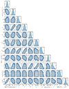 |
Fig. A.1. 1D (diagonal panels) and 2D (lower-diagonal panels) marginalized, posterior distributions over the model’s free parameters. See Section 2 for a description of the parameters. Prior ranges, median values, 68%, and 99.7% CIs for each parameter are reported in Table A.1. |
Free parameters of the model.
In Table A.1, we list the parameter prior ranges and the posterior values from the MCMC fitting. For each model free parameter, we report the median value, as well as the 68% (1σ) and 99.7% (3σ) CIs, computed from posterior samples. We note that all the free parameters are well constrained within the prior ranges. This indicates that the adopted intervals were well suited for a thorough exploration of the free-parameters space and there is no evidence for any need to extend these ranges.
All Tables
All Figures
|
Fig. 1. Posterior distributions on the IMBH mass and region of influence in 47 Tucanae. Left: posterior distribution on the BH mass (blue histogram). The vertical line indicates the upper limit on the BH mass (578 M⊙) containing 99.7% (3σ) of the posterior distribution. Right: spatial distribution of the kinematic sample of individual stars inside a circumference of radius of 12″ (black curve). Each star is color-coded according to the available kinematic information: LOS velocity (i.e., 1D velocity) in dark blue, proper motion (2D) in brown, and full kinematic information (proper motion and LOS velocity, i.e., 3D) in magenta. The blue shaded area indicates the region that would be influenced by a central BH with mass 578 M⊙ (our 3σ upper limit), which has a radius of influence Rinfl = 0.02 pc (red curve). |
| In the text | |
|
Fig. 2. Observed velocity distribution within 12″ from the cluster center, along the radial (left panel), tangential (central panel), and LOS (right panel) directions. The bars indicate uncertainties estimated as Poissonian errors on the bin counts. The median models (solid line), 68% (1σ), and 99.7% (3σ) CIs (shaded areas) are shown in blue (see text for details). |
| In the text | |
|
Fig. 3. Projected velocity dispersion profiles along the radial (left panel), tangential (central panel), and LOS (right panel) directions. Observations are shown as black points along with 1σ error bars. The blue line is the median model, while the shaded areas represent the 68% and the 99.7% CIs. |
| In the text | |
|
Fig. 4. Surface number density as a function of the projected distance from the cluster center. Observations are shown as black points (with 1σ error bars), whereas the model is shown in blue. The 68% and 99.7% CIs are also shown as shaded areas. The vertical dashed line represents the 3σ upper limit (0.02 pc) on the BH Rinfl. |
| In the text | |
|
Fig. 5. Projected velocity anisotropy. Positive values of the anisotropy parameter correspond to tangential anisotropy, whereas negative ones to radial anisotropy. The median model is shown in blue and the corresponding CIs are shown as shaded areas. The black points are observational data from Libralato et al. (2022) with 1σ error bars. |
| In the text | |
|
Fig. 6. LOS acceleration as a function of the projected distance from the center of 47 Tucanae. Black points are measurements, while orange ones are upper limits. Both were obtained from pulsars (data from Ridolfi et al. 2016; Freire et al. 2017). The label of each pulsar is shown either in orange or black. The blue line shows the maximum (if positive) and minimum (if negative) LOS acceleration allowed by our dynamical model at a given distance from the center. Similarly, the 68% and 99.7% CIs on the maximum and minimum LOS acceleration are shown as shaded areas. The hatched area is the allowed LOS acceleration space. |
| In the text | |
|
Fig. A.1. 1D (diagonal panels) and 2D (lower-diagonal panels) marginalized, posterior distributions over the model’s free parameters. See Section 2 for a description of the parameters. Prior ranges, median values, 68%, and 99.7% CIs for each parameter are reported in Table A.1. |
| In the text | |
Current usage metrics show cumulative count of Article Views (full-text article views including HTML views, PDF and ePub downloads, according to the available data) and Abstracts Views on Vision4Press platform.
Data correspond to usage on the plateform after 2015. The current usage metrics is available 48-96 hours after online publication and is updated daily on week days.
Initial download of the metrics may take a while.