| Issue |
A&A
Volume 682, February 2024
|
|
|---|---|---|
| Article Number | A56 | |
| Number of page(s) | 16 | |
| Section | Interstellar and circumstellar matter | |
| DOI | https://doi.org/10.1051/0004-6361/202244628 | |
| Published online | 01 February 2024 | |
Exploring the dust grain size and polarization mechanism in the hot and massive Class 0 disk IRAS 16293-2422 B★
1
Max-Planck-Institut für extraterrestrische Physik,
Gießenbachstraße 1,
85748
Garching bei München,
Germany
e-mail: This email address is being protected from spambots. You need JavaScript enabled to view it.
2
Department of Physics, National Sun Yat-Sen University,
No. 70, Lien-Hai Road,
Kaohsiung City
80424,
Taiwan,
ROC
3
Department of Astronomy, The University of Texas at Austin,
2500 Speedway,
Austin,
TX
78712,
USA
4
Department of Astronomy, University of Arizona,
933 N. Cherry Ave.,
Tucson,
AZ
85721,
USA
Received:
29
July
2023
Accepted:
1
November
2023
Abstract
Context. Multiwavelength dust continuum and polarization observations arising from self-scattering have been used to investigate grain sizes in young disks. However, the likelihood of self-scattering being the polarization mechanism in embedded disks decreases for very highly optically thick disks and makes us reconsider some of the size constraints from polarization, particularly for younger and more massive disks. The 1.3 mm polarized emission detected toward the hot (≳400 K) Class 0 disk IRAS 16293-2422 B has been attributed to self-scattering, with predictions of bare grain sizes between 200 and 2000 µm.
Aims. We aim to investigate the effects of changing the maximum grain sizes in the resultant continuum and continuum polarization fractions from self-scattering for a hot and massive Class 0 disk extracted from numerical simulations of prestellar core collapse and to compare them with IRAS 16293 B observations.
Methods. We compared new and archival dust continuum and polarization observations at high resolution between 1.3 and 18 mm to a set of synthetic models. We developed a new publicly available tool to automate this process called Synthesizer. This tool is an easy-to-use program for generating synthetic observations from numerical simulations.
Results. Optical depths are in the range of 130 to 2 from 1.3 to 18 mm, respectively. Predictions of significant grain growth populations, including amax = 1000 µm, are comparable to the observations from IRAS 16293 B at all observed wavelengths. The polarization fraction produced by self-scattering reaches a maximum of approximately 0.1% at 1.3 mm for a maximum grain size of 100 µm, which is an order of magnitude lower than the grain size observed toward IRAS 16293 B.
Conclusions. From comparison of the Stokes I fluxes, we conclude that significant grain growth could be present in the young Class 0 disk IRAS 16293 B, particularly in the inner hot region (< 10 au, T > 300 K) where refractory organics evaporate. The polarization produced by self-scattering in our model is not high enough to explain the observations at 1.3 and 7 mm, and such effects as dichroic extinction and polarization reversal of elongated aligned grains remain other possible but untested scenarios.
Key words: polarization / radiative transfer / scattering / protoplanetary disks / stars: protostars
Final reduced data are available at the CDS via anonymous ftp to cdsarc.cds.unistra.fr (130.79.128.5) or via https://cdsarc.cds.unistra.fr/viz-bin/cat/J/A+A/682/A56
NSF Astronomy and Astrophysics Postdoctoral Fellow.
© The Authors 2024
 Open Access article, published by EDP Sciences, under the terms of the Creative Commons Attribution License (https://creativecommons.org/licenses/by/4.0), which permits unrestricted use, distribution, and reproduction in any medium, provided the original work is properly cited.
This article is published in open access under the Subscribe to Open model.
Open Access funding provided by Max Planck Society.
1 Introduction
Circumstellar disks, which are the sites of planet formation, are relatively well studied in the more evolved Class II stage. However, in the earliest Class 0 phase, protostellar disks have only recently begun to be studied in detail (e.g., Maury et al. 2019; Segura-Cox et al. 2018; Tychoniec et al. 2020; Zamponi et al. 2021; Xu & Kunz 2021a,b; Xu 2022; Xu et al. 2023), and many of their properties, such as mass, temperature, and dust properties, remain unknown or highly debated. Since Class 0 protostellar disks set the initial conditions for planet formation, which could already be underway in the Class I phase (Sheehan & Eisner 2018; Segura-Cox et al. 2020; Michel et al. 2023), constraining the sizes of dust grains in disks at the earliest time possible is critical. This is usually done by constraining the variations of the spectral index at millimeter wavelengths, which can be related to the dust opacity index (Testi et al. 2014). In addition, polarization observations have proven to be a useful independent method to constrain the grain sizes in disks. These can be performed if the origin of the polarized emission is self-scattering (Lazarian & Hoang 2007a,b; Kataoka et al. 2015; Andersson et al. 2015; Tazaki et al. 2017). Self-scattering refers to the polarization of the dust thermal emission being scattered by the dust itself, and it produces emission polarized to a few percent at millimeter wavelengths for grain sizes in the micro- and millimeter range (Kataoka et al. 2017). The amount of polarization depends on the level of anisotropy of the radiation field generated by the self-scattered photons of the dust emission, which in turn depends on the inclination of the disk and the size of the scattering dust particles (Yang et al. 2016). The relation between the size of the dust grains and the maximum polarization fraction turns this polarized emission into a tool to estimate the level of grain growth at different evolutionary stages.
In the more evolved (Class II) protoplanetary disks, optical and near-infrared observations of scattered flux usually trace the emission from small dust grains that scatter off the protostellar flux in the upper layers of the disk (Avenhaus et al. 2018; Garufi et al. 2018, 2019, 2020). At millimeter wavelengths, the observed dust-scattered emission mainly originates from the dust thermal emission (Kataoka et al. 2015; Yang et al. 2016).
In this work, we explore the effect of changing the maximum grain sizes in the resultant continuum and polarization fractions by dust self-scattering at millimeter wavelengths. We use a model produced by a radiation-hydrodynamic (RHD) numerical simulation of core collapse. The disk formed is massive (~0.3 M⊙), hot (>300 K, within 10 au), and optically thick at millimeter wavelengths. This disk model successfully reproduces Stokes I fluxes from ALMA ~6–10 au resolution observations at 1.3 mm and 3 mm for the very young Class 0 disk IRAS 16293 B (Zamponi et al. 2021). Thus, we also aim to test whether we can reproduce the fluxes and levels of polarization fraction observed in this source when the polarization is produced by self-scattering of spherical grains in the Mie regime. We expand on our previous exploration of grain sizes in this young disk (Zamponi et al. 2021) by showing the effects of varying the maximum grain size (amax) in the model from 10 µm to 1000 µm. Furthermore, as the disk is hot enough to evaporate solid organics, we show the effects of evaporating water and potentially some organics within the so-called soot line and having grain growth within this region, as motivated by recent laboratory (Gundlach et al. 2018; Pillich et al. 2021) and observational (Liu et al. 2021) results.
IRAS 16293-2422 B is a well-studied Class 0 protostar located in the star-forming region ρ-Ophiuchi, and it is one of the closest and brightest protostars, at a distance of 141 pc (Dzib et al. 2018). The disk around the protostar is hot (Tb ≳ 400 K) and massive and likely subject to gravitational instabilities, as initially proposed by Rodríguez et al. (2005) and Dipierro et al. (2014) and recently confirmed by Zamponi et al. (2021). The source is very young (< 104 yr, Andre et al. 1993), and its water snowline extends over a 20 au radius (Zamponi et al. 2021), making it an ideal context to test the scenario proposed by recent laboratory experiments (Gundlach et al. 2018; Pillich et al. 2021; Li et al. 2021) that grain growth is boosted in dry conditions. The disk mass estimated by Zamponi et al. (2021) is 0.003 M⊙ in solid material, which would be 33 times higher than the minimum mass solar nebula of 30 M⊕ (in solids; Weidenschilling 1977; Andrews 2020). This implies that IRAS 16293B contains enough mass to form super-Earth planetesimals. Because of all these conditions, IRAS 16293B represents one of the ideal sites to probe grain growth at the earliest stages of star formation.
In younger Class 0 disks, although polarization by self-scattering at millimeter wavelengths has also been proposed (e.g., Cox et al. 2018; Sadavoy et al. 2018; Tsukamoto et al. 2022), studies simulating the feasibility of this mechanism in more realistic young disk models, such as 3D numerical simulations of disks formed out of the collapse of a core, have not been done. This is particularly important since the physical properties of deeply embedded disks appear different in numerical simulations (e.g., Zamponi et al. 2021; Xu & Kunz 2021a,b; Bate 2022) as compared to the widely used analytical models for Class II disks (Ballering & Eisner 2019).
In IRAS 16293-2422 B, polarized light was initially observed by Rao et al. (2009, 2014) with the SMA at 0.87 µm, who detected polarization fractions of around 1.4% distributed mostly azimuthally around the protostar location. The resolution of this detection was 0.6″ (85 au) and likely traced envelope scales, which correspond to the bridge structure connecting the northern and southern protostars (Jørgensen et al. 2016; Maureira etal. 2020). Additional observations were presented by Liu et al. (2018) with the VLA at 7 mm and a 1.5 times better resolution. These observations resolved down to 50 au and showed a similar polarization pattern and fraction (≲2%). More recently, a survey of 1.3 mm polarization observations toward Class 0 protostars in ρ-Ophiucus carried out by Sadavoy et al. (2019) at a two-times better resolution (0.2″; 30 au) found polarization signatures associated with self-scattering in inner regions of most of their sources. The polarization in the disk of IRAS 16293 B was found to be azimuthal, similar to the SMA and VLA observations; however, this pattern was associated the vector distribution to polarized self-scattering from an optically thick face-on disk, based on the models from Yang et al. (2017). The connection of a similar polarization pattern between 1.3 mm and 7 mm produced by self-scattering implies that grains can have sizes between 200 and 2000 µm. In this work, we use a disk model from numerical simulations to test this hypothesis.
This paper is structured as follows. In Sect. 2, we provide details on the archival and new observational data used in this work. In Sect. 3, we describe the dust model and polarization scheme used for the radiative transfer analysis. In Sect. 4, we present the results of the assessment of grains sizes through the Stokes I fluxes and our self-scattering models. In Sect. 5, we discuss grain growth and the possible mechanisms responsible for the observed polarization and other scenarios, and finally, in Sect. 6 we present the conclusions of this work.
2 Observations
2.1 ALMA and VLA archival data
We compiled archival multiwavelength polarization observations of IRAS 16293-2422 B at 1.3 mm (ALMA Band 6), 3 mm (ALMA Band 3), and 7 mm (JVLA Band Q). The 1.3 mm data used in this work are twofold. For the analysis presented in Sect. 4.1, we used high-resolution Stokes I continuum images with a resolution of 0.114″ × 0.069″ and a noise level of 104 µJy beam−1 (0.3 K; see colors cale in leftmost panel in Fig. 1). For the analysis of polarized data, we used publicly available Stokes I, Q, and U images by Sadavoy et al. (2018); each have a resolution of 0.18″ × 0.09″ and a noise level of 280 µJy beam−1 (0.4 K), 25 µJy beam−1 and 25 µJy beam−1, respectively. The Band 6 polarization vectors shown in Fig. 1 were masked in regions were the Stokes I flux is lower than 3σI and the polarized intensity is lower than 3σQ. The 3 mm data we used are only available in Stokes I, but it presents the highest resolution image of IRAS 16293 B currently available, with a beam size of 0.048″ × 0.046″ and a noise level of 17 µJy beam−1 (0.95 K). The data used at 7 mm contain full polarization information, with a resolution of 0.39″ × 0.24″ and a noise level of 35 µJy beam−1 (0.25 K). We masked polarization vectors following the same criteria as for Band 6 observations.
We refer the reader to Zamponi et al. (2021) for more information about the high-resolution ALMA observations at bands 6 and 3 as well as their calibration and imaging. Similarly, we refer to Liu et al. (2018) for the details on the observations, calibration, and imaging of the polarized data at the JVLA band Q.
2.2 VLA bands Ka and Ku observations
We present JVLA standard continuum mode observations at the Ka (9 mm) and Ku bands (18 mm) toward IRAS 16293-2422 B. Both are in the A array configuration. The Ka band observations were carried out on March 7, 2022 (project code: 22A-322, PI: Zamponi). The Ku band observations were carried out on January 2, 4, and 5, 2021 (project code: 20B-172, PI: Chia-Lin Ko). The pointing and phase referencing centers for our target source are RA = 16h32m22s.610 (J2000), Dec = -24°28′32″.61 (J2000) for our Ka band observations, and RA = 16h32m22s.620 (J2000), Dec = −24°28′32″.5 (J2000) for the Ku band. We employed the 3 bit sampler in both observations.
For the Ka band observations, 24 antennas were used with a projected baseline range of 794–34.4 km. The bandpass, phase, and amplitude calibrators used were J1256-0547, J1625-2527, and J1331+3030, respectively. We calibrated the data using the standard VLA Pipeline (v2021.2.0.128) and the Common Astronomy Software Applications (CASA; McMullin et al. 2007) package, release 6.2.1.7. The spectral configuration included ten narrow (16 MHz) and 52 wide (128 MHz) spectral windows. We created our continuum image using wide windows only, with a total bandwidth of 7 GHz centered at 33 GHz. We performed phase-only self-calibration iteratively in CASA. In each iteration, the cleaning was done with the deconvolver mtmfs, a robust parameter of 0.5, and scales of 0, 1, and 3 beams. The final image has a resolution of 0″.12×0″.05 (PA = −23.11°) and a noise level of 16µJy beam−1 (3 K).
For the Ku band observations, the absolute flux-passband and complex gain calibrators were 3C286 and J1625-2527. The projected baseline range is ~ 1.15–36.50 km. We manually followed the standard data calibration strategy using CASA (release 5.6.2). We utilized the built-in image model for 3C286 during the calibrations. After implementing the antenna position corrections, weather information, gain-elevation curve, and opacity model, we bootstrapped delay fitting and passband calibrations, and we then performed complex gain calibration. We applied the absolute flux reference to our complex gain solutions and then applied all the derived solution tables to the target source. Finally, we based our observations on 3C286 to solve the cross-hand delay and absolute polarization position angles and took J2355+4950 as a low polarization percentage calibrator when solving the leakage term (i.e., the D-term). We performed zeroth order (i.e., nterm=l) multifrequency synthesis imaging. The Briggs Robust=0 weighted image achieved a noise level of 47 µJy beam−1 and a 0″.23×0″.094 (PA = 5.2°) synthesized beam.
Finally, since all the observations shown in Fig. 1 have been taken at different times, we corrected the images for the proper motion of the source, which was calculated based on previous observations with the VLA (Hernández-Gómez et al. 2019) and the 3 mm observations presented here. The applied correction is RA: −11.8 ± 0.3 mas yr1 and Dec: −19.7 ± 1.3 mas yr1. We also aligned the observations to the observing time of the most recent Ka band observation (2022/03/07).
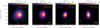 |
Fig. 1 IRAS 16293-2422 B observed at ALMA bands 6 and 3 and VLA bands Q, Ka, and Ku (from left to right). The cyan vectors represent polarization E-vectors (masked out below 3σI and 3σQ), and the scale bar indicates a 2% polarization fraction. The continuum data at 1.3 and 3 mm were presented by Zamponi et al. (2021), and the 1.3 mm polarization observations were presented by Sadavoy et al. (2018). The polarized continuum observations at 7 mm were obtained from Liu et al. (2018). The 9 mm and 18 mm continuum observations are presented for the first time by this work. The angular resolution of the observations are as follows: 0.114″ × 0.069″ at 1.3 mm (0.18″ × 0.09″ for polarized data); 0.048″ × 0.046″ at 3 mm; 0.39″ × 0.24″ at 7 mm; 0.12″ × 0.05″ at 9 mm; and 0.23″ × 0.09″ at 18 mm. |
3 Disk and dust model
3.1 Protostellar disk model
For comparison with the observations of the IRAS 16293-2422 B disk, we used a numerical simulation of the collapse of a prestellar core that results in a hot and gravitationally unstable protostellar disk. This simulation has been presented in Zamponi et al. (2021), and the resultant density and temperature structure is also shown in Fig. 2. In Zamponi et al. (2021), we showed that this disk can successfully reproduce both the 1.3 and 3 mm observed fluxes and the spectral index between both bands. This implies producing high brightness temperatures (e.g.,  at the peak) to match those from IRAS 16293B observed with ALMA. The disk was obtained from a simulation snapshot at a stage 18.2 kyr after the collapse of a 1 M⊙ spherical and isothermal cloud, simulated using the smoothed-particle-hydrodynamics (SPH) code sphNG (Bate et al. 1995). This simulation setup included a radiation transport scheme. This scheme helps more accurately reproduce the cooling and heating source terms along temporal evolution of the system and deliver more realistic gas temperature distributions. The mass in the disk at this point is ~0.3 M⊙. The gas temperature is ≳300 K within the central 10 au and decreases to ~200 K at the scales where two roughly symmetric spiral arms have formed (10–30 au; see Fig. 2).
To generate the radiative transfer model, we set the dust temperature equal to the gas temperature from the RHD simulation. This is justified because of the high densities found within the disk that allow the dust to be dynamically and thermally coupled with the gas (see also Zamponi et al. 2021). We assumed a homogeneous gas-to-dust density ratio of 100. We used the RADMC3D radiative transfer code (Dullemond et al. 2012) with a regular Cartesian grid generated by interpolating all particle positions. The particle interpolation and gridding was done with our newly developed tool, called Synthesizer (see Sect. 3.2), which automates the generation and execution of radiative transfer models from numerical simulations. The resulting dynamic range and spatial distribution of the gas density and temperature between our gridding scheme and that from Zamponi et al. (2021) are in very good agreement. The former gridding scheme used in Zamponi et al. (2021) consisted of a Voronoi tessellation of the particle locations, which was supported in POLARIS (Reissl et al. 2016), but this scheme is not yet fully supported in RADMC3D (beta feature).
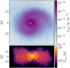 |
Fig. 2 Face-on gas density (top) and edge-on temperature (bottom) distributions across the midplane of the protostellar disk formed from the numerical simulations of the collapse of a core. We note that this is the disk we compared to the observations of IRAS 16293-2422 B. The white contour in the bottom panel represents the extension of the soot line at 300 K. This model is presented in greater detail in Zamponi et al. (2021). |
3.2 Synthesizer. From simulations to synthetic observations
To automate the comparison of observational data and simulation outputs, we developed a new tool called SYNTHESIZER, which we have made publicly available1 in the form of a Python package2. Synthesizer is a program to calculate synthetic images from either an analytical model or numerical simulations directly from the command line. For SPH simulations, it interpolates the particle positions into a rectangular Cartesian grid and then uses RADMC3D to perform a thermal Monte Carlo and ray tracing. Then it feeds the output image to CASA to generate a final synthetic observation. Support for polarization models, either by scattering or grain alignment, is also included. Additionally, the SYNTHESIZER includes a module called DUSTMIXER. This is a tool to generate dust opacity tables and full scattering matrices from the optical constants of a given material, all from the command line. DUSTMIXER also allows for the mixing of different materials and different grain sizes. Further information about this dust module can be found in Appendix A.
3.3 Grain sizes
In this work, we use a dust model similar to the one used by Zamponi et al. (2021), where spherical grains have a minimum size of 0.1 µm. This lower end of the size distribution was chosen based on the prediction for removal of very small grains during the stage of protostellar disk formation (Zhao et al. 2018; Silsbee et al. 2020). In this work, we explore maximum grain sizes in IRAS 16293B by showing the effect of amax on the resultant simulated fluxes. In Zamponi et al. (2021), we modeled the emission of IRAS 16293B using a dust population with amax = 10 µm only, which successfully reproduced the observed brightness temperatures. The millimeter scattering opacities in that case are negligible (see Fig. 3). The results in Zamponi et al. (2021) demonstrated that the low (<~2) 1.3–3 mm spectral index observed in the IRAS 16293 B disk could be reproduced without the need for larger grains in which the scattering opacities are important. The reason for this was that the resultant disk from the numerical simulation is both hot toward the inner layers and optically thick at millimeter wavelengths, and both are necessary conditions to recover the low observed alpha (see Fig. 9 in Zamponi et al. 2021). We extended the analysis by considering distributions with amax = 10, 100, and 1000 µm, and we compared the resulting images to the observations presented in Fig. (see Sect. 4.1).
The dust opacities computed for different models are presented in Fig. 3 (silicates + graphites and silicates + graphites + organics). The figure shows three panels, one for each maximum grain size tabulated in Table 1 for the four observing wavelengths from Fig. 1. For each amax, three different line styles represent absorption, scattering, and extinction opacities for a given composition (colored lines). When comparing the three panels of Fig. 3, one can see at a glance the relation between the albedo (κsca/κext) and the maximum grain size. The wavelength regime in which λ ~ 2πamax is also where the albedo is the highest. Because of this, the millimeter scattering opacities can vary by orders of magnitude for maximum grain sizes between 10 and 1000 µm. These differences are also reflected on the level of polarized scattered flux (produced by dust self-scattering) and turn them into a proxy of grain growth (Kataoka et al. 2016a,b; Yang et al. 2016; Stephens et al. 2017; Harris et al. 2018; Sadavoy et al. 2018; Ohashi et al. 2020; Lin et al. 2021).
3.4 Composition
Our fiducial dust mixture consisted of 62.5% astronomical silicates and 37.5% graphite (Sil:Gra curve in Fig. 3). The optical constants3 for the materials were obtained from Draine (2003a,b), respectively. However, carbon-bearing species in the interstellar medium may be present in many forms and shapes, and they may not all necessarily be crystallized as graphite. They can also be amorphous or ring-like (as in PAHs) carbonaceous. The predominant shape of carbonaceous material in space is hard to determine (Jager et al. 1998; Zubko et al. 2004; Birnstiel et al. 2018). According to Draine (2003a), molecules with sizes larger than 0.1 µm are likely to be crystallized. This is in fact the lower end of our size distribution (see Sect. 3.3); hence, we assumed graphite as a fiducial representation of the carbon budget in our dust model.
To consider the effects of carbon evaporation, we considered inclusions of refractory organics (Henning & Stognienko 1996) into the carbon mixture and studied the resulting differences in the overall opacity. Refractory organics have a considerably lower sublimation temperature (~300K, Jager et al. 1998; van’t Hoff et al. 2020; Li et al. 2021) compared to that of graphite (~2100 K). Taking into account the lower sublimation temperatures of certain carbonaceous materials is important because they decrease the dust mass in hot regions and result in an overall decrease in dust opacity. This sublimation zone within which the amount of carbon in the grains is reduced, also called the “soot line” (Kress et al. 2010; van’t Hoff et al. 2020), is likely to be present in IRAS 16293B at a radius of ~ 10 au based on the high (Tb > 400 K) brightness temperatures observed (see Fig. 1). The spatial extension of this region in the simulated disk is illustrated by the white contour in the edge-on temperature projection in Fig. 2, which extends radially up to ~10 au and vertically to ~8 au.
The difference between opacities with and without organics can be seen in Fig. 3. In the two compositions with carbon, the total carbon fraction of 37.5% is kept constant. For the one including refractory organics, we replaced 50% of the graphite by refractory organics, meaning both carbonaceous components have mass fractions of 18.75%. At millimeter wavelengths, the opacity of a dust population with amax of 10 or 100 µm is largely dominated by graphite instead of silicate. When we compared the two different compositions, that is, silicates-graphites versus silicates-graphites-organics, we observed that a mixture with inclusions of organics has a lower opacity than a purely graphitic material. This is because the opacity of pure graphite is larger than that of pure organics and including organics into the mixture implies a partial removal of graphite, since our carbon budget is maintained constant4. When considering evaporation of organics in our radiative transfer calculation, we changed the dust compositions accordingly. In regions where Tdust < 300 K, the dust is a mixture of silicates, graphites, and refractory organics, whereas in regions where Tdust ≥ 300 K (~ 10 au radius), we removed the organics from the mixture to mimic the sublimation of carbon and locally scaled down the dust-to-gas mass ratio by the corresponding mass-loss factor. Within the soot line, the organics get sublimated and removed from the dust grains. This produces a reduction in the dust mass and opacity that results in a reduction of the optical depth.
Two major features can be concluded from Fig. 3: (I) For every amax, the difference in opacity between both compositions is very small. (II) In the regime where λ ~ 2πamax, that is, where the albedo is at its maximum (Mie regime), the dust opacity is highly insensitive to variations in the dust composition. This means that observations of polarized emission produced by scattering can serve as a tool to constrain grain sizes but not compositions. The small differences we found for different compositions are associated with the resulting extinction opacity and not with the polarization pattern or fraction. We acknowledge that in some cases, variations in the scattering polarization patterns can indeed be produced by different dust compositions, as shown by Yang & Li (2020). Their works show that compositions like those from Kataoka et al. (2015) or Yang et al. (2016) can produce polarization reversal (i.e., 90-degree rotation of the vector angles) when elongated millimetric grains are present.
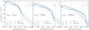 |
Fig. 3 Dust opacities for different maximum grain sizes and compositions. The three panels show, from left to right, dust opacities for a maximum grain size of 10, 100 & 1000 µm, respectively. Each panel contains opacities generated for a mixture of silicates and graphite (0.625–0.375) and a mixture of silicates, graphites and refractory organics (0.627–0.300–0.075; 80% of organics). The gray curve on every panel indicates the albedo of the fiducial composition (silicates and graphites). Four vertical gray lines indicate the observing wavelengths used in this study, corresponding to the observations from Fig. 1. The exact opacity values used in this work are listed in Table 1, for different amax and compositions, at all four wavelengths. |
Dust opacities (g cm−2) used in this work for different maximum grain sizes, for different compositions, and at four wavelengths.
3.5 Polarization by dust self-scattering
We performed radiative transfer calculations in all four Stokes components (I, Q, U, V) using the radiative transfer code RADMC3D (Dullemond et al. 2012) via the Synthesizer. To model the Stokes I fluxes produced, we ray traced the dust thermal emission along the line of sight and included the emission scattered by the dust grains; both are from stellar and dust thermal radiation. The dominant source of scattering at the millimeter wavelengths is the scattered dust thermal emission, namely, self-scattering (Kataoka et al. 2015).
The scattering of light in dusty media is commonly modeled as a stochastic process of absorption and re-emission of light (Bjorkman & Wood 2001) by means of a Monte Carlo simulation (Steinacker et al. 2013). The scattering event is modeled as the reemission of an absorbed photon in a new random direction. The likelihood for a given direction is not isotropically distributed but instead follows the commonly used phase function from Henyey & Greenstein (1941). However, this kind of scattering model considers only information about the light intensity and not of the polarization state (i.e., Stokes I only flux without Stokes Q and U). To calculate the polarized flux, the scattering process has to be represented by a matrix rotation of all four Stokes components. This process is also called full Mie scattering (Mie 1908; Bohren & Huffman 1983; Wolf & Voshchinnikov 2004) and is significantly more computationally expensive than the case concerning Stokes I only. To ensure both approaches (i.e., Stokes I only and full Mie) deliver similar Stokes I fluxes, we tested the convergence of the scattering Monte Carlo simulation. The convergence was reached at about 1010 photons.
The information associated with the linear polarization of light is stored in the Q and U components of the Stokes vector. We estimated the total linearly polarized intensity PI, polarization degree Pfrac, and polarization angle Pangle as
 (1)
(1)
 (2)
(2)
and
 (3)
(3)
respectively.
3.6 Synthetic observations
We post-processed the output from the radiative transfer with a series of synthetic observations using the observing setups of the ALMA and VLA observations shown in Fig. 1. This step was performed using the Synthesizer (see Sect. 3.2). Synthesizer uses the CASA (v5.6.2) software, and its SIMOBSERVE and TCLEAN tasks to produce a synthetic image from a model image created by the output of RADMC3D. The CASA scripts for the setup at every band are available within the Synthesizer public repository5.
All of the synthetic maps include the thermal noise associated with the corresponding observing setup (time, bandwidth, cycle, etc.) and lead to noise levels comparable to the real observations. In regions of the images where Q and U are not well detected, Eq. (1) leads to a positive bias in the polarized intensity that must be removed (Simmons & Stewart 1985; Vaillancourt 2006). The polarized intensity must then be debiased by taking into consideration the thermal noise in the polarization map σPI as
 (4)
(4)
where we assumed that σQ ~ σU ~ σPI (Vaillancourt 2006). When producing maps of polarized emission and polarization vectors from synthetic observations, we masked out the vectors at locations where I/σI < 3 and PI/σPI < 3, just as we did for the real observations in Fig. 1.
4 Results
4.1 Effects of different maximum grain sizes on the Stokes I fluxes
We started our analysis by producing synthetic observations of the Stokes I fluxes from the simulated disk at four different wavelengths, 1.3, 3, 9, and 18 mm, corresponding to the ALMA bands 6 and 3 and the VLA bands Ka and Ku (Fig. 1). All Stokes I images and profiles presented in this paper represent net fluxes. This means thermal plus scattered flux. For each band, we mimicked the observing setup of the real observations described in Sect. 2 and presented in Fig. 1. We extracted a cut of the brightness temperature maps along the east-west axis and plotted it as a function of physical offset from the peak, as shown in Fig. 4. All brightness temperature cuts were taken along the position of the peak flux, which corresponds to offset zero in Fig. 4. The black line in Fig. 4 represents the observed source brightness, and the three different colored solid lines represent the models with different amax. A black horizontal line in the upper-right corner of each panel indicates the geometric mean between the major and minor axis of the beam. The dashed lines show models with carbon sublimation (see Sect. 4.2).
At each wavelength, the flux decreases with increasing amax. This is because all the models are optically thick (see Fig. 5), and the larger the amax, the higher the optical depth. This effect, along with the decreasing temperature as a function of the scale height, leads to colder dust temperatures being traced by the larger amax. For amax = 100 µm and 1000µm, the fluxes are further lowered from the dust temperature of the τ = 1 layer due to a significant albedo (Birnstiel et al. 2018). This also explains why for a given amax, the peak fluxes increase with wavelength as longer wavelengths penetrate further within the disk where the temperatures are higher. We note that at 18 mm, the observed models and observations are both affected by beam dilution. The net fluxes from both amax = 10 and 100 µm are similar because they are completely determined by the extinction optical depth, which is similar between these two models (see Fig. 5). The difference between these two models lies in the albedo, which is higher for amax = 100 µm.
When comparing our models to the observations (black profile in Fig. 4), a similar trend can be seen. This is a feature of optically thick disks with a positive temperature gradient toward the center. Within 20 au of the center, the observed Class 0 disk fluxes lie between the models with amax = 100 µm and 1000 µm, with differences between the observations and models within a factor of up to two. On the outskirts, most models tend to overpredict fluxes up to a factor of two toward negative offsets and a factor of several for positive offsets. This east-west difference is because our disk model does not have such a marked east-west asymmetry as the one observed in IRAS 16293 B (see Fig. 1). Scenarios that can explain the observed asymmetry, such as the presence of asymmetric spiral arms or an off-center protostar, were discussed in Zamponi et al. (2021). The comparison between models and observations suggest that grains could have grown significantly in this young Class 0 disk even up to millimeter grain sizes, provided that the vertical gradients of temperature and density are close to those in IRAS 16293 B.
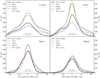 |
Fig. 4 Cuts of the brightness temperature distribution along the east-west axis for real and synthetic observations at four wavelengths. The black solid line in each panel represents the ALMA and VLA observations shown in Fig. 1. The colored lines indicate models with different maximum dust grain sizes, taking values of amax = 10, 100, and 1000 µm. We include models accounting for the sublimation of 80% of the carbonaceous material in the form of refractory organics. The sublimation zone extends over a 10 au radius where the gas temperature exceeds 300 K. The black line under every wavelength label indicates the angular resolution. |
4.2 Effect of carbon sublimation within the soot line
Because the observed brightness temperatures and model dust temperatures are high (≳ 400 K), it might be that some of the dust material gets evaporated within the disk of IRAS 16293 B. The silicate sublimation temperature is around 1200 K, and for graphite, it is 2100 K. Both are well above the central disk temperatures. However, carbon can also exist in nongraphitic forms, for example, amorphous carbon or polyciclyc aromatic hydrocarbons (PAHs) within ice layers. To study the scenario of dust containing refractory carbon that can sublimate at the observed disk temperatures, we also produced synthetic observations with a dust model that includes amorphous carbon. For this we used the optical constants from amorphous carbon (CHON) from Henning & Stognienko (1996) and set a sublimation temperature of 300 K. This temperature is based on the analysis presented by Li et al. (2021), who estimate a temperature range between 200 and 650 K from meteoritic constraints. This range was further narrowed to 300 K by van’t Hoff et al. (2020) after analyzing the relation between sublimation, gas temperature, and pressure at hot-core conditions. The thermodynamic relations they used were derived from PAHs characterized in the lab (Goldfarb & Suuberg 2008; Siddiqi et al. 2009). In our disk model, the soot line at 300 K covers the inner 10 au in radius and ~ 8 au in scale height (see Fig. 2). The extension of this region is also shown with a black scale bar at the bottom of Fig. 4. Details on the dust composition and radiative transfer setup for the inclusion of amorphous carbon are given in Sect. 3.4.
The resulting brightness temperature proiles for the case with carbon sublimation are also shown in Fig. 4 in the form of dashed lines. In the sublimation case, the grain size remains homogeneous, but the composition does not. Outside of the soot line, grains are composed of silicate, graphite, and refractory organics (the opacity is given by the purple line of Fig. 3). Inside the soot line, amorphous carbon is removed, and the composition is the iducial silicate and graphite mixture (turquoise line in Fig. 3), however, with a dust mass reduced by the factor of material sublimated. In Fig. 4, the dashed lines show the case of 80% organics, meaning a dust composition whose carbon budget was split between 20% of graphite and 80% of amorphous carbon while keeping the total carbon budget constant at 37.5% (i.e., with mass fractions of 0.675, 0.300, and 0.075 for silicate, graphite, and amorphous carbon, respectively). We tried different percentages for organics, but we show here only the one with the most signiicant differences from our iducial composition.
The fluxes produced by sublimated grains are not significantly different to those without sublimation, regardless of the size and wavelength or particular amount of organics. As discussed in Sect. 3.4, the sublimation has the effect of lowering the optical depth because of mass reduction and a change in composition. This results in observed emission being produced by a slightly inner and hotter parcel of the disk, which leads to slightly higher fluxes toward the center than the fiducial model without evaporation of the organics. The difference in flux in the central region between models with and without evaporation is larger for the wavelengths with higher-resolution observations.
Our results indicate that detecting dust sublimation with continuum observations at a particular wavelength, even with very high resolution, is challenging. Future observations that are able to obtain molecular line emission from this region will be able to probe whether an active carbon-rich chemistry exists or not in this source (van’t Hoff et al. 2020), providing independent and robust constraints on the scenario of a soot line of about 10 au within this Class 0 disk.
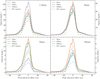 |
Fig. 5 Similar to Fig. 4 but for the optical depth of every radiative transfer model at the ideal resolution. In other words, this is the resolution of the radiative transfer output before any beam convolution. |
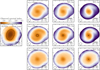 |
Fig. 6 Spectral indexes for the real observation (left) and models (right). Models are shown for amax of 10 μm (top), 100 μm (center), and 1000 μm (bottom). From left to right, the columns represent the cases without sublimation and with 50% and 80% of carbon sublimation, respectively. The black contour indicates α = 2. |
4.3 Variation of the spectral index
Another observable aspect that can be compared between observations and models is the spectral index α produced between our high resolution 1.3 and 3 mm observations. We computed the spectral index between 1.3 and 3 mm for all amax models and for several percentages of organics, 10%, 30%, 50%, and 80%. We present in Fig. 6 our results for models with our fiducial composition, where carbon does not sublimate, and representative sublimation models with 50% and 80% of organics with sublimation temperatures from 300 K.
Since the disk model is optically thick at 1.3 mm and 3 mm (see Fig. 5), the values of the spectral index will depend on the vertical distribution of the temperature and opacity in the disk. The models in Fig. 6 all have the same temperature gradient, but the opacity changes with amax and composition, leading to the observable differences. The models with higher opacities toward the center show a more extended region with α < 2.5 values.
An important feature that has been observed in the IRAS 16293 B spectral index is that central values go as low as 1.7 (first presented in Zamponi et al. 2021). This means a lower value than the threshold of α = 2 (indicated by the black contour in Fig. 6) for optically thick emission. The presence and extent of this feature in our models depends on having sufficient variations of temperature along the line of sight between the layers traced by the different wavelengths (with T1.3mm < T3mm). The larger the region in which these differences are present, the more prominent and widespread the feature is. In the case of 100 μm, the feature is more prominent because of the higher optical depths, while in the case of 1000 μm-sized grains with carbon sublimation, the feature is likely present because the reduced optical depth in the inner hot region allows flux to come from a region with a larger gradient in temperature than the same models with less sublimation. Although none of our models reproduce the extent of this region, models with grain growth are able to reproduce small regions showing this feature (see panels with 100 μm or 1000 μm considering carbon sublimation in Fig. 6).
4.4 Polarization by self-scattering
Polarization toward embedded disks has been interpreted as being caused by self-scattering (Cox et al. 2018; Sadavoy et al. 2018) similar to that observed toward more evolved protoplanetary disks (Kataoka et al. 2016a; Stephens et al. 2017; Lin et al. 2021). This interpretation is based on the morphology of the polarization observations. In this work, we tested whether our disk model with a physical density and temperature structure representative of a Class 0 disk can produce the few percent (2–4%) polarization fractions observed for IRAS 16293 B as well as other Class 0 or Class I disk observations at millimeter wavelengths (Lee et al. 2021). We did so by generating radiative transfer models of polarization by scattering at 1.3 and 7mm. These models were then compared with the available high- resolution polarization data shown in Fig. 1. Creating models of polarization by scattering requires the calculation of full Mie scattering (i.e., Monte Carlo scattering in all four Stokes components) and is highly computationally expensive. Hence, we produced models for all three maximum grain sizes using only our fiducial and homogeneous dust composition of silicates and graphites. Given that the albedo between the different compositions used in this work are very similar, the results at each amax do not deviate significantly when considering the other compositions. Between the three models, the highest polarized intensity is produced by an amax of 100 μm since the albedo of 10 μm grains is negligible and the extinction opacity of 1000 μm-sized grains is larger than that of 100 μm-sized grains (see Table 1) and produces lower scattered flux. Unlike for amax = 10 and 100 μm, the polarization fraction of millimetric grains is very similar at both 1.3 mm and 7 mm in polarization pattern and intensity (maximum Pfrac ~ 0.2%). This is because their albedo is almost constant at all millimetric wavelengths (see Fig. 3). The results of our self-scattering models are presented in Fig. 7 and shown at the disk model’s native resolution. We present the resulting Stokes I, Q, and U fluxes, along with the polarization fraction (and with polarization E-vectors overlaid) at both wavelengths. The resulting Stokes Q and U fluxes at 1.3 mm are extremely low. The polarization fraction in the model reaches around a tenth of a percent (Pfrac ≲ 0.1%) within the central 20 au where it shows an azimuthal polarization pattern for the Evectors. This azimuthal distribution is expected from a centrally concentrated density distribution (Kataoka et al. 2015). In the spiral arms, the vectors become radial or rather perpendicular to these structures. These patterns are similar to those presented by Kataoka et al. (2015) for a ringed and lopsided disk. The fraction of polarization falls significantly at 7 mm, as expected, since it is far from the λ ~ 2πamax regime and barely reaches 0.005% within the disk. We also tested the results for the case of an edge-on hot disk (Fig. B.1). In this case, the polarization fraction remains the highest at 1.3 mm but is consistently low (~ 1%).
Previous ALMA Band 6 polarization observations of IRAS 16293 B from Sadavoy et al. (2018) show an azimuthal Evector pattern with polarization fractions as high as ~ 2% −4 %. Such observations were associated with dust self-scattering. To directly compare these models with IRAS 16293 B observations, we performed polarized synthetic observations at all three Stokes components, mimicking the corresponding observing setups presented in Sect. 2 and the procedure described in Sect. 3.6. The resulting synthetic maps (in units of Jy/beam) are presented in Fig. 8 for both wavelengths and all three Stokes components. In this case, we have omitted the polarization fraction results from the layout because the polarized intensity is completely dominated by thermal noise. The resulting Stokes I fluxes are comparable to the original observations, confirming the analysis presented in Sect. 4.1 but now complemented with the inclusion of the polarized 1.3 mm data. However, the Stokes Q and U model fluxes are not detectable within the sensitivity levels achieved by these observing setups. We concluded from this analysis that the linear polarization produced by self-scattering from spherical grains in our model is not high enough to be consistent with the observations of IRAS16293B carried out at 1.3 and 7 mm by Sadavoy et al. (2018) and Liu et al. (2018), respectively.
Our resulting polarization fractions are in line with the predictions for IRAS 16293 B discussed by Yang et al. (2016) based on analytical models of polarized scattering in optically thick media. The millimeter optical depth in IRAS 16293 B is extremely high (τ ≳ 100), which reduces the degree of anisotropy in the radiation field and hence the percentage of polarized scattered light (Kataoka et al. 2015).
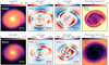 |
Fig. 7 Radiative transfer models of self-scattering at 1.3 (top) and 7 mm (bottom) for amax = 100 μm. From left to right, the panels illustrate the Stokes I, Q, and U fluxes and the polarization fraction (with constant-size polarization vectors overlaid). |
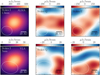 |
Fig. 8 ALMA and VLA synthetic observations based on models of self-scattering from Fig. 7 (i.e., for amax = 100 μm). The polarization fraction panel is omitted since both Q and U components are dominated by thermal noise. The rms of the polarization components are rmsQ ~ rmsU ~ 25 μJy beam−1 and ~12 μJy beam−1 for the 1.3 mm and 7 mm maps, respectively. |
5 Discussion
5.1 Grain growth in Class 0 disks
Grain growth in Class 0 protostars and their associated disks has been a subject of significant interest in recent years. Several recent studies, including Bate (2022), Kawasaki et al. (2022), Koga et al. (2022), Lebreuilly et al. (2023), and Marchand et al. (2023), have provided compelling evidence suggesting the possibility of grain growth up to at least a few hundred microns in these environments. Bate (2022) conducted simulations of prestellar core collapse and followed them until the formation of a rapidly rotating and marginally gravitationally unstable first core. This represents a stage previous to the formation of a well- defined protostellar disk, such as the one in IRAS 16293 B, but shows similar physical properties. Bate (2022) demonstrated that the combination of enhanced collisional rates and efficient grain growth mechanisms can lead to the formation of substantial dust aggregates in Class 0 disks, growing up to 100 μm in this first core stage. These results are in line with our possibility to have particle sizes of 100 μm, or even up to 1000 μm, in a Class 0 disk. Similarly, Kawasaki et al. (2022) evolved one-zone nonideal magnetohydrodynamic models of the collapse of dense cores up to densities comparable to those found in our disk model (ng ≳ 1012 cm−3). Their calculations focused on the evolution of the grain sizes along the collapse, including the effects of coagulation and fragmentation of silicate dust. Their models show that grains can coagulate up to a few 100 microns at the densities of our disk model and therefore at the densities expected in IRAS 16293 B and even up to millimetric sizes within the very inner dense regions of the disk. These results seem to also be in line with our grain-size estimations for the disk in IRAS 16293 B. The similar recent work conducted by Koga et al. (2022) simulated the formation of a protostellar disk with a mass, radius, and age similar to our disk model (i.e., such aspects representative of a Class 0 disk). These simulations did not include dust coagulation but rather fixed grain sizes over the whole evolution. Their results indicate that only the big grains (100–1000 μm) are tightly coupled to the gas within the disk, while small grains (≲10 μm) are partly depleted or swept out from the disk. More recently, Lebreuilly et al. (2023) presented a hydrodynamical simulation of protostellar collapse and followed the evolution of the grain size distribution until the formation of a first core with densities similar to those found by Bate (2022) and in our disk. Their results also suggest that grains can coagulate up to a few tens of microns in the protostellar envelope and up to a few 100 μm within the first core. The results from Marchand et al. (2023) similarly suggest that grain growth is extremely rapid once a disk is formed. Their simulations show how grain sizes can reach more than 100 μm in the inner disk within 1000 years after disk formation. Older predictions for grain sizes in proto- stellar cores, such as those from Ormel et al. (2009), Hirashita & Yan (2009), and Hirashita & Li (2013), suggested that even isothermally collapsing dense cores can achieve coagulation up to 100 μm but only if the cloud’s dynamical support slows down the collapse beyond its freefall time and lets the grains grow. In the case of a collapse faster than the freefall time (≲105 yr), grains should coagulate up to at most a few 10 μm.
Observational constraints from dust emissivity indices also suggest that grains in protostellar (Class 0) envelopes are bigger than in the interstellar medium (ISM), and their maximum sizes could be from few 10 to 1000 μm (Kwon et al. 2009; Agurto-Gangas et al. 2019; Miotello et al. 2014; Bracco et al. 2017; Valdivia et al. 2019; Le Gouellec et al. 2019; Galametz et al. 2019; Hull et al. 2020; Maureira et al. 2022). Itis also worth mentioning that a dust population with maximum grain sizes comparable to ISM values (≲1 μm; Mathis et al. 1977) was not consistent with IRAS 16293 B based on the model-observation comparison presented in Zamponi et al. (2021).
The size distribution is yet another source of uncertainty for comparing models to observations. Although all the theoretical works mentioned above predict significant grain growth in the envelope around Class 0 protostars, and in particular in the high-density material in the disks (e.g., Marchand et al. 2023), the resultant distribution of the grain sizes might be different among different studies (e.g., Bate 2022 and Lebreuilly et al. 2023). While in Lebreuilly et al. (2023), the resultant distribution resembled a power-law, as does the one used in this work, the resultant distribution in Bate (2022) resembled more of a log-normal. This difference can be attributed to how the collision velocities for the grains are calculated (see discussion in Lebreuilly et al. 2023 and Marchand et al. 2023). We found that if we were to consider a log-normal distribution for the grain sizes, the opacities at millimeter wavelengths would slightly increase but still remain within the same order of magnitude as the ones in Fig. 3. Such limited variations cannot help in constraining the dust grain size distribution with our current model, and thus, our conclusions regarding the maximum grain size remain the same regardless of the adopted size distribution.
 |
Fig. 9 Models with grain growth within the sublimation zone. In these models, the maximum grain size is 100 μm outside of the sublimation zone (i.e., in regions where T > 300 K for the upper panels and T > 500 K for the lower panels) and 1000 μm within it, as well as a mixture of silicates, graphites, and amorphous carbon (80% of the carbon). |
5.2 Grain growth within the soot line
The recent VLA observation of FU Ori presented by Liu et al. (2021) showed that within the inner 10 au, where T ≳ 400 K, dust grains have grown to millimeter sizes. Since this region is hot enough for the evaporation of the water ice mantles, this implies that grain growth was efficient in these “dry” conditions. This scenario of grain growth in the inner and hotter regions of protoplanetary disks is also supported by laboratory experiments (Kimura et al. 2020). These experiments show that the stickiness of silicate and carbonaceous grains is enhanced after the removal of quasi-liquid layers of water. This process facilitates dust coagulation and supports the formation of planetesimals in dry environments (Pillich et al. 2021).
The possibility to have millimetric grains can potentially be explained by the high fragmentation velocity vfrag found for water-ice-free grains ≳ 10 m s−1 (Kimura et al. 2015; Gundlach et al. 2018; Steinpilz et al. 2019; Pillich et al. 2021), which is larger than previously considered for rocky, poorly-sticky grains of 1 m s−1 (Blum & Wurm 2000). These results on the fragmentation velocity have also been independently found by Liu et al. (2021) and more recently by Yamamuro et al. (2023).
Motivated by these recent experimental laboratory results, we reproduced synthetic brightness profiles at 1.3 and 3 mm (similar to Fig. 4), accounting for sublimation and grain growth when the temperature is over 300 K. Outside of the sublimation zone, the maximum grain size is 100 μm and the composition is a mixture of silicates, graphites, and refractory organics (80% of the carbon budget). Inside the sublimation zone, we increased the grain size to 1000 pm. The results of this test are shown in Fig. 9 for two different sublimation temperatures, 300 and 500 K, at 1.3 and 3 mm. We present the synthetic ALMA Stokes I maps at the resolution of the observations for comparison with IRAS 16293 B. The brightness profiles resulting from the synthetic images show that the overestimation in the case of amax = 100 μm is mitigated by the reduction of flux in the center when amax = 1000 μm within the soot line. In Fig. 9 we also present the results for two different soot lines in order to explore the effects of considering the range of sublimation temperatures presented by Lin et al. (2021). The fluxes from models with a 500 K soot line are higher than those with 300 K. This happens because with a soot line of 500 K, the region traced by millimetric grains is more compact than the case with 300 K. This means that the region with higher opacity is smaller in the 500 K case. Another observable feature in Fig. 9 is the appearance of a gap in the model with a soot line at 300 K observed at 3 mm. This is caused by the reduction of the opacity, and it is not seen in the model with 500 K because the region with reduced opacity is more compact and less resolved by the observations. This shows that observations of such gaps for hot disks could be the result of changes in the opacity.
Considering grain growth within the soot line results in a better match with the observations than the cases with homogeneous grain sizes. The comparison suggests that grain growth up to millimeter sizes could be enhanced within the soot line in this young Class 0 disk when the disk density temperatures and densities in the model are close to the ones present in IRAS 16293B. Similar results have been found by Xu et al. (2023) toward another typical protostellar disk, TMC1A. Their modeling of multiwavelength observations shows a strong radial dependence of the maximum grain size, regardless of the fragmentation threshold.
5.3 If not self-scattering, what is the polarization mechanism in IRAS 16293-2422 B?
As we showed Sect. 4.4, the emission from IRAS 16293B is too optically thick to produce detectable levels of polarization by self-scattering when considering spherical grains. This raises the question as to what other mechanisms or grain properties can be considered to explain the observed polarization patterns and fractions.
Polarization observations are commonly associated with the optically thin emission of magnetically aligned grains (Lazarian & Hoang 2007a; Andersson et al. 2015). However, the emission detected from young embedded disks is likely optically thick (Galván-Madrid et al. 2018; Lin et al. 2020, 2023; Zamponi et al. 2021; Ohashi et al. 2023). In the context of optically thick emission, the observed polarization might also come from magnetically aligned grains but be produced in the form of extinction (Ko et al. 2020; Liu 2021). In this case, the differential attenuation of the two orthogonal components of the light E-vectors results in an excess of polarization along a given axis (Wood 1997). This is known as dichroic extinction, and it occurs when the grains are elongated and the background light is optically thick and almost unpolarized. In the context of optically thick embedded disks, this can be produced by foreground (e.g., envelope) elongated grains aligned with their minor axis parallel to the magnetic field lines, which preferentially absorb light along the grain’s major axis and produce a net polarization parallel to the magnetic field lines, as opposed to the optically thin polarized emission. Such a polarization mechanism has actually been proposed and detected in a few other Class 0 sources and contradicts the current understanding of magnetic field structures within the optically thick inner regions of the disks (Liu 2021). Similarly, the multiwavelength polarization observations of NGC 1333 IRAS4A presented by Ko et al. (2020) show a transition between E-vectors parallel to the magnetic field, traced at 0.87–1.3 mm, to E-vectors perpendicular to the magnetic field, traced at 6.9–14.1 mm. These results show evidence for a transition between extinction and emission of aligned grains, which is determined by an optically thick-to-thin transition. Similarly, polarization by dichroic extinction has been detected within the inner 100 au of the Class 0 protostar OMC-3/MMS 6 (also known as HOPS-87) in Orion (Liu 2021) after comparing ALMA and VLA observations. Moreover, in the protostar HH212, the polarization observed at a resolution of 14 au shows a possible combined contribution of both dichroic extinction and self-scattering (Lee et al. 2021). Similar results have been found by Kuffmeier et al. (2020) from their numerical simulations of protostellar systems with physical properties similar to IRAS 16293-2422 B. These studies support that dichroic extinction by aligned grains can be an important mechanism to explain the polarization pattern at or close to disk scales in several Class 0 protostars. As this mechanism requires that the region near disk scales be optically thick, it would be preferentially present in younger and more massive disks, such as those in the Class 0 stage.
In the case of IRAS 16293B, the 1.3 mm polarization observations from Sadavoy et al. (2018) show azimuthal E-vectors between 30 and 50au and uniform vectors within 30au (see Fig. 1). In Zamponi et al. (2021) and this work, we show that the emission is optically thick and can reach optical depths well above 100 at 1.3 mm within the central 10 au. If the polarized emission is produced by dichroic extinction of magnetically aligned grains, this pattern would indicate a toroidal magnetic field. Alternatively, the polarization pattern could still be related to the direct emission of magnetically aligned grains close to the disk. The magnetic field morphology (traced by B-vectors) could be associated with a poloidal field in that scenario. Future modeling and higher-resolution observations can help in constraining the contribution of dichroic extinction as well as magnetic field configurations that best explain the observations in Fig. 1.
Another possible scenario producing azimuthal E-vectors similar to those in Fig. 1 is the polarization reversal effect, which happens when millimetric elongated grains are present in the disk and observed in the Mie regime (i.e., millimetric wavelengths). This scenario has been used by Guillet et al. (2020) to explain the azimuthal polarization pattern of [BHB 2007] 11 (the pretzel) in the Pipe nebula, where polarization E-vectors, and so B-vectors, could be aligned with the accretion streamers shown by Alves et al. (2019).
Another scenario is that the polarization can be produced by dust alignment but not necessarily with the magnetic field only. Both the emission and extinction of light from elongated particles rely on the assumption that dust grains are aligned with a given underlying field. This could be either the magnetic, radiation, or velocity field (Gold 1952; Wood 1997; Lazarian 2007). The most commonly accepted mechanisms responsible for the alignment of grains (see Andersson et al. 2015; Reissl et al. 2016 or Hoang et al. 2022 for a review) can either be associated with radiative torques (RAT; Lazarian & Hoang 2007a) or supersonic motions, namely, mechanical torque alignment (also known as MET; Gold 1952; Lazarian & Hoang 2007b; Kataoka et al. 2019; Hoang et al. 2022; Reissl et al. 2023). In the case of RAT, this can lead to alignment with the radiation field (k-RAT; Tazaki et al. 2017) instead of the magnetic field (B-RAT). In the case of mechanical alignment, this could result in alignment with the magnetic field (B-MET) or the velocity field (v-MET; Hoang et al. 2022). In the scenarios of alignment with the radiation (k-RAT) or the dust-gas drift velocity field (v-MET or MAT; Hoang et al. 2018), the resulting polarization pattern would be azimuthal as long as the radiation field is assumed to be centrally concentrated and the disk to be Keplerian (e.g., around a protostar). However, the recent work presented by Le Gouellec et al. (2023) shows that k-RAT is not the main mechanism responsible for the observed polarization in Class 0 protostars since it requires high protostellar luminosities radiating on large and rapidly rotating grains, and such grains are commonly settled toward the midplanes of Class 0 disks, shielded from protostellar radiation. The case of mechanical alignment depends strongly on the Stokes number, that is, the degree of spatial coupling between the gas and the dust. Whether radiation or mechanical alignment are efficient in Class 0 disks requires further investigation.
Finally, given our suggestion of large (>100 μm) grains being present in this Class 0 disk, we found it interesting to consider the scenario of grain rotational disruption induced by radiative torques (RATD), which was introduced by Hoang et al. (2019) and recently discussed by Le Gouellec et al. (2023) and Reissl et al. (2023). According to RATD, large and rapidly rotating aligned grains might become rotationally disrupted when they exceed a certain critical angular momentum and would produce a depletion of grown dust. Le Gouellec et al. (2023) showed that RATD might be effective within the outflow cavity regions of Class 0 protostars for protostellar luminosities above 20 L⊙ and that the densest regions of the disk are well protected against such intense radiative torques. These are the regions where we suggest dust grows to above 100 microns in IRAS 16293B.
6 Conclusions
In this work, we explored the effects of different maximum grain sizes and carbon sublimation in the millimeter continuum emission from a hot and optically thick Class 0 disk generated through numerical simulations of prestellar core collapse. The disk model successfully reproduces the fluxes of the nearly face- on Class 0 disk IRAS 16293 B (Zamponi et al. 2021). Hence, we produced synthetic observations of the different cases to compare with multiwavelength (1.3, 3, 9, and 18 mm) and high- resolution (6 to 44 au) observations of IRAS 16293 B, including polarization observations. To automate the generation of synthetic observations, we developed a new publicly available tool called Synthesizer, which enables the generation of synthetic models from numerical simulations directly from the command line. We summarize the conclusions of this work as follows:
For a dust mixture of silicates and graphites, we extended the results of Zamponi et al. (2021), which used maximum grain sizes amax of 1 μm and 10 μm and generated opacity tables for maximum grain sizes of up to 100 μm and 1000 μm. From the synthetic brightness profiles, peak fluxes increase with wavelength and decrease with amax, a feature of hot and optically thick disks. Optical depths range between 130 and 2 from 1.3 to 18 mm, respectively. The high optical depths and positive temperature gradient toward the center also result in extended regions in the disk, with α < 2.5 for all amax and even below 2 for amax = 100 μm and 1000 μm. Predictions from significant grain growth populations including amax = 1000 μm are comparable to the observations from IRAS 16293 B at all observed wavelengths. Hence, significant grain growth could be present in this young Class 0 disk;
Motivated by the high brightness temperatures (≳400 K) observed toward IRAS 16293 B, we explored the scenario of sublimation of solid amorphous refractory carbon at temperatures above 300 K, the so-called soot line. The sublimation results in a local decrease of the optical depth, due to both the reduction of graphite within the grain carbon budget and the evaporated mass reduction. This decrease produces higher fluxes because the emission then traces deeper and hotter layers of the disk. The difference in the fluxes with and without sublimation are small (<10%);
We also tested the hypothetical case of grain growth within the soot line, motivated by recent laboratory experiments suggesting that dry grains without ice mantles would enhance stickiness and coagulation. We modeled this scenario with an amax of 100 μm at all disk scales outside of the soot line and with millimetric grains within it. Our results indicate that a combination of both grain sizes can help provide a better match to the ALMA observations of IRAS 16293 B;
We generated polarization models by self-scattering for three different maximum grain sizes, 10, 100, and 1000 μm. The millimetric polarized intensity is the highest for the case with amax = 100 μm at 1.3 mm due to a high albedo and a not extremely high optical depth, as it happens for millimetric grains. However, the predicted polarization fraction produced by self-scattering is very low (≲0.5%) for both the edge-on and face-on disks. These low levels of polarization by self-scattering are too low to be consistent with those observed for IRAS 16293 B at both 1.3 mm and 7mm (2–4%).
Since self-scattering is unlikely to be at the origin of the high- polarization fractions observed toward the Class 0 disk IRAS 16293 B, further modeling in the future is needed to constraint the mechanism responsible for the observed polarization. Similar studies toward other embedded disks would be useful to see if this is a general result for other Class 0 disks. Higher- resolution molecular observations would also help investigate whether there is enriched carbon chemistry in the inner regions of the disk.
Acknowledgements
We thank the anonymous referee for the constructive feedback that led to significant improvement of this manuscript. We also thank Cornelis Dullemond, Robert Brunngräber, Tommaso Grassi, John D. Ilee, Michael Küffmeier and Valentin Le Gouellec for help building the setup and implementation of this project. J.Z., M.J.M., B.Z., D.S. and P.C. acknowledge the financial support of the Max Planck Society. H.B.L. is supported by the National Science and Technology Council (NSTC) of Taiwan (Grant Nos. 111-2112-M-110-022-MY3). D.S. is supported by an NSF Astronomy and Astrophysics Postdoctoral Fellowship under award AST-2102405. This paper makes use of ALMA data from the following projects: 2015.1.01112.S (PI: S. Sadavoy), 2017.1.01247.S (PI: G. Dipierro) and 2016.1.00457.S (PI: Y. Oya). ALMA is a partnership of ESO (representing its member states), NSF (USA) and NINS (Japan), together with NRC (Canada), MOST and ASIAA (Taiwan), and KASI (Republic of Korea), in cooperation with the Republic of Chile. The Joint ALMA Observatory is operated by ESO, AUI NRAO and NAOJ. The National Radio Astronomy Observatory is a facility of the National Science Foundation operated under cooperative agreement by Associated Universities, Inc. This research made use of Astropy: a community-developed core Python package and an ecosystem of tools and resources for astronomy (Astropy Collaboration 2013, 2018; Astropy Collaboration et al. 2022), APLpy: an open-source plotting package for Python (Robitaille & Bressert 2012), NumPy: an open source project that enables numerical computing with Python (Harris et al. 2020), Matplotlib: a 2D graphics environment (Hunter 2007) and Mayavi: an open-source library for 3D rendering in Python (Ramachandran & Varoquaux 2011).
Appendix A The DustMixer: A command-line tool to generate dust opacities
DUSTMIXER is a module contained within Synthesizer designed to handle the mixing of different dust compositions and to calculate opacities. Its implementation is partly based on another publicly available and useful tool to compute dust opacities called OpTool (Dominik et al. 2021) and DSHARP_OPAC (Birnstiel et al. 2018). A reimplementation of a similar module was done to allow the module to be cleanly embedded within SYNTHESIZER and to access its command line interface.
The DUSTMIXER reads in tabulated optical constants n and k (also called refractive indices) for a given material. It interpolates the entered values over a user-defined wavelength grid and extrapolates if necessary. The extrapolations are done as a constant, and as a power-law for both the lower and upper wavelength bounds, respectively. Then, it uses the BHMIE algorithm (Bohren & Huffman 1983) to convert these constants into extinction and scattering dust efficiencies, Qext and Qsca, as well as scattering matrix components for all wavelengths and a single grain size. This algorithm calculates scattering efficiencies by assuming that re-emitted (scattered) photons can be modeled as the expansion of vector spherical harmonics. This calculation involves solving infinite Riccati-Bessel functions and is highly computationally expensive. The larger the grain size compared to the wavelength, the greater the number of terms that need to be added in the series and therefore the longer the calculation. The SYNTHESIZER employs a multiprocessing scheme to calculate these efficiencies within minutes for a proper resolution (200 wavelengths and 200 grain sizes; see Fig. 3). Finally, to obtain dust opacities, all single grain size efficiencies are integrated over a power law size distribution within a minimum amin and maximum amax grain size for a given power law slope q.
To combine different dust compositions, several mixing methods exist in the literature. Some of them directly mix the refractive indices using mixing rules, such as the Brugemann or Maxwell-Garnet rules (see e.g., Birnstiel et al. 2018), and create a new homogeneous sphere of mixed material to calculate the opacities. Other methods use effective medium theories and consider layered dust grains composed of a core and a mantle (e.g., Ossenkopf 1991; Ossenkopf & Henning 1994) to calculate the opacities of grains with different core-mantle volume ratios. The DUSTMIXER provides support for both mixing techniques. However, in this work, we calculated opacities per material and combined them as a sum weighted by their mass fractions (see Sect. 3.4), meaning different materials coexist within the grid cells and lead to a net opacity rather than merging into an alloy. More details about this tool and its additional functionalities can be found in its public repository.
Appendix B Polarization models by self-scattering for an edge-on hot disk
In this appendix, we present polarized radiative transfer models produced by self-scattering that are similar to those presented in Sect. 3.5 and shown in Fig. 7, but this time the models use an edge-on projection for the same disk model. Our aim is to provide more global predictions for self-scattering polarization in early embedded Class 0 disks rather than only the case of the nearly face-on disk on IRAS 16293 B. The results of this model are shown in Fig. B.1 for our fiducial dust population of silicates and graphites with amax = 100 μm, analogous to the case in Fig. 7. The polarization fraction of the edge-on models is slightly larger than for the face-on projection (≲ 1%) but still low enough to match the ALMA and JVLA observations from Fig. 1.
 |
Fig. B.1 Radiative transfer models of self-scattering at 1.3 (top) and 7 mm (bottom) for amax = 100 μm, shown in the upper and lower row, respectively. This figure is similar to Fig. 7 but shows an edge-on projection of the same hot and massive disk model. |
References
- Agurto-Gangas, C., Pineda, J. E., Szűcs, L., et al. 2019, A&A, 623, A147 [NASA ADS] [CrossRef] [EDP Sciences] [Google Scholar]
- Alves, F. O., Caselli, P., Girart, J. M., et al. 2019, Science, 366, 90 [NASA ADS] [CrossRef] [Google Scholar]
- Andersson, B. G., Lazarian, A., & Vaillancourt, J. E. 2015, ARA&A, 53, 501 [Google Scholar]
- Andre, P., Ward-Thompson, D., & Barsony, M. 1993, ApJ, 406, 122 [NASA ADS] [CrossRef] [Google Scholar]
- Andrews, S. M. 2020, ARA&A, 58, 483 [Google Scholar]
- Astropy Collaboration (Robitaille, T. P., et al.) 2013, A&A, 558, A33 [NASA ADS] [CrossRef] [EDP Sciences] [Google Scholar]
- Astropy Collaboration (Price-Whelan, A. M., et al.) 2018, AJ, 156, 123 [Google Scholar]
- Astropy Collaboration (Price-Whelan, A. M., et al.) 2022, ApJ, 935, 167 [NASA ADS] [CrossRef] [Google Scholar]
- Avenhaus, H., Quanz, S. P., Garufi, A., et al. 2018, ApJ, 863, 44 [NASA ADS] [CrossRef] [Google Scholar]
- Ballering, N. P., & Eisner, J. A. 2019, AJ, 157, 144 [Google Scholar]
- Bate, M. R. 2022, MNRAS, 514, 2145 [CrossRef] [Google Scholar]
- Bate, M. R., Bonnell, I. A., & Price, N. M. 1995, MNRAS, 277, 362 [Google Scholar]
- Birnstiel, T., Dullemond, C. P., Zhu, Z., et al. 2018, ApJ, 869, L45 [CrossRef] [Google Scholar]
- Bjorkman, J. E., & Wood, K. 2001, ApJ, 554, 615 [NASA ADS] [CrossRef] [Google Scholar]
- Blum, J., & Wurm, G. 2000, Icarus, 143, 138 [NASA ADS] [CrossRef] [Google Scholar]
- Bohren, C. F., & Huffman, D. R. 1983, Absorption and scattering of light by small particles (New York: Wiley) [Google Scholar]
- Bracco, A., Palmeirim, P., André, P., et al. 2017, A&A, 604, A52 [NASA ADS] [CrossRef] [EDP Sciences] [Google Scholar]
- Cox, E. G., Harris, R. J., Looney, L. W., et al. 2018, ApJ, 855, 92 [NASA ADS] [CrossRef] [Google Scholar]
- Dipierro, G., Lodato, G., Testi, L., & de Gregorio Monsalvo, I. 2014, MNRAS, 444, 1919 [Google Scholar]
- Dominik, C., Min, M., & Tazaki, R. 2021, Astrophysics Source Code Library, [record ascl:2104.010] [Google Scholar]
- Draine, B. T. 2003a, ApJ, 598, 1017 [NASA ADS] [CrossRef] [Google Scholar]
- Draine, B. T. 2003b, ApJ, 598, 1026 [NASA ADS] [CrossRef] [Google Scholar]
- Dullemond, C. P., Juhasz, A., Pohl, A., et al. 2012, Astrophysics Source Code Library, [record ascl:1202.015] [Google Scholar]
- Dzib, S. A., Ortiz-León, G. N., Hernández-Gómez, A., et al. 2018, A&A, 614, A20 [NASA ADS] [CrossRef] [EDP Sciences] [Google Scholar]
- Galametz, M., Maury, A. J., Valdivia, V., et al. 2019, A&A, 632, A5 [NASA ADS] [CrossRef] [EDP Sciences] [Google Scholar]
- Galván-Madrid, R., Liu, H. B., Izquierdo, A. F., et al. 2018, ApJ, 868, 39 [CrossRef] [Google Scholar]
- Garufi, A., Benisty, M., Pinilla, P., et al. 2018, A&A, 620, A94 [NASA ADS] [CrossRef] [EDP Sciences] [Google Scholar]
- Garufi, A., Podio, L., Bacciotti, F., et al. 2019, A&A, 628, A68 [NASA ADS] [CrossRef] [EDP Sciences] [Google Scholar]
- Garufi, A., Avenhaus, H., Pérez, S., et al. 2020, A&A, 633, A82 [NASA ADS] [CrossRef] [EDP Sciences] [Google Scholar]
- Gold, T. 1952, MNRAS, 112, 215 [NASA ADS] [Google Scholar]
- Goldfarb, J. L., & Suuberg, E. M. 2008, J. Chem. Eng. Data, 53, 670 [CrossRef] [Google Scholar]
- Guillet, V., Girart, J. M., Maury, A. J., & Alves, F. O. 2020, A&A, 634, L15 [NASA ADS] [CrossRef] [EDP Sciences] [Google Scholar]
- Gundlach, B., Schmidt, K. P., Kreuzig, C., et al. 2018, MNRAS, 479, 1273 [NASA ADS] [CrossRef] [Google Scholar]
- Harris, R. J., Cox, E. G., Looney, L. W., et al. 2018, ApJ, 861, 91 [Google Scholar]
- Harris, C. R., Millman, K. J., van der Walt, S. J., et al. 2020, Nature, 585, 357 [NASA ADS] [CrossRef] [Google Scholar]
- Henning, T., & Stognienko, R. 1996, A&A, 311, 291 [NASA ADS] [Google Scholar]
- Henyey, L. G., & Greenstein, J. L. 1941, ApJ, 93, 70 [Google Scholar]
- Hernández-Gómez, A., Loinard, L., Chandler, C. J., et al. 2019, ApJ, 875, 94 [Google Scholar]
- Hirashita, H., & Yan, H. 2009, MNRAS, 394, 1061 [Google Scholar]
- Hirashita, H., & Li, Z. Y. 2013, MNRAS, 434, L70 [CrossRef] [Google Scholar]
- Hoang, T., Cho, J., & Lazarian, A. 2018, ApJ, 852, 129 [NASA ADS] [CrossRef] [Google Scholar]
- Hoang, T., Tram, L. N., Lee, H., & Ahn, S.-H. 2019, Nat. Astron., 3, 766 [Google Scholar]
- Hoang, T., Tram, L. N., Phan, V. H. M., et al. 2022, AJ, 164, 248 [NASA ADS] [CrossRef] [Google Scholar]
- Hull, C. L. H., Le Gouellec, V. J. M., Girart, J. M., Tobin, J. J., & Bourke, T. L. 2020, ApJ, 892, 152 [NASA ADS] [CrossRef] [Google Scholar]
- Hunter, J. D. 2007, Comput. Sci. Eng., 9, 90 [NASA ADS] [CrossRef] [Google Scholar]
- Jager, C., Mutschke, H., & Henning, T. 1998, A&A, 332, 291 [Google Scholar]
- Jørgensen, J. K., van der Wiel, M. H. D., Coutens, A., et al. 2016, A&A, 595, A117 [Google Scholar]
- Kataoka, A., Muto, T., Momose, M., et al. 2015, ApJ, 809, 78 [Google Scholar]
- Kataoka, A., Muto, T., Momose, M., Tsukagoshi, T., & Dullemond, C. P. 2016a, ApJ, 820, 54 [NASA ADS] [CrossRef] [Google Scholar]
- Kataoka, A., Tsukagoshi, T., Momose, M., et al. 2016b, ApJ, 831, L12 [Google Scholar]
- Kataoka, A., Tsukagoshi, T., Pohl, A., et al. 2017, ApJ, 844, L5 [Google Scholar]
- Kataoka, A., Okuzumi, S., & Tazaki, R. 2019, ApJ, 874, L6 [CrossRef] [Google Scholar]
- Kawasaki, Y., Koga, S., & Machida, M. N. 2022, MNRAS, 515, 2072 [NASA ADS] [CrossRef] [Google Scholar]
- Kimura, H., Wada, K., Senshu, H., & Kobayashi, H. 2015, ApJ, 812, 67 [NASA ADS] [CrossRef] [Google Scholar]
- Kimura, H., Wada, K., Kobayashi, H., et al. 2020, MNRAS, 498, 1801 [Google Scholar]
- Ko, C.-L., Liu, H. B., Lai, S.-P., et al. 2020, ApJ, 889, 172 [NASA ADS] [CrossRef] [Google Scholar]
- Koga, S., Kawasaki, Y., & Machida, M. N. 2022, MNRAS, 515, 6073 [NASA ADS] [CrossRef] [Google Scholar]
- Kress, M. E., Tielens, A. G. G. M., & Frenklach, M. 2010, Adv. Space Res., 46, 44 [NASA ADS] [CrossRef] [Google Scholar]
- Kuffmeier, M., Reissl, S., Wolf, S., Stephens, I., & Calcutt, H. 2020, A&A, 639, A137 [NASA ADS] [CrossRef] [EDP Sciences] [Google Scholar]
- Kwon, W., Looney, L. W., Mundy, L. G., Chiang, H.-F., & Kemball, A. J. 2009, ApJ, 696, 841 [NASA ADS] [CrossRef] [Google Scholar]
- Lazarian, A. 2007, J. Quant. Spec. Radiat. Transf., 106, 225 [NASA ADS] [CrossRef] [Google Scholar]
- Lazarian, A., & Hoang, T. 2007a, MNRAS, 378, 910 [NASA ADS] [CrossRef] [Google Scholar]
- Lazarian, A., & Hoang, T. 2007b, ApJ, 669, L77 [NASA ADS] [CrossRef] [Google Scholar]
- Lebreuilly, U., Vallucci-Goy, V., Guillet, V., Lombart, M., & Marchand, P. 2023, MNRAS, 518, 3326 [Google Scholar]
- Lee, C.-F., Li, Z.-Y., Yang, H., et al. 2021, ApJ, 910, 75 [NASA ADS] [CrossRef] [Google Scholar]
- Le Gouellec, V. J. M., Hull, C. L. H., Maury, A. J., et al. 2019, ApJ, 885, 106 [NASA ADS] [CrossRef] [Google Scholar]
- Le Gouellec, V. J. M., Maury, A. J., Hull, C. L. H., et al. 2023, A&A, 675, A133 [NASA ADS] [CrossRef] [EDP Sciences] [Google Scholar]
- Li, J., Bergin, E. A., Blake, G. A., Ciesla, F. J., & Hirschmann, M. M. 2021, Sci. Adv., 7, eabd3632 [NASA ADS] [CrossRef] [Google Scholar]
- Lin, Z.-Y. D., Li, Z.-Y., Yang, H., et al. 2020, MNRAS, 493, 4868 [Google Scholar]
- Lin, Z.-Y. D., Lee, C.-F., Li, Z.-Y., Tobin, J. J., & Turner, N. J. 2021, MNRAS, 501, 1316 [Google Scholar]
- Lin, Z.-Y. D., Li, Z.-Y., Tobin, J. J., et al. 2023, ApJ, 951, 9 [NASA ADS] [CrossRef] [Google Scholar]
- Liu, H. B. 2021, ApJ, 914, 25 [NASA ADS] [CrossRef] [Google Scholar]
- Liu, H. B., Hasegawa, Y., Ching, T.-C., et al. 2018, A&A, 617, A3 [NASA ADS] [CrossRef] [EDP Sciences] [Google Scholar]
- Liu, H. B., Tsai, A.-L., Chen, W. P., et al. 2021, ApJ, 923, 270 [NASA ADS] [CrossRef] [Google Scholar]
- Marchand, P., Lebreuilly, U., Mac Low, M. M., & Guillet, V. 2023, A&A, 670, A61 [NASA ADS] [CrossRef] [EDP Sciences] [Google Scholar]
- Mathis, J. S., Rumpl, W., & Nordsieck, K. H. 1977, ApJ, 217, 425 [Google Scholar]
- Maureira, M. J., Pineda, J. E., Segura-Cox, D. M., et al. 2020, ApJ, 897, 59 [NASA ADS] [CrossRef] [Google Scholar]
- Maureira, M. J., Gong, M., Pineda, J. E., et al. 2022, ApJ, 941, L23 [NASA ADS] [CrossRef] [Google Scholar]
- Maury, A. J., André, P., Testi, L., et al. 2019, A&A, 621, A76 [NASA ADS] [CrossRef] [EDP Sciences] [Google Scholar]
- McMullin, J. P., Waters, B., Schiebel, D., Young, W., & Golap, K. 2007, ASP Conf. Ser., 376, 127 [Google Scholar]
- Michel, A., Sadavoy, S. I., Sheehan, P. D., et al. 2023, AJ, 166, 184 [NASA ADS] [CrossRef] [Google Scholar]
- Mie, G. 1908, Ann. Phys., 330, 377 [Google Scholar]
- Miotello, A., Testi, L., Lodato, G., et al. 2014, A&A, 567, A32 [NASA ADS] [CrossRef] [EDP Sciences] [Google Scholar]
- Ohashi, S., Kataoka, A., van der Marel, N., et al. 2020, ApJ, 900, 81 [Google Scholar]
- Ohashi, N., Tobin, J. J., Jørgensen, J. K., et al. 2023, ApJ, 951, 8 [NASA ADS] [CrossRef] [Google Scholar]
- Ormel, C. W., Paszun, D., Dominik, C., & Tielens, A. G. G. M. 2009, A&A, 502, 845 [NASA ADS] [CrossRef] [EDP Sciences] [Google Scholar]
- Ossenkopf, V. 1991, A&A, 251, 210 [NASA ADS] [Google Scholar]
- Ossenkopf, V., & Henning, T. 1994, A&A, 291, 943 [NASA ADS] [Google Scholar]
- Pillich, C., Bogdan, T., Landers, J., Wurm, G., & Wende, H. 2021, A&A, 652, A106 [NASA ADS] [CrossRef] [EDP Sciences] [Google Scholar]
- Ramachandran, P., & Varoquaux, G. 2011, Comput. Sci. Eng., 13, 40 [NASA ADS] [CrossRef] [Google Scholar]
- Rao, R., Girart, J. M., Marrone, D. P., Lai, S.-P., & Schnee, S. 2009, ApJ, 707, 921 [NASA ADS] [CrossRef] [Google Scholar]
- Rao, R., Girart, J. M., Lai, S.-P., & Marrone, D. P. 2014, ApJ, 780, L6 [Google Scholar]
- Reissl, S., Wolf, S., & Brauer, R. 2016, A&A, 593, A87 [NASA ADS] [CrossRef] [EDP Sciences] [Google Scholar]
- Reissl, S., Meehan, P., & Klessen, R. S. 2023, A&A, 674, A47 [NASA ADS] [CrossRef] [EDP Sciences] [Google Scholar]
- Robitaille, T., & Bressert, E. 2012, Astrophysics Source Code Library, [record ascl:1200.017] [Google Scholar]
- Rodríguez, L. F., Loinard, L., D’Alessio, P., Wilner, D. J., & Ho, P. T. P. 2005, ApJ, 621, L133 [CrossRef] [Google Scholar]
- Sadavoy, S. I., Myers, P. C., Stephens, I. W., et al. 2018, ApJ, 869, 115 [NASA ADS] [CrossRef] [Google Scholar]
- Sadavoy, S. I., Stephens, I. W., Myers, P. C., et al. 2019, ApJS, 245, 2 [Google Scholar]
- Segura-Cox, D. M., Looney, L. W., Tobin, J. J., et al. 2018, ApJ, 866, 161 [Google Scholar]
- Segura-Cox, D. M., Schmiedeke, A., Pineda, J. E., et al. 2020, Nature, 586, 228 [NASA ADS] [CrossRef] [Google Scholar]
- Sheehan, P. D., & Eisner, J. A. 2018, ApJ, 857, 18 [NASA ADS] [CrossRef] [Google Scholar]
- Siddiqi, M. A., Siddiqui, R. A., & Atakan, B. 2009, J. Chem. Eng. Data, 54, 2795 [CrossRef] [Google Scholar]
- Silsbee, K., Ivlev, A. V., Sipilä, O., Caselli, P., & Zhao, B. 2020, A&A, 641, A39 [NASA ADS] [CrossRef] [EDP Sciences] [Google Scholar]
- Simmons, J. F. L., & Stewart, B. G. 1985, A&A, 142, 100 [NASA ADS] [Google Scholar]
- Steinacker, J., Baes, M., & Gordon, K. D. 2013, ARA&A, 51, 63 [CrossRef] [Google Scholar]
- Steinpilz, T., Teiser, J., & Wurm, G. 2019, ApJ, 874, 60 [NASA ADS] [CrossRef] [Google Scholar]
- Stephens, I. W., Yang, H., Li, Z.-Y., et al. 2017, ApJ, 851, 55 [Google Scholar]
- Tazaki, R., Lazarian, A., & Nomura, H. 2017, ApJ, 839, 56 [NASA ADS] [CrossRef] [Google Scholar]
- Testi, L., Birnstiel, T., Ricci, L., et al. 2014, in Protostars and Planets VI, eds. H. Beuther, R. S. Klessen, C. P. Dullemond, & T. Henning, 339 [Google Scholar]
- Tsukamoto, Y., Maury, A., Commerçon, B., et al. 2022, ArXiv e-prints [arXiv:2209.13765] [Google Scholar]
- Tychoniec, Ł., Manara, C. F., Rosotti, G. P., et al. 2020, A&A, 640, A19 [NASA ADS] [CrossRef] [EDP Sciences] [Google Scholar]
- Vaillancourt, J. E. 2006, PASP, 118, 1340 [Google Scholar]
- Valdivia, V., Maury, A., Brauer, R., et al. 2019, MNRAS, 488, 4897 [NASA ADS] [CrossRef] [Google Scholar]
- van’t Hoff, M. L. R., Bergin, E. A., Jørgensen, J. K., & Blake, G. A. 2020, ApJ, 897, L38 [CrossRef] [Google Scholar]
- Weidenschilling, S. J. 1977, MNRAS, 180, 57 [Google Scholar]
- Wolf, S., & Voshchinnikov, N. V. 2004, Comput. Phys. Commun., 162, 113 [Google Scholar]
- Wood, K. 1997, ApJ, 477, L25 [NASA ADS] [CrossRef] [Google Scholar]
- Xu, W. 2022, ApJ, 934, 156 [NASA ADS] [CrossRef] [Google Scholar]
- Xu, W., & Kunz, M. W. 2021a, MNRAS, 502, 4911 [NASA ADS] [CrossRef] [Google Scholar]
- Xu, W., & Kunz, M. W. 2021b, MNRAS, 508, 2142 [NASA ADS] [CrossRef] [Google Scholar]
- Xu, W., Ohashi, S., Aso, Y., & Liu, H. B. 2023, ApJ, 954, 190 [NASA ADS] [CrossRef] [Google Scholar]
- Yamamuro, R., Tanaka, K. E. I., & Okuzumi, S. 2023, ApJ, 949, 29 [NASA ADS] [CrossRef] [Google Scholar]
- Yang, H., & Li, Z.-Y. 2020, ApJ, 889, 15 [Google Scholar]
- Yang, H., Li, Z.-Y., Looney, L., & Stephens, I. 2016, MNRAS, 456, 2794 [Google Scholar]
- Yang, H., Li, Z.-Y., Looney, L. W., Girart, J. M., & Stephens, I. W. 2017, MNRAS, 472, 373 [Google Scholar]
- Zamponi, J., Maureira, M. J., Zhao, B., et al. 2021, MNRAS, 508, 2583 [NASA ADS] [CrossRef] [Google Scholar]
- Zhao, B., Caselli, P., Li, Z.-Y., & Krasnopolsky, R. 2018, MNRAS, 473, 4868 [Google Scholar]
- Zubko, V., Dwek, E., & Arendt, R. G. 2004, ApJS, 152, 211 [NASA ADS] [CrossRef] [Google Scholar]
We acknowledge that the presence of refractory organics in the icy mantles of dust grains should in principle not affect the content of core carbon (i.e., graphite) and that a proper sublimation model should evaporate the refractory carbon without affecting the graphitic core. However, the nature of the mixing process in our setup (see Sect. 3.2) forces us to reduce the mass fractions of some materials to account for the inclusion of others while keeping the dust mass constant.
All Tables
Dust opacities (g cm−2) used in this work for different maximum grain sizes, for different compositions, and at four wavelengths.
All Figures
|
Fig. 1 IRAS 16293-2422 B observed at ALMA bands 6 and 3 and VLA bands Q, Ka, and Ku (from left to right). The cyan vectors represent polarization E-vectors (masked out below 3σI and 3σQ), and the scale bar indicates a 2% polarization fraction. The continuum data at 1.3 and 3 mm were presented by Zamponi et al. (2021), and the 1.3 mm polarization observations were presented by Sadavoy et al. (2018). The polarized continuum observations at 7 mm were obtained from Liu et al. (2018). The 9 mm and 18 mm continuum observations are presented for the first time by this work. The angular resolution of the observations are as follows: 0.114″ × 0.069″ at 1.3 mm (0.18″ × 0.09″ for polarized data); 0.048″ × 0.046″ at 3 mm; 0.39″ × 0.24″ at 7 mm; 0.12″ × 0.05″ at 9 mm; and 0.23″ × 0.09″ at 18 mm. |
| In the text | |
|
Fig. 2 Face-on gas density (top) and edge-on temperature (bottom) distributions across the midplane of the protostellar disk formed from the numerical simulations of the collapse of a core. We note that this is the disk we compared to the observations of IRAS 16293-2422 B. The white contour in the bottom panel represents the extension of the soot line at 300 K. This model is presented in greater detail in Zamponi et al. (2021). |
| In the text | |
|
Fig. 3 Dust opacities for different maximum grain sizes and compositions. The three panels show, from left to right, dust opacities for a maximum grain size of 10, 100 & 1000 µm, respectively. Each panel contains opacities generated for a mixture of silicates and graphite (0.625–0.375) and a mixture of silicates, graphites and refractory organics (0.627–0.300–0.075; 80% of organics). The gray curve on every panel indicates the albedo of the fiducial composition (silicates and graphites). Four vertical gray lines indicate the observing wavelengths used in this study, corresponding to the observations from Fig. 1. The exact opacity values used in this work are listed in Table 1, for different amax and compositions, at all four wavelengths. |
| In the text | |
|
Fig. 4 Cuts of the brightness temperature distribution along the east-west axis for real and synthetic observations at four wavelengths. The black solid line in each panel represents the ALMA and VLA observations shown in Fig. 1. The colored lines indicate models with different maximum dust grain sizes, taking values of amax = 10, 100, and 1000 µm. We include models accounting for the sublimation of 80% of the carbonaceous material in the form of refractory organics. The sublimation zone extends over a 10 au radius where the gas temperature exceeds 300 K. The black line under every wavelength label indicates the angular resolution. |
| In the text | |
|
Fig. 5 Similar to Fig. 4 but for the optical depth of every radiative transfer model at the ideal resolution. In other words, this is the resolution of the radiative transfer output before any beam convolution. |
| In the text | |
|
Fig. 6 Spectral indexes for the real observation (left) and models (right). Models are shown for amax of 10 μm (top), 100 μm (center), and 1000 μm (bottom). From left to right, the columns represent the cases without sublimation and with 50% and 80% of carbon sublimation, respectively. The black contour indicates α = 2. |
| In the text | |
|
Fig. 7 Radiative transfer models of self-scattering at 1.3 (top) and 7 mm (bottom) for amax = 100 μm. From left to right, the panels illustrate the Stokes I, Q, and U fluxes and the polarization fraction (with constant-size polarization vectors overlaid). |
| In the text | |
|
Fig. 8 ALMA and VLA synthetic observations based on models of self-scattering from Fig. 7 (i.e., for amax = 100 μm). The polarization fraction panel is omitted since both Q and U components are dominated by thermal noise. The rms of the polarization components are rmsQ ~ rmsU ~ 25 μJy beam−1 and ~12 μJy beam−1 for the 1.3 mm and 7 mm maps, respectively. |
| In the text | |
|
Fig. 9 Models with grain growth within the sublimation zone. In these models, the maximum grain size is 100 μm outside of the sublimation zone (i.e., in regions where T > 300 K for the upper panels and T > 500 K for the lower panels) and 1000 μm within it, as well as a mixture of silicates, graphites, and amorphous carbon (80% of the carbon). |
| In the text | |
|
Fig. B.1 Radiative transfer models of self-scattering at 1.3 (top) and 7 mm (bottom) for amax = 100 μm, shown in the upper and lower row, respectively. This figure is similar to Fig. 7 but shows an edge-on projection of the same hot and massive disk model. |
| In the text | |
Current usage metrics show cumulative count of Article Views (full-text article views including HTML views, PDF and ePub downloads, according to the available data) and Abstracts Views on Vision4Press platform.
Data correspond to usage on the plateform after 2015. The current usage metrics is available 48-96 hours after online publication and is updated daily on week days.
Initial download of the metrics may take a while.