| Issue |
A&A
Volume 681, January 2024
|
|
|---|---|---|
| Article Number | A9 | |
| Number of page(s) | 12 | |
| Section | Atomic, molecular, and nuclear data | |
| DOI | https://doi.org/10.1051/0004-6361/202347437 | |
| Published online | 20 December 2023 | |
Water ice: Temperature-dependent refractive indexes and their astrophysical implications
1
Laboratory for Astrophysics, Leiden Observatory, Leiden University,
PO Box 9513,
2300 RA
Leiden,
The Netherlands
e-mail: This email address is being protected from spambots. You need JavaScript enabled to view it.
2
Leiden Observatory, Leiden University,
PO Box 9513,
2300 RA
Leiden,
The Netherlands
3
Max Planck Institute for Astronomy,
Königstuhl 17,
69117
Heidelberg,
Germany
4
Van’t Hoff Institute for Molecular Sciences, University of Amsterdam,
Science Park 904,
1098XH
Amsterdam,
The Netherlands
Received:
11
July
2023
Accepted:
23
August
2023
Abstract
Context. Interstellar and circumstellar ices are largely composed of frozen water. Therefore, it is important to derive fundamental parameters for H2O ice such as absorption and scattering opacities, for which accurate complex refractive indexes are needed.
Aims. The primary goal of the work presented here is to derive ice-grain opacities based on accurate H2O ice complex refractive indexes at low temperatures and to assess the impact this has on the derivation of water ice column densities and porosity in space.
Methods. We used the optool code to derive ice-grain scattering and absorption opacity values based on new and previously reported mid-infrared (mid-IR) complex refractive index measurements of H2O ice, primarily in its amorphous form, but not exclusively. Next, we used those opacities in the RADMC-3D code to run a radiative transfer simulation of a protostellar envelope containing H2O ice, which was then used to calculate water ice column densities.
Results. We found that the real refractive index in the mid-IR of H2O ice at 30 K is ~14% lower than previously reported in the literature. This has a direct impact on the ice column densities derived from the simulations of embedded protostars. Additionally, we found that ice porosity plays a significant role in the opacity of icy grains and that the H2O libration mode can be used as a diagnostic tool to constrain the porosity level. Finally, the refractive indexes presented here allowed us to estimate a grain size detection limit of 18 μm based on the 3 μm band, whereas the 6 μm band allowed us to trace grain sizes larger than 20 μm.
Conclusions. Based on radiative transfer simulations using new mid-IR refractive indexes, we conclude that H2O ice leads to more absorption of infrared light than previously estimated. This implies that the 3 and 6 μm bands remain detectable in icy grains with sizes larger than 10 μm. Finally, we also propose that the H2O ice libration band can be used as a diagnostic tool to constrain the porosity level of the interstellar ice, in addition to the OH dangling bond, which is now routinely used for this purpose.
Key words: solid state: volatile / infrared: ISM / astrochemistry
© The Authors 2023
 Open Access article, published by EDP Sciences, under the terms of the Creative Commons Attribution License (https://creativecommons.org/licenses/by/4.0), which permits unrestricted use, distribution, and reproduction in any medium, provided the original work is properly cited.
This article is published in open access under the Subscribe to Open model. This email address is being protected from spambots. You need JavaScript enabled to view it. to support open access publication.
1 Introduction
Water is ubiquitously found on Earth in its different physical states (gas, liquid, and solid). Frozen water has also been found on different moons in the Solar System (e.g. Encrenaz 2008; Bell 2010; Snodgrass et al. 2017). Outside our Solar System, in star-forming regions, water has been identified in the gas phase (e.g. van Dishoeck et al. 2021) and in the solid phase. The first detection of water ice in the interstellar medium (ISM) was made by Gillett & Forrest (1973). Different space telescope missions corroborated this detection, such as the Infrared Space Observatory (ISO; e.g. Gibb et al. 2000), Spitzer Space Telescope (e.g. Pontoppidan et al. 2005), and, more recently, the James Webb Space Telescope (JWST; e.g. Yang et al. 2022; McClure et al. 2023; Beuther et al. 2023). H2O ice has also been observed by ground-based telescopes located at high altitudes, such as the Very Large Telescope (VLT; e.g. Pontoppidan et al. 2004), the Keck observatory (e.g. Boogert et al. 2008), and the Infrared Telescope Facility (IRTF; e.g. Chu et al. 2020).
Water is the major component of ice mantles on dust grains and traces dense regions (n > 103 cm−3) with an estimated visual extinction threshold (AV) of 1.6 mag (Whittet et al. 2001; Boogert et al. 2015). As the dominant component in interstellar and circumstellar ices, water ice also significantly regulates the absorption and scattering of irradiation in specific wavelengths. Because of the latter, it is crucial to quantify accurate physicochemical parameters of H2O ice, specifically the temperature and wavelength-dependent complex refractive index (CRI). These values are the starting point for the work presented here.
Experimentally, the derivation of such CRI H2O parameters is challenging because of the generally limited spectral coverage of the used techniques and the dependence of ice structure (i.e. level of porosity) on temperature. Additionally, deriving refractive indexes in the IR requires knowledge of the refractive index in the visible range, typically at ~0.7 µm. Until recently, these values were not available from experiments targeting cold interstellar ice conditions. For example, Irvine & Pollack (1968) compiled and discussed measurements of the water ice refractive index back in 1936. In most cases, the experiments were performed at temperatures above 80 K, which is substantially warmer than the typical temperatures inside molecular clouds. More refractive index values were proposed by Hale & Querry (1973), who performed an experiment at ~300 K. In the values compiled by Irvine & Pollack (1968) and measured by Hale & Querry (1973), the refractive index of H2O crystalline ice was found to be around 1.32. This number was used by Hudgins et al. (1993) to calculate the CRI values for H2O in the range from 2.5 to 200 µm and for temperatures in the range from 10 to 140 K. New measurements for water ice at 22 K were performed by Dohnálek et al. (2003), who obtained a refractive index of the fully compact amorphous H2O ice equal to 1.29 at 0.63 µm. Using this new refractive index, Mastrapa et al. (2009) calculated the H2O ice CRI values starting at 1.4 µm and for low temperatures. However, in recent studies focusing on the UV–visible range, Kofman et al. (2019) and He et al. (2022) show that the UV–vis refractive index of amorphous H2O ice around 30 K is lower than that proposed by Dohnálek et al. (2003) or those used by Hudgins et al. (1993). Stubbing et al. (2020) also derive experimental refractive indexes of H2O ice, using a different conceptual approach that is in good agreement with the amorphous H2O ice values derived by Kofman et al. (2019). This approach measures the ice refractive index after the ice deposition, instead of during the ice condensation, which is more common. This allows us to probe variations in the ice structure due to thermal or energetic processing. The approach also allows us to provide an imaginary refractive index of H2O ice, which is not the case in other methods. Motivated by these recent refractive indexes derived in the UV–vis range, in particular the latest values presented in He et al. (2022), new mid-IR CRI values were calculated by Rocha et al. (2022), which are publicly available in the Leiden Ice Database for Astrochemistry1 (LIDA).
The CRI values are crucial information to perform radiative transfer simulations in dusty media, and therefore, providing accurate values is of utmost importance for interpreting astronomical data. Moreover, with the advent of the JWST era, these data are urgently needed to support the analysis of ices in starforming regions. For this reason, we exploited the new CRI values from Rocha et al. (2022) as input for ice-grain opacity values and assessed their impact on astrophysical observables, such as the ice column density. Extending on this, we also discuss how the most recent water ice refractive indexes at low temperatures contribute to elucidating the size limit of large grains where water ice is no longer detectable.
This paper is organized as follows. In Sect. 2, we provide an overview of the CRI values available in LIDA. Section 3 shows the methodology adopted to derive ice-grain opacity values and to perform the radiative transfer simulations. Section 4 presents the results of this work, and in Sect. 5 we discuss the astrophysical implications of the newly derived CRI values. Finally, the conclusions are presented in Sect. 6.
2 Overview of the refractive indexes in LIDA
In this section, we provide an overview of the experimental method used to calculate the temperature-dependent water ice refractive indexes shown in Rocha et al. (2022) for a spectral range between 0.3 and 20 µm and from 30 to 135 K, and how these compare with previous values in the literature. Additionally, we calculate the CRI values of crystalline H2O ice at 160 K.
2.1 Range between 0.3 and 0.7µm
The water ice refractive index between 0.3 and 0.7 µm (300–700 nm) is measured using the Optical Absorption Setup for Ice Spectroscopy (OASIS) in the Laboratory for Astrophysics at Leiden Observatory. The experimental method used is detailed in He et al. (2022) and only briefly commented on here.
A high-vacuum chamber with a base pressure of 10−8 mbar is used to perform the experiments. Pure water ice grows in situ via background deposition onto a cryogenically cooled UV-enhanced aluminium mirror (Thorlabs Inc.). The deposition rate is manually controlled and the chamber pressure during this procedure is around 5 × 10⁻⁵ mbar. The water vapour is deposited at different temperatures, for instance, from 30 to 150 K. During the deposition, two light sources illuminate the same ice surface simultaneously. One source is a frequency-stabilised HeNe laser at a wavelength of 632.8 nm, and the second source is a broadband Xe-arc lamp covering 0.3 to 0.7 µm. When one of these beams reaches the growing ice, part of the light is diffracted into the ice film and is reflected by the aluminium mirror. The HeNe laser beam is reflected towards a photodiode detector and the Xe-arc lamp is reflected towards a commercial UV-vis spectrometer, where the light is spectrally dispersed and the signals are recorded using a CCD camera. Another part of the HeNe or Xe-arc beam is reflected already by the ice surface and detected in the same way. The optical path difference between these two beams creates an interference pattern, and for the broadband source this is observed for all wavelengths. The fitting of the interference pattern allows us to calculate the period of oscillation; this information is then used to derive the ice refractive index using Eq. (1):
 (1)
(1)
where the periods of the interference patterns generated by the two light beams striking the ice are Pα and Pβ, and α and β are the corresponding angles between the normal plane and the light beam. In our experiment, these are 45°±4° for the Xe-arc lamp light and 4.4° for the laser, respectively.
Figure 1 compares the wavelength-dependent water ice refractive index measured by Kofman et al. (2019) and He et al. (2022). This graph shows that the values derived by He et al. (2022) at 30 K are lower than those obtained from Kofman et al. (2019). This difference is not due to an experimental artefact, but the result of the method used by Kofman et al. (2019) that requires an estimated H2O ice density, similar to the technique employed by Dohnálek et al. (2003). Instead, the method used by He et al. (2022) is intrinsically independent of the ice density, which allows us to derive more precise values. At 0.7 µm and 30 K, the difference between the values from Kofman et al. (2019) and He et al. (2022) is 5%. The figure also shows the refractive index at 10 K from Kofman et al. (2019); the nuv-vis values are again lower than refractive index values from Dohnálek et al. (2003). Moreover, by comparing Kofman et al. (2019) and He et al. (2022) values at 30 K, it is possible to see a different decreasing pattern from short to long wavelengths. As for 10 K, no corresponding values exist in He et al. (2022), and another direct comparison is not possible. However, assuming that the difference of 5% found for nuv-vis between Kofman et al. (2019) and He et al. (2022) at 30 K and at 0.7 µm is also valid for 10 K, we estimate the nuv-vis value for H2O ice to be 1.13, instead of 1.19 as reported in Kofman et al. (2019).
2.2 Range between 2 and 20 µm
The water ice refractive index between 2 and 20 µm is derived using the online refractive index calculator2 available through LIDA. This tool calculates the real (n) and imaginary (k) parts of the complex refractive index (m̃= n + ik) from the absorbance H2O ice spectrum. More details about the formalism involved in the calculations can be found in Hudgins et al. (1993), Rocha & Pilling (2014), Gerakines & Hudson (2020) and Nna-Mvondo & Anderson (2022).
We used the pure H2O absorbance spectrum from LIDA3. The spectra of amorphous H2O ice (30 K ≤ T ≤ 135 K) were measured by Öberg et al. (2007). In the experiments, water vapour was deposited onto a CsI substrate at specific temperatures. Next, transmission IR spectroscopy was used to record the spectrum between 2 and 20 µm and at a resolution of 2 cm−1.
The methodology consists of deriving the k values first, which is given by:
 (2)
(2)
where Absv is the absorbance spectrum and v is the wave number corresponding to the peak position of the band, d is the thickness of the ice, and  ,
,  , r̃01, r̃12 are the Fresnel coefficients; these account for the amount of light crossing the ice and reaching the substrate, as well as that reflected by the substrate or the ice surface. The numbers 0, 1, and 2 refer to regions of vacuum, ice sample, and substrate, respectively. The refractive index of the substrate is implicit in the terms
  and r̃12. Finally, the term x̃ is given by x̃ = 2πvdm̃. When the k values are known for each frequency v, the n values are calculated using the Kramers–Kronig relation shown below:
 (3)
(3)
where n700nm is the refractive index of the sample at 700 nm, where the UV–vis spectral coverage ends, v′ is the wave number around the v value. The Cauchy principal value 𝒫 is used to overcome the singularity when v = v′.
The online tool in LIDA solved Eqs. (2) and (3) iteratively; for example, the n value at each iteration allows us to refine the calculation of the Fresnel coefficients. As a result, the improved k values result in an improved n value. The procedure continued until the variation in subsequent n and k values was less than 0.1%. Before running this online tool, the following input parameters are requested: the ice thickness, the refractive index at 700 nm, the refractive index of the substrate and the mean average percentage error, MAPE (Mean Average Percentage Error). Table 1 lists the input data used to calculate the water ice refractive index between 2 and 20 µm, the number of iterations used by the tool, and the final MAPE.
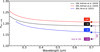 |
Fig. 1 Comparison between nuv-vis values derived by Kofman et al. (2019) and He et al. (2022). The refractive index values at 0.7 µm are indicated in the figure. The purple circle and box show the nuv-vis from Kofman et al. (2019) at 10 K reduced by 5%. |
Input parameters used to calculate the mid-IR water ice refractive index (2–20 µm).
2.3 Joining UV–vis and mid-IR data
The data described in Sects. 2.1 and 2.2 cover two spectral ranges; 0.3–0.7 µm and 2–20 µm. Clearly, for the interval between 0.7 and 2 µm, experimental spectra are not available. To cover this range the two data sets need to be linked, and we used different approaches for n and k. For k values, we extrapolated the imaginary refractive index at 2 µm (10−4) until 0.3 µm. In the case of n, we used a low-order polynomial to link the water ice n values from He et al. (2022) to the data starting at 2 µm. The caveat in this approach is that we have to neglect the water ice absorption bands in the interval between 0.7 and 2 µm. In this range, water ice has overtone transitions between 1.4 and 1.8 µm, but they are weak, both for amorphous and crystalline ice (Mastrapa et al. 2008). For example, the k values calculated by Mastrapa et al. (2008) range from 10−5 to 10−3, which covers the value used in our extrapolation (10−4). Similarly, the variation in n is rather small.
2.4 CRI values at 160 K
In addition to the CRI values of amorphous water ice taken from LIDA and shown in Sect. 2.2, we added in this paper the CRI values for crystalline ice following the steps described in Sects. 2.1–2.3. For this, we used the infrared spectrum of crystalline H2O ice (T = 160 K) measured by Gerakines et al. (1996), which followed the same experimental method described in Sect. 2. Table 1 lists the parameters used in the calculations.
2.5 UV-to-mid-IR refractive index: 0.3–20 µm
In Figs. 2a,b we show, respectively, the real and imaginary refractive index of pure amorphous water ice ranging from 0.3 to 20 µm at 30 K. We compare our results with previous data from Hudgins et al. (1993) at 40 K and from Mastrapa et al. (2009) at 25 K. Four water bands are indicated in panel b, which correspond to the symmetric and asymmetric O–H stretching mode at 3 µm (v1 and v3), the bending mode at 6 µm (v2), and the libration mode, also known as hindered rotation, at 13 µm (vL). The band at 4.5 µm is due to the combination of the bending and libration modes (v2 + vL). For the 30 K measurements presented here, a larger spectral coverage is achieved because of the used broadband method. This ensures more accuracy when deriving physical parameters depending on the refractive index.
To derive the CRI values of water ice at 30 K, we used n700nm = 1.16 from He et al. (2022), which is labelled as NK1 in Fig. 2a. For comparison with the literature values, we performed the same calculation, by assuming n700nm = 1.32 as adopted by Hudgins et al. (1993). Next, we shifted up the UV–vis data at 30 K to account for the difference in the n700nm value. The n and k values calculated from this second approach are labelled as NK2. As one can note, the NK2 CRI values are similar to what is derived by Hudgins et al. (1993), which shows that our numerical approach is consistent with Hudgins et al. (1993). The difference between NK1 and NK2 values is 13%. This difference is lower if compared to Mastrapa et al. (2009), which adopted n700nm = 1.29 taken from Dohnálek et al. (2003), measured at 22 K and assuming compact ice. In Fig. 2b, we show the k values. There is a better agreement between the band shapes derived in the present paper and Hudgins et al. (1993). However, a small difference (~7%) is seen in the peak intensity at 13 µm. The major differences in the peak intensities are observed in the spectrum from Mastrapa et al. (2009), and the water libration band is also broader. One can also note that the differences in the n values do not necessarily imply larger differences in the k values as also pointed out by Mastrapa et al. (2008). They show that the k values are much less sensitive to the n0 values, which is also observed here.
Figure 3 shows the real and imaginary parts of the H2O ice at temperatures of 30, 75, 105, and 135 K taken from LIDA and at 160 K derived in this work. The vertical offset in the real refractive indexes displayed in Fig. 3a is due to the different n700nm values used in the calculations (see Table 1). Furthermore, one can note differences in the band intensities of the imaginary refractive index at 3 µm and ~12 µm (Fig. 3b) and a blueshift of the bands for increasing temperatures. Figures 3c–h show details of the n and k profiles in selected spectral ranges. The sharpening of the 3 µm band and the increasing intensity observed in Fig. 3c for increasing temperatures is due to the structured ordering of the ice moving from amorphous to a crystalline structure. During heating, the strength of the H-bond network increases through molecular alignment in the ice, and the O–O separation between two water molecules decreases (Hagen et al. 1981). This feature also changes the n profile shown in Fig. 3d. The band at 6 µm (Fig. 3e) also provides information about the structure of the H2O ice, namely, the spectral profile is flatter at higher temperatures (>75 K) and narrower at lower temperatures (Hagen & Tielens 1982). Nevertheless, this band shape variation is not strong in the real refractive indexes (Fig. 3f). The H2O ice libration band shape and intensity are also sensitive to the temperature variation, which affects the k and n values shown in Figs. 3g,h, respectively.
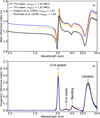 |
Fig. 2 Wavelength-dependent refractive index of H2O ice. Panels a and b show the real and imaginary parts of the complex refractive index derived in this paper (H2O at 30 K) adopting n700nm = 1.16 (black) and n700nm = 1.32 (blue) compared to literature values from Hudgins et al. (1993) given by the purple line (H2O at 40 K), and from Mastrapa et al. (2009), shown by the orange line (H2O at 25 K). The inset in panel b displays an illustration of the water vibrational modes and their corresponding motion, except the O–H combination mode at 4.5 µm. Each mode is indicated at the top of the bands. |
3 Methodology
3.1 Absorption and scattering opacities of H2O ice-coated grains
The new H2O refractive index at 30 K presented here differs from previous values in the literature that assumed high n values from experiments performed at high temperatures. Consequently, it is worth quantifying its impact on the derivation of ice-coated grain opacities. To perform this quantification, we constructed dust models assuming different geometries, for instance, perfect spheres (Mie theory; Mie 1908), hollow spheres (distribution of hollow spheres – DHS; Min et al. 2005), and ellipsoidal grains (continuous distribution of ellipsoids – CDE; Bohren & Huffman 1983). While the Mie and DHS approaches cover a large grain size distribution, the CDE equations offer an approximation in the Rayleigh limit, for example, when the grain size is much smaller than the wavelength. We also assessed the differences between those three geometries and for compact and porous ice.
These calculations are performed using optool, an open-source code dedicated to producing complex dust particle opacities (Dominik et al. 2021). In this study, the grain core composition is the same in all cases: amorphous pyroxene (Mg0.7Fe0.3SiO3; Dorschner et al. 1995) and amorphous carbon (Preibisch et al. 1993). The ice mantle is composed of pure water ice, and we adopted a wide grain size distribution, ranging from small to large grains, which is a fair approximation to study interstellar and circumstellar ice analogues. The parameters used in optool to derive the opacities are shown in Table 2. The absorption and scattering opacities are given by
 (4a)
(4a)
 (4b)
(4b)
where Cabs and Csca are the absorption and scattering cross sections, V is the volume, and ρ is the density of the icy grain. The cross-section is model-dependent, which comes with different values for different grain geometries, sizes (s) and mass fraction (mfrac) of silicate, carbon, and ice.
For small grains compared to the wavelength, also called the Rayleigh regime, the cross sections are proportional to the polar-isability αj of spheres and ellipsoids, for example, Cabs ∝ Im(αj) and Csca ∝ |αj|2. The index j represents one of the major axes of the spheroid. Here, the polarisability is given by
 (5)
(5)
where Lj is called the depolarisation factor and represents the dependence on particle shape. For a sphere, Lx = Ly = Lz = 1/3. Similarly, in other geometries such as oblate and prolate spheres, discs, and rods, these numbers change and must satisfy the condition ΣjLj = 1. The term m̃av in Eq. (5) is the combined CRI value of ice and dust, and it shows the dependence of the icy grain cross-section with the CRI values. Optool adds the ice mantle to the core by using the Maxwell-Garnett effective medium theory Garnett (1904, 1906), and m̃av is calculated by
![Mathematical equation: $\tilde m_{{\rm{av}}}^2 = \tilde m_{{\rm{core }}}^2\left[ {1 + {{3f\left( {\tilde m_{{\rm{mantle }}}^2 - \tilde m_{{\rm{core }}}^2} \right)/\left( {\tilde m_{{\rm{mantle }}}^2 + \tilde m_{{\rm{core }}}^2} \right)} \over {1 - f\left( {\tilde m_{{\rm{mantle }}}^2 - \tilde m_{{\rm{core }}}^2} \right)/\left( {\tilde m_{{\rm{mantle }}}^2 + \tilde m_{{\rm{core }}}^2} \right)}}} \right],$](/articles/aa/full_html/2024/01/aa47437-23/aa47437-23-eq15.png) (6)
(6)
where m̃core and m̃mantle are the CRI values for the dust grain and the ice mantle, respectively; f is the volume fraction of the ice inclusions. The effect of the ice porosity is calculated by the following equation obtained by
 (7)
(7)
(Hage & Greenberg 1990), where P is the porosity factor ranging from 0 (i.e. compact icy grain) to 1 − δ (i.e. porous icy grain), and δ ≪ 1. When the ice porosity is considered in the models,  replaces
  in Eq. (6).
For particles of the same size as the wavelength, the cross-sections become a function of Legendre polynomials and Bessel functions (Mie 1908; Bohren & Huffman 1983). The physical meaning is that when a plane electromagnetic wave interacts with a homogeneous sphere in a vacuum, it causes the sphere to produce a non-isotropic outgoing wave. This wave can be expanded using spherical harmonics. For completeness, we quote the cross-sections from Bohren & Huffman (1983):
 (8a)
(8a)
 (8b)
(8b)
 (8c)
(8c)
where v = 2π/λ is the wave number of the incoming wave, j is the expansion index, and aj and bj are called scattering coefficients, which are a function of m̃. Evidently, when particles are smaller than the involved wavelength, the Mie theory produces cross-sections as the Rayleigh approach. In the case of particles that are large compared to the wavelength – the geometric-optics limit – the same formalism is used, and the calculations become significantly more expensive.
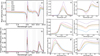 |
Fig. 3 Wavelength-dependent refractive index of H2O ice at different temperatures. Panels a and b show the real and imaginary parts of the complex refractive index in a broad-range perspective (0.3–20 µm). Panels c–h show zoomed-in images of selected wavelengths in panels a and b indicated by the hatched areas. |
Input parameters used to calculate the absorption and scattering opacities.
3.2 Radiative transfer calculations
To fully assess the impact of the icy grain opacities resulting from the new CRI values, we ran three-dimensional radiative transfer calculations to calculate the spectral energy distribution (SED) of a star surrounded by icy grains. As a proof of concept, we adopted the water ice CRI values at 30 K. The goal of this approach is to assess the differences in the SED by using different ice-dust opacities introduced in Sect. 3.1. The simulations are carried out by using the radiative transfer code RADMC-3D (Dullemond et al. 2012). We adopted an axisymmetric density structure and performed a full three-dimensional simulation where we kept the source inclinations at 80°.
Our simplified model assumes that a forming star is surrounded by a spherical envelope with no disc inside. The envelope density profile at different radii (r) is the same as that used in previous works (e.g. Pontoppidan et al. 2005; Rocha & Pilling 2015) and is given by
 (9)
(9)
where Rout is the outer envelope radius. Table 3 summarises the parameters used in this model.
4 Results
4.1 Ice-grain opacities
In this section, we compare the opacity values derived from the NK1 and NK2 refractive indexes, which are those using n700nm = 1.16 and n700nm = 1.32, respectively. No comparisons are made with Hudgins et al. (1993) and Mastrapa et al. (2009) because of different experimental settings, such as the ice growth rate and chamber pressure, which relate to the presence of background gas contaminants that may induce systematic effects. Additionally, NK1 and NK2 values cover a broader spectral range compared to the literature. In this sense, the comparison of values derived from the same experimental data offers a more consistent approach.
Figure 4 shows the absorption and scattering opacities of spherical grains in the framework of the Mie theory and when compact and porous ices are adopted. The differences between the opacity values calculated from NK1 and NK2 are also shown at the bottom of each panel and are calculated using
 (10)
(10)
where κNK1 and κNK2 are the opacities derived by assuming n700nm = 1.16 and n700nm = 1.32, respectively. Quantitatively, the ∆ĸabs,sca values in Figs. 4a,b show that the absorption opacity calculated from NK1 values reduces the opacity baseline by 3–5% when compared to the opacities derived from NK2 refractive indexes. Furthermore, it leads to slightly more absorption (4–5%) at wavelengths around ~3 µm and ~12 µm, where the O–H stretching and the libration bands are located, respectively. Another interesting aspect of using the NK1 values is the increase of absorption opacity around 11.6 µm, where the H2O libration band is located. Compact ice enhances this feature by 5% compared to 2.8% in porous ice. The new refractive indexes derived for NK1 also affect the scattering opacities. Figures 4c,d show a reduction in the scattering of around 8% in most of the wavelengths, and around 13% at 3 µm independently whether the ice is compact or porous.
Figure 5 shows zoomed-in views between the 7.5 and 15 µm of Fig. 4. At 11.6 µm, we observe the presence of the H2O libra-tion band when the NK1 values are used to calculate absorption and scattering opacities. This feature is more prominent when the ice is compact and weaker in porous ice. If NK2 refractive indexes are used, this feature becomes weaker or is no longer visible.
In Fig. 6, we investigated the differences in the opacities for both compact and porous grains when the DHS model is considered. The absorption and scattering opacities shown in panels a–d have a similar trend compared to the Mie ice-dust models (Fig. 4). There is an increase in the absorption opacity of 3–5% around 3 µm and 12 µm. Additionally, the bump around 11.6 µm associated with the H2O libration band is also present in the model of compact ices. Conversely, this band is hidden when NK2 values are adopted to derive the opacities or when the ice is porous. Again, the most notable effect of using NK1 values is seen in the scattering opacities. Specifically, around 3 µm and 12 µm, the scattering is reduced by around 15% and 10%, respectively.
Finally, in Fig. 7, we assessed the impact of the new H2O ice refractive index on grains modelled using the CDE approach, for example, assuming grains with ellipsoidal shapes. First, we note the increase in the absorption opacity around 3 µm and 12 µm of ~12%, which is two times higher than in the Mie and DHS models. Second, the H2O libration band is a persistent feature in compact ices when NK1 refractive indexes are used. As in the other cases, it becomes weaker again when the ice is porous or when the NK2 values are considered. Moreover, the NK1 values have a substantial impact on the scattering opacity. Specifically, it is reduced by as much as 28–34% at 3 µm.
The differences in the absorption and scattering opacities around 3 µm shown in Figs. 4–7 are summarised in Fig. 8. We note that (i) there are more significant differences in the opacities when the ice is compact, (ii) opacity differences in CDE models are more prominent than in Mie and DHS models, (iii) the new H2O ice refractive index reduces by more than 25% the scattering opacity in CDE models, (iv) the differences between Mie and DHS models are comparable. This highlights the need for accurate refractive indexes of the most abundant molecules in ice when using them to derive opacities for spectral data interpretation.
Input parameters used to calculate the mid-IR water ice refractive index.
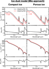 |
Fig. 4 Absorption (upper panels) and scattering (lower panels) opacities of ice-dust grains assuming compact (left) and porous ices (right). Lines in black are the opacities assuming the water ice refractive index derived in this paper, for instance, assuming n700nm = 1.16 (NK1), whereas red curves show the opacities calculated using n700nm = 1.32 (NK2). The small panels below the large ones show the variation between the two opacities in percentage values. A small offset is performed on the absorption opacities for better readability. No offset is applied to the scattering opacity. Zoomed-in images of the rectangular regions indicated by the grey dotted boxes are provided in Fig. 5. |
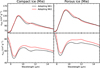 |
Fig. 5 Zoomed-in view of the absorption and scattering opacities of icedust grains shown in Fig. 4. The left and right panels show the opacities assuming compact and porous ice grains. No offset is applied in this absorption opacity. |
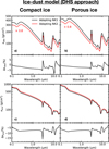 |
Fig. 6 Same as Fig. 4, but assuming the DHS approach. An offset on the absorption opacity is used for better readability. No offset is applied on the scattering opacity. |
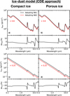 |
Fig. 7 Same as Fig. 4, but assuming the CDE approach. An offset on both absorption and scattering opacities is applied for better readability. |
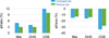 |
Fig. 8 Bar plot showing percentage difference between absorption (left) and scattering (right) opacities calculated from NK1 and NK2 values for compact (blue) and porous ice (violet). The bars are grouped by the method adopted to calculate opacities, for instance, Mie, DHS, and CDE. Positive and negative values indicate an increase and decrease in the opacity value, respectively. |
4.2 Protostellar spectrum and H2O ice column density
In order to make the previous findings more concrete, we ran radiative transfer models using the RADMC-3D code to compute the effect of the ice opacities in the spectrum of a protostar surrounded by an envelope. Specifically, we used opacities derived from models M1c, M1p, M2c, and M2p (see Table 3) under the DHS and CDE approaches. Figures 9a,b show the mid-IR spectrum of grains under the DHS approach. In models Mlc and Mlp, silicate and all H2O ice bands are seen, including the bump around the water ice libration mode at 11.6 µm. In models M2c and M2p, the absorption excess at 11.6 µm is not visible in the synthetic spectra, as indicated by the opacity values.
The water ice bands have different absorption intensities in models M1c and M1p. We used these synthetic protostellar spectra to assess the impact of the NK1 and NK2 values on the determination of the H2O ice column density. Figures 9c,d compare the optical depth spectrum of the H2O ice band at 3 µm in both cases. To convert the spectrum from flux to optical depth scale, we used the equation  , where
  is the protostellar flux and
  is the continuum flux. The continuum is determined by a low-order polynomial function. We note that the NK1 refractive index values lead to more light extinction at 3 µm both when the ice is porous and compact (Models M1p and M1c), compared to the models considering the NK2 values (M2p and M2c). Moreover, they result in slightly more absorption if the ice is compact instead of porous.
Finally, we derived the H2O ice column densities from the O–H stretching mode at 3 µm. Figures 9e,f display bar plots to compare the differences between the ice column densities. These are calculated with the equation  , where A is the band strength of the O–H stretching mode, equal to 2 × 10⁻¹⁶ cm molecule−1 (Gerakines et al. 1995). We can see from Fig. 9e that if the ices are compact, the column density is 10% higher for NK1 values compared to NK2 values. Figure 9f shows that if the ices are porous, the difference between column densities is around 6%. This again highlights the fact that in order to interpret astrophysical observables, such as column densities, precise refractive index values are an absolute prerequisite.
We repeated this analysis on the protostar synthetic spectra when the opacity values were derived from the CDE models, and the result is shown in Fig. 10. We note that the differences in the water ice column densities are bigger. In the case of compact grains, the H2O ice column density is 16% higher than in the cases where NK2 values are used.
5 Discussion
We have shown that the NK1 and NK2 refractive index values impact the derivation of physical parameters such as the scattering and absorption opacities, and the ice column density derivation from radiative transfer models. Now, we discuss how these results may be affected by different initial conditions, such as the effect of porosity, ice mass, and grain size on the astrophysical observables.
5.1 H2O ice libration band and ice mass
The persistent presence of the H2O libration band in compact ice models using Mie, CDE, and DHS approaches shows that this feature is independent of the dust geometry assumed to derive the opacities. It is, rather, associated with the amount of ice (ice mass) adopted in the models, which is given as a percentage relative to the total dust core mass. In Fig. 11, we explored how the relative intensity of the band at 11.6 µm changes as a function of the ice porosity and mass. The relative intensity refers to the opacity value after local baseline subtraction around 11.6 µm. The porosity and ice mass vary from 0 to 25%. From this figure, we find that the highest intensity (light yellow colour) is when the ice is compact (no porosity) and the ice mass is 25% of the total dust mass. The dark blue colour indicates the lowest relative intensity. It should be noted that this figure does not constrain the detection limit to observe the 11.6 µm by itself since this depends on the protostar and the sensitivity of the instruments used in the observations.
In Fig. 12a, we show various protostar synthetic spectra in optical depth scale between 7 and 15 µm where we assume compact and porous ice and the ice mass varying from 5 to 25%. These spectra are normalized by the optical depth at 9 µm. It is clear that the peak at 11.6 µm increases with the ice mass. The profile at 11.6 µm is often more intense in models with compact ice than when the ice is porous. Additionally, we compare these envelope models with the spectra of the low-mass protostar, HH 46. This protostar shows a prominent band around 9.7 µm, likely related to the absorption of methanol ice, which is not considered in the models. In Fig. 12b, we perform a comparison of the 11.6 µm profile of HH 46 with four selected parameter settings, namely, compact and porous ice with ice mass of 15% and 25% in each case. This comparison is carried out after local baseline subtraction to reduce the effect of the silicate absorption feature. This shows that porous ice with an ice mass of 15% matches better than the other models. Boogert et al. (2008) showed that this band is, in fact, associated with the H2O ice libration band which is aligned with our result. Our models do not fit the 11.2 µm, which is likely related to the presence of crystalline silicates (e.g., Kessler-Silacci et al. 2005; Do-Duy et al. 2020).
Figure 13 shows additional data that suggest the presence of porous water ice towards high-mass protostars. The absorption profile around 11 µm is taken from Do-Duy et al. (2020), which is obtained after local baseline subtraction. An asymmetric Gaussian profile was used to fit the crystalline silicate feature. Towards two high-mass sources, MonR2 IRS2 and AFGL 989, there is an absorption excess at 11.6 µm that is not fitted with the Gaussian profile. However, this band shows a good match with the scaled H2O ice libration band obtained from the simulated protostar spectrum considering an ice mass of 15% and porous structure, which is similar to HH46 (see Fig. 12). The two protostars are known to have H2O ice detected at 3 and 6 µm (Gibb et al. 2004), which further supports the presence of water ice at 11.6 µm. Conversely, GCS3 does not have H2O ice detection associated with it, and its silicate profile is often used as a template to remove the silicate features towards other protostars (e.g. Boogert et al. 2008; Bottinelli et al. 2010; Rocha et al. 2021). In fact, no water ice profile is suggested from this comparison.
Typically, laboratory studies consider the OH dangling bond of H2O ice at 2.7 µm as a tracer of the ice porosity (e.g. McCoustra & Williams 1996; Palumbo 2005; Nagasawa et al. 2021), although the absence of this band is not proof the ice is fully compact (Isokoski et al. 2014; Bossa et al. 2015). Until now, the OH dangling bond had only tentatively been observed in the background star NIR38 with JWST under the Ice Age ERS programme (McClure et al. 2023). Earlier astronomical observations were unable to detect this band, likely because of limitations in instrumental sensitivity. Moreover, the intensity of the OH dangling mode in the near-IR range may be severely reduced due to the circumstellar dust extinction.
In addition to the OH dangling bond, the comparisons shown in Figs. 12 and 13 indicate that the H2O libration band profile can be used as a diagnostic of the ice porosity in protostellar environments as well. In this regard, we encourage further work around the silicate feature at 9.8 µm to constraints on the ice structure. Specifically, low-mass protostars are ideal targets to be observed with the JWST, and the sensitivity of the Mid-Infrared Instrument (MIRI) allows the achievement of this goal.
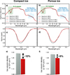 |
Fig. 9 Effects of opacity values derived for grains under DHS approach by assuming NK1 and NK2 values. Panel a shows the synthetic protostellar spectrum with H2O ice and silicate absorption bands calculated from opacity models based on NK1 (black) and NK2 (red) refractive index values. The black and red and dashed lines over the 3 µm feature are the continuum. The blue box around 13 µm highlights the absence of the H2O libration band in the spectrum derived from NK2 values. Panel b displays the same as panel a but for porous ice. Panels c and d present the H2O ice column density derived from the optical depth spectrum using compact and porous ices, respectively. Finally, panels e and f compare the ice column densities from both cases (grey: NK1; red: NK2). |
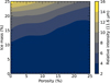 |
Fig. 11 Relative intensity of 11.6 µm profile by assuming different ice mass and porosity. |
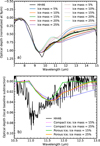 |
Fig. 12 Comparisons between icy-dust models with an astronomical observation. (a) Normalised synthetic spectra in optical depth scale of models assuming compact (coloured dotted lines) and porous (coloured solid lines) ice and different ice mass. The spectrum of HH 46 is shown in black for comparison. The vertical grey line indicates the profile at 11.6 µm. (b) Comparison between the observed profile around 11.6 µm in HH 46 with four synthetic spectra after local baseline subtraction. The synthetic spectra are derived using two ice masses (15% and 25% relative to dust mass) for compact and porous ice. |
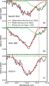 |
Fig. 13 Comparison between absorption feature around 11 µm observed towards different sources with H2O ice libration band from synthetic spectra. Panels a–c show in black the profiles for the highmass protostars Monoceros R2-IRS, AFGL 989, and the galactic centre source GCS3 II, respectively. The dashed red line is an asymmetric Gaussian fit of the 11.2 µm performed by Do-Duy et al. (2020). The solid green line is the profile of the H2O ice libration band from a model assuming an ice mass of 15% distributed in porous ice and scaled to the peak optical depth at 11.6 µm, which is indicated by the vertical grey line. |
5.2 How big are the grains to hide the H2O ice feature in the mid-IR?
The improved H2O ice CRI values derived from this work also extend the discussion on how the size of the grains affects the strength of the water ice absorptions at 3 and 6 µm. Based on the study of water ice in the coma of comet Hale-Bopp, Lellouch et al. (1998) estimated a mean icy grain size of 15 µm to hide the IR water ice feature at 3 µm. However, the authors indicated that their assumption of a single-grain size is not realistic for sublimating icy grains. Additional work by van Dishoeck et al. (2021) calculated a grain size threshold of 10 µm for the detection of the 3 µm band.
In Fig. 14, we showed the changes in the optical depth at 3 and 6 µm when the grain size increases and different porosity levels are taken into account. For these calculations, we chose the DHS approach that simulates irregular grain shapes and we keep an ice mass of 25% constant. For compact ices shown in panels a and b, increasing the grain size from agrain = 0.1 µm to agrain = 1 µm reduces the ice column density by ~33%. This reduction is more significant – by a factor of 8 when the grain grows to agrain = 10 µm. For porous ices, the reduction in the column density is 30% and a factor of 4 if the grain grows from 0.1 µm to 1 µm and 10 µm, respectively. Notably, the difference is lower when the ice is porous. We performed the same analysis on the 6 µm band, shown in panels c and d. The ice column density decreases by 40% and 92% when the icy grain grows from 0.1 µm to 1 µm and from 0.1 µm to 10 µm, respectively. When the ice is porous, the reduction is 35% and 80%, respectively.
Based on the variations in the intensities of the H2O ice bands with grain size, we explored the combined effect of grain growth and ice mass and porosity variation. In Fig. 15, we showed a contour map of absorption opacities at 3 µm (left) and 6 µm (right) by changing porosity and ice mass. The blue hatched area indicates an optical depth below 0.01, where the ice band is no longer observable. At 3 µm, the O–H stretching mode can be detected for grains with sizes from 13 µm to 18 µm, depending on the ice mass and porosity. This occurs because the ice mass is kept constant when the size of the grain increases. Therefore, the amount of ice distributed on the grain surface decreases (see Eqs. (4a) and (4b)). We performed the same analysis of the H2O bending mode at 6 µm. The minimum grain size threshold is around 16–17 µm, but this water feature in grains larger than 20 µm remains observable because the opacity is lower at this wavelength.
An interesting side effect of the work discussed here is that this analysis may also help to further constrain the problem of the missing oxygen, for instance, the lower oxygen budget in star-forming regions compared with diffuse clouds. An elegant solution proposed for cold protostar envelopes is that large grains suppress H2O ice features, which are not observable. In our analysis, grains need to grow larger than 10 µm and 15 µm to suppress the 3 µm and 6 µm water bands, respectively. Although it remains a challenge to explain grain growth at the millimetre level via a coagulation process (e.g., Silsbee et al. 2022), there are sufficient observational studies showing that µm-size grains are rather plausible in dense clouds (e.g. Pagani et al. 2010; Miotello et al. 2014; Dartois et al. 2022). It is important to highlight that there are other oxygen-bearing molecules hosting a large amount of oxygen in the solid phase, and that are not easily visible in the infrared spectrum. For example, molecular oxygen (O2), has not been detected yet in interstellar ices. New experimental works have explored this problem further and provided laboratory data to search for O2 in ices (Müller et al. 2022).
We note that pure H2O ice does not exist in space; it is typically mixed with other hydrogenated species (e.g. NH3, CH4; Dartois & d’Hendecourt 2001; Öberg et al. 2008; Qasim et al. 2018), as well as with CO, CO2, CH3OH (Gerakines et al. 1999; Pontoppidan et al. 2008; McClure et al. 2023) after the CO freeze-out. Nevertheless, Isokoski et al. (2014) show that the real refractive index at 632.8 nm of the H2O:CO2 ice mixture at 20 K is 1.22 for a CO2 ice fraction of 10% and 1.24 for a fraction of 20%. These numbers are around 5% higher than the n700nm used in this paper for the pure H2O ice, but still 10% lower than the typical value used in the literature (1.32). Despite this caveat, the numbers discussed here definitely will be useful for studying low-temperature environments dominated by water ice. In the near future, new work will provide temperature and wavelength-dependent CRI values for ice mixtures to improve on recording data of astrophysical relevance, as well as to further explore the role of the ice mixtures in the interpretation of ice observations.
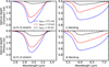 |
Fig. 14 Optical depth variation with grain growth and ice porosity. Panels a and b show the changes for the O–H stretching mode, and panels c and d show the H2O ice bending mode. We note the different vertical scales for the two wavelength regimes. |
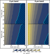 |
Fig. 15 Absorption opacity map of 3 µm (left) and 6 µm (left) water ice bands for different grain sizes, ice porosity, and ice masses. The blue hatched area indicates the region where the H2O ice modes are no longer detectable. |
6 Conclusions
We show how broad-band complex refractive index values recently derived using a new technique impact astrophysical observables such as ice column density and grain size. For this, we studied the UV-to-mid-IR complex refractive index of H2O ice in detail for a large range of temperatures: 30, 75, 105, 135, and 160 K. Below 160 K, the CRI values are lower than previously estimated in the literature. At 30 K, the real refractive index is around 14% lower. Below, we summarise the main conclusions of this work:
The new refractive index values of H2O ice-covered grains lead to more absorption and less scattering for the 3 µm band. Quantitatively, this difference is due to the grain model adopted and whether the ice is porous or compact. Under Mie and DHS approaches, the values are similar and range from 3–5% more absorption and 15% less scattering. Under the CDE approach, there is around 10–12% more absorption and 28–35% less scattering;
Ice column densities derived from simulated spectra using the new and previous refractive indexes are different. Under the CDE approach, the H2O ice column density derived from the 3 µm band is 16% and 8% higher if the ice is compact and porous, respectively. Under the DHS approach, the differences are 10% and 6%, respectively;
Adopting the new refractive index values to derive grain opacities suggests that the H2O has a prominent feature at 11.6 µm, which is not visible when previous refractive indexes are used. The shape of this band changes with the ice porosity level. We find that when this band is associated with a porosity level of 15%, it can explain the absorption excess observed towards the low-mass protostar HH 46 and the high-mass protostars MonR2 IRS2 and AFGL 989. Therefore, in addition to the OH dangling mode at 2.7 µm, the water libration band offers an additional spectral range to constrain the porosity level of interstellar ices;
The grain size threshold to detect the 3 µm feature is pushed further in this work to 18 µm and depends on the ice mass and porosity. Likewise, the 6 µm band remains detectable even for grains larger than 20 µm.
An accurate determination of the physico-chemical properties of H2O ice is key for a better interpretation of astronomical observations. This definitely applies for ongoing JWST work, but also will be relevant for future space missions, visiting icy bodies in our Solar System.
Acknowledgements
We thank the referee, James Stubbing, for the constructive comments that improved the quality and clarity of this manuscript. This project has received funding from the European Research Council (ERC) under the European Union’s Horizon 2020 research and innovation programme (grant agreement no. 291141 MOLDISK). This work is supported by the Danish National Research Foundation through the Center of Excellence “InterCat” (Grant agreement no.: DNRF150), and by the Netherlands Research School for Astronomy (NOVA), grant 618.000.001. W.R.M.R. also thanks Ardjan Sturm for stimulating discussions, Carsten Domenik for making the Optool code publicly available. This research has made use of NASA’s Astrophysics Data System Bibliographic Services (ADS). This research builds upon the work originally started by Vincent Kofman on the measurements of H2O ice refractive index in the UV-vis range conducted at the Laboratory for Astrophysics in Leiden. Here it is extended beyond their original objectives.
References
- Bell, J. F. 2010, Highlights Astron., 15, 29 [NASA ADS] [Google Scholar]
- Beuther, H., van Dishoeck, E. F., Tychoniec, L., et al. 2023, A&A, 673, A121 [NASA ADS] [CrossRef] [EDP Sciences] [Google Scholar]
- Bohren, C. F., & Huffman, D. R. 1983, Absorption and Scattering of Light by Small Particles (New York: Wiley) [Google Scholar]
- Boogert, A. C. A., Pontoppidan, K. M., Knez, C., et al. 2008, ApJ, 678, 985 [Google Scholar]
- Boogert, A. C. A., Gerakines, P. A., & Whittet, D. C. B. 2015, ARA&A, 53, 541 [Google Scholar]
- Bossa, J.-B., Maté, B., Fransen, C., et al. 2015, ApJ, 814, 47 [NASA ADS] [CrossRef] [Google Scholar]
- Bottinelli, S., Boogert, A. C. A., Bouwman, J., et al. 2010, ApJ, 718, 1100 [NASA ADS] [CrossRef] [Google Scholar]
- Chu, L. E. U., Hodapp, K., & Boogert, A. 2020, ApJ, 904, 86 [NASA ADS] [CrossRef] [Google Scholar]
- Dartois, E., & d’Hendecourt, L. 2001, A&A, 365, 144 [NASA ADS] [CrossRef] [EDP Sciences] [Google Scholar]
- Dartois, E., Noble, J. A., Ysard, N., Demyk, K., & Chabot, M. 2022, A&A, 666, A153 [NASA ADS] [CrossRef] [EDP Sciences] [Google Scholar]
- Do-Duy, T., Wright, C. M., Fujiyoshi, T., et al. 2020, MNRAS, 493, 4463 [Google Scholar]
- Dohnálek, Z., Kimmel, G. A., Ayotte, P., Smith, R. S., & Kay, B. D. 2003, J. Chem. Phys., 118, 364 [CrossRef] [Google Scholar]
- Dominik, C., Min, M., & Tazaki, R. 2021, OpTool: Command-line driven tool for creating complex dust opacities, Astrophysics Source Code Library, [record ascl:2104.010] [Google Scholar]
- Dorschner, J., Begemann, B., Henning, T., Jaeger, C., & Mutschke, H. 1995, A&A, 300, 503 [Google Scholar]
- Dullemond, C. P., Juhasz, A., Pohl, A., et al. 2012, RADMC-3D: a multipurpose radiative transfer tool, Astrophysics Source Code Library [record ascl:1202.015] [Google Scholar]
- Encrenaz, T. 2008, ARA&A, 46, 57 [NASA ADS] [CrossRef] [Google Scholar]
- Garnett, J. C. M. 1904, Philos. Trans. Roy. Soc. Lond. A, 203, 385 [NASA ADS] [CrossRef] [Google Scholar]
- Garnett, J. C. M. 1906, Philos. Trans. Roy. Soc. Lond. A, 205, 237 [NASA ADS] [CrossRef] [Google Scholar]
- Gerakines, P. A., & Hudson, R. L. 2020, ApJ, 901, 52 [NASA ADS] [CrossRef] [Google Scholar]
- Gerakines, P. A., Schutte, W. A., Greenberg, J. M., & van Dishoeck, E. F. 1995, A&A, 296, 810 [NASA ADS] [Google Scholar]
- Gerakines, P. A., Schutte, W. A., & Ehrenfreund, P. 1996, A&A, 312, 289 [NASA ADS] [Google Scholar]
- Gerakines, P. A., Whittet, D. C. B., Ehrenfreund, P., et al. 1999, ApJ, 522, 357 [NASA ADS] [CrossRef] [Google Scholar]
- Gibb, E. L., Whittet, D. C. B., Schutte, W. A., et al. 2000, ApJ, 536, 347 [Google Scholar]
- Gibb, E. L., Whittet, D. C. B., Boogert, A. C. A., & Tielens, A. G. G. M. 2004, ApJS, 151, 35 [NASA ADS] [CrossRef] [Google Scholar]
- Gillett, F. C., & Forrest, W. J. 1973, ApJ, 179, 483 [NASA ADS] [CrossRef] [Google Scholar]
- Hage, J. I., & Greenberg, J. M. 1990, ApJ, 361, 251 [NASA ADS] [CrossRef] [Google Scholar]
- Hagen, W., & Tielens, A. G. G. M. 1982, Spectrochim. Acta A: Mol. Spectrosc., 38, 1089 [NASA ADS] [CrossRef] [Google Scholar]
- Hagen, W., Tielens, A. G. G. M., & Greenberg, J. M. 1981, Chem. Phys., 56, 367 [NASA ADS] [CrossRef] [Google Scholar]
- Hale, G. M., & Querry, M. R. 1973, Appl. Opt., 12, 555 [NASA ADS] [CrossRef] [Google Scholar]
- He, J., Diamant, S. J. M., Wang, S., et al. 2022, ApJ, 925, 179 [NASA ADS] [CrossRef] [Google Scholar]
- Hudgins, D. M., Sandford, S. A., Allamandola, L. J., & Tielens, A. G. G. M. 1993, ApJS, 86, 713 [NASA ADS] [CrossRef] [Google Scholar]
- Irvine, W. M., & Pollack, J. B. 1968, Icarus, 8, 324 [NASA ADS] [CrossRef] [Google Scholar]
- Isokoski, K., Bossa, J. B., Triemstra, T., & Linnartz, H. 2014, Phys. Chem. Chem. Phys. (Incorp. Faraday Trans.), 16, 3456 [NASA ADS] [CrossRef] [Google Scholar]
- Kessler-Silacci, J. E., Hillenbrand, L. A., Blake, G. A., & Meyer, M. R. 2005, ApJ, 622, 404 [Google Scholar]
- Kofman, V., He, J., Loes ten Kate, I., & Linnartz, H. 2019, ApJ, 875, 131 [NASA ADS] [CrossRef] [Google Scholar]
- Lellouch, E., Crovisier, J., Lim, T., et al. 1998, A&A, 339, L9 [NASA ADS] [Google Scholar]
- Mastrapa, R. M., Bernstein, M. P., Sandford, S. A., et al. 2008, Icarus, 197, 307 [NASA ADS] [CrossRef] [Google Scholar]
- Mastrapa, R. M., Sandford, S. A., Roush, T. L., Cruikshank, D. P., & Dalle Ore, C. M. 2009, ApJ, 701, 1347 [NASA ADS] [CrossRef] [Google Scholar]
- McClure, M. K., Rocha, W. R. M., Pontoppidan, K. M., et al. 2023, Nat. Astron., 7, 431 [NASA ADS] [CrossRef] [Google Scholar]
- McCoustra, M., & Williams, D. A. 1996, MNRAS, 279, L53 [NASA ADS] [CrossRef] [Google Scholar]
- Mie, G. 1908, Ann. Phys., 330, 377 [Google Scholar]
- Min, M., Hovenier, J. W., & de Koter, A. 2005, A&A, 432, 909 [NASA ADS] [CrossRef] [EDP Sciences] [Google Scholar]
- Miotello, A., Testi, L., Lodato, G., et al. 2014, A&A, 567, A32 [NASA ADS] [CrossRef] [EDP Sciences] [Google Scholar]
- Müller, B., Giuliano, B. M., Vasyunin, A., Fedoseev, G., & Caselli, P. 2022, A&A, 668, A46 [NASA ADS] [CrossRef] [EDP Sciences] [Google Scholar]
- Nagasawa, T., Sato, R., Hasegawa, T., et al. 2021, ApJ, 923, L3 [NASA ADS] [CrossRef] [Google Scholar]
- Nna-Mvondo, D., & Anderson, C. M. 2022, ApJ, 925, 123 [NASA ADS] [CrossRef] [Google Scholar]
- Öberg, K. I., Fraser, H. J., Boogert, A. C. A., et al. 2007, A&A, 462, 1187 [NASA ADS] [CrossRef] [EDP Sciences] [Google Scholar]
- Öberg, K. I., Boogert, A. C. A., Pontoppidan, K. M., et al. 2008, ApJ, 678, 1032 [Google Scholar]
- Pagani, L., Steinacker, J., Bacmann, A., Stutz, A., & Henning, T. 2010, Science, 329, 1622 [Google Scholar]
- Palumbo, M. E. 2005, J. Phys. Conf. Ser., 6, 211 [Google Scholar]
- Pontoppidan, K. M., van Dishoeck, E. F., & Dartois, E. 2004, A&A, 426, 925 [NASA ADS] [CrossRef] [EDP Sciences] [Google Scholar]
- Pontoppidan, K. M., Dullemond, C. P., van Dishoeck, E. F., et al. 2005, ApJ, 622, 463 [NASA ADS] [CrossRef] [Google Scholar]
- Pontoppidan, K. M., Boogert, A. C. A., Fraser, H. J., et al. 2008, ApJ, 678, 1005 [NASA ADS] [CrossRef] [Google Scholar]
- Preibisch, T., Ossenkopf, V., Yorke, H. W., & Henning, T. 1993, A&A, 279, 577 [NASA ADS] [Google Scholar]
- Qasim, D., Chuang, K. J., Fedoseev, G., et al. 2018, A&A, 612, A83 [NASA ADS] [CrossRef] [EDP Sciences] [Google Scholar]
- Querry, M. R. 1987, in Optical constants of minerals and other materials from the millimeter to the ultraviolet [Google Scholar]
- Rocha, W., & Pilling, S. 2014, Spectrochim. Acta A: Mol. Biomol. Spectrosc., 123, 436 [CrossRef] [Google Scholar]
- Rocha, W. R. M., & Pilling, S. 2015, ApJ, 803, 18 [NASA ADS] [CrossRef] [Google Scholar]
- Rocha, W. R. M., Perotti, G., Kristensen, L. E., & Jørgensen, J. K. 2021, A&A, 654, A158 [NASA ADS] [CrossRef] [EDP Sciences] [Google Scholar]
- Rocha, W. R. M., Rachid, M. G., Olsthoorn, B., et al. 2022, A&A, 668, A63 [NASA ADS] [CrossRef] [EDP Sciences] [Google Scholar]
- Silsbee, K., Akimkin, V., Ivlev, A. V., et al. 2022, ApJ, 940, 188 [NASA ADS] [CrossRef] [Google Scholar]
- Snodgrass, C., Agarwal, J., Combi, M., et al. 2017, A&ARv, 25, 5 [NASA ADS] [CrossRef] [Google Scholar]
- Stubbing, J. W., McCoustra, M. R. S., & Brown, W. A. 2020, Phys. Chem. Chem. Phys. (Incorp. Faraday Trans.), 22, 25353 [NASA ADS] [CrossRef] [Google Scholar]
- van Dishoeck, E. F., Kristensen, L. E., Mottram, J. C., et al. 2021, A&A, 648, A24 [NASA ADS] [CrossRef] [EDP Sciences] [Google Scholar]
- Whittet, D. C. B., Gerakines, P. A., Hough, J. H., & Shenoy, S. S. 2001, ApJ, 547, 872 [Google Scholar]
- Yang, Y.-L., Green, J. D., Pontoppidan, K. M., et al. 2022, ApJ, 941, L13 [NASA ADS] [CrossRef] [Google Scholar]
All Tables
Input parameters used to calculate the mid-IR water ice refractive index (2–20 µm).
All Figures
|
Fig. 1 Comparison between nuv-vis values derived by Kofman et al. (2019) and He et al. (2022). The refractive index values at 0.7 µm are indicated in the figure. The purple circle and box show the nuv-vis from Kofman et al. (2019) at 10 K reduced by 5%. |
| In the text | |
|
Fig. 2 Wavelength-dependent refractive index of H2O ice. Panels a and b show the real and imaginary parts of the complex refractive index derived in this paper (H2O at 30 K) adopting n700nm = 1.16 (black) and n700nm = 1.32 (blue) compared to literature values from Hudgins et al. (1993) given by the purple line (H2O at 40 K), and from Mastrapa et al. (2009), shown by the orange line (H2O at 25 K). The inset in panel b displays an illustration of the water vibrational modes and their corresponding motion, except the O–H combination mode at 4.5 µm. Each mode is indicated at the top of the bands. |
| In the text | |
|
Fig. 3 Wavelength-dependent refractive index of H2O ice at different temperatures. Panels a and b show the real and imaginary parts of the complex refractive index in a broad-range perspective (0.3–20 µm). Panels c–h show zoomed-in images of selected wavelengths in panels a and b indicated by the hatched areas. |
| In the text | |
|
Fig. 4 Absorption (upper panels) and scattering (lower panels) opacities of ice-dust grains assuming compact (left) and porous ices (right). Lines in black are the opacities assuming the water ice refractive index derived in this paper, for instance, assuming n700nm = 1.16 (NK1), whereas red curves show the opacities calculated using n700nm = 1.32 (NK2). The small panels below the large ones show the variation between the two opacities in percentage values. A small offset is performed on the absorption opacities for better readability. No offset is applied to the scattering opacity. Zoomed-in images of the rectangular regions indicated by the grey dotted boxes are provided in Fig. 5. |
| In the text | |
|
Fig. 5 Zoomed-in view of the absorption and scattering opacities of icedust grains shown in Fig. 4. The left and right panels show the opacities assuming compact and porous ice grains. No offset is applied in this absorption opacity. |
| In the text | |
|
Fig. 6 Same as Fig. 4, but assuming the DHS approach. An offset on the absorption opacity is used for better readability. No offset is applied on the scattering opacity. |
| In the text | |
|
Fig. 7 Same as Fig. 4, but assuming the CDE approach. An offset on both absorption and scattering opacities is applied for better readability. |
| In the text | |
|
Fig. 8 Bar plot showing percentage difference between absorption (left) and scattering (right) opacities calculated from NK1 and NK2 values for compact (blue) and porous ice (violet). The bars are grouped by the method adopted to calculate opacities, for instance, Mie, DHS, and CDE. Positive and negative values indicate an increase and decrease in the opacity value, respectively. |
| In the text | |
|
Fig. 9 Effects of opacity values derived for grains under DHS approach by assuming NK1 and NK2 values. Panel a shows the synthetic protostellar spectrum with H2O ice and silicate absorption bands calculated from opacity models based on NK1 (black) and NK2 (red) refractive index values. The black and red and dashed lines over the 3 µm feature are the continuum. The blue box around 13 µm highlights the absence of the H2O libration band in the spectrum derived from NK2 values. Panel b displays the same as panel a but for porous ice. Panels c and d present the H2O ice column density derived from the optical depth spectrum using compact and porous ices, respectively. Finally, panels e and f compare the ice column densities from both cases (grey: NK1; red: NK2). |
| In the text | |
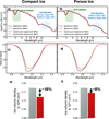 |
Fig. 10 Same as Fig. 9, but assuming icy grains under CDE approach. |
| In the text | |
|
Fig. 11 Relative intensity of 11.6 µm profile by assuming different ice mass and porosity. |
| In the text | |
|
Fig. 12 Comparisons between icy-dust models with an astronomical observation. (a) Normalised synthetic spectra in optical depth scale of models assuming compact (coloured dotted lines) and porous (coloured solid lines) ice and different ice mass. The spectrum of HH 46 is shown in black for comparison. The vertical grey line indicates the profile at 11.6 µm. (b) Comparison between the observed profile around 11.6 µm in HH 46 with four synthetic spectra after local baseline subtraction. The synthetic spectra are derived using two ice masses (15% and 25% relative to dust mass) for compact and porous ice. |
| In the text | |
|
Fig. 13 Comparison between absorption feature around 11 µm observed towards different sources with H2O ice libration band from synthetic spectra. Panels a–c show in black the profiles for the highmass protostars Monoceros R2-IRS, AFGL 989, and the galactic centre source GCS3 II, respectively. The dashed red line is an asymmetric Gaussian fit of the 11.2 µm performed by Do-Duy et al. (2020). The solid green line is the profile of the H2O ice libration band from a model assuming an ice mass of 15% distributed in porous ice and scaled to the peak optical depth at 11.6 µm, which is indicated by the vertical grey line. |
| In the text | |
|
Fig. 14 Optical depth variation with grain growth and ice porosity. Panels a and b show the changes for the O–H stretching mode, and panels c and d show the H2O ice bending mode. We note the different vertical scales for the two wavelength regimes. |
| In the text | |
|
Fig. 15 Absorption opacity map of 3 µm (left) and 6 µm (left) water ice bands for different grain sizes, ice porosity, and ice masses. The blue hatched area indicates the region where the H2O ice modes are no longer detectable. |
| In the text | |
Current usage metrics show cumulative count of Article Views (full-text article views including HTML views, PDF and ePub downloads, according to the available data) and Abstracts Views on Vision4Press platform.
Data correspond to usage on the plateform after 2015. The current usage metrics is available 48-96 hours after online publication and is updated daily on week days.
Initial download of the metrics may take a while.