| Issue |
A&A
Volume 681, January 2024
|
|
|---|---|---|
| Article Number | A12 | |
| Number of page(s) | 17 | |
| Section | Extragalactic astronomy | |
| DOI | https://doi.org/10.1051/0004-6361/202347408 | |
| Published online | 05 January 2024 | |
Magnetic field properties inside the jet of Mrk 421
Multiwavelength polarimetry, including the Imaging X-ray Polarimetry Explorer
1
INAF – Istituto di Astrofisica e Planetologia Spaziali, Via del Fosso del Cavaliere 100, 00133 Roma, Italy
e-mail: This email address is being protected from spambots. You need JavaScript enabled to view it.
2
Dipartimento di Fisica, Università degli Studi di Roma “La Sapienza”, Piazzale Aldo Moro 5, 00185 Roma, Italy
3
Dipartimento di Fisica, Università degli Studi di Roma “Tor Vergata”, Via della Ricerca Scientifica 1, 00133 Roma, Italy
4
ASI – Agenzia Spaziale Italiana, Via del Politecnico snc, 00133 Roma, Italy
5
Finnish Centre for Astronomy with ESO, 20014 University of Turku, Finland
6
Institute for Astrophysical Research, Boston University, 725 Commonwealth Avenue, Boston, MA 02215, USA
7
Saint Petersburg State University, 7/9 Universitetskaya nab., St. Petersburg 199034, Russia
8
Space Science Data Center, Agenzia Spaziale Italiana, Via del Politecnico snc, 00133 Roma, Italy
9
INAF – Osservatorio Astronomico di Roma, Via Frascati 33, 00078 Monte Porzio Catone (RM), Italy
10
MIT Kavli Institute for Astrophysics and Space Research, Massachusetts Institute of Technology, 77 Massachusetts Avenue, Cambridge, MA 02139, USA
11
Instituto de Astrofísica de Andalucía-CSIC, Glorieta de la Astronomía s/n, 18008 Granada, Spain
12
INAF – Osservatorio Astronomico di Brera, Via E. Bianchi 46, 23807 Merate (LC), Italy
13
Dipartimento di Fisica, Universitá degli Studi di Torino, Via Pietro Giuria 1, 10125 Torino, Italy
14
Istituto Nazionale di Fisica Nucleare, Sezione di Torino, Via Pietro Giuria 1, 10125 Torino, Italy
15
University of Maryland, Baltimore County, Baltimore, MD 21250, USA
16
NASA Goddard Space Flight Center, Greenbelt, MD 20771, USA
17
Louisiana State University, Baton Rouge, LA 70803, USA
18
Istituto Nazionale di Fisica Nucleare, Sezione di Roma “Tor Vergata”, Via della Ricerca Scientifica 1, 00133 Roma, Italy
19
Department of Astronomy, University of Maryland, College Park, Maryland 20742, USA
20
Hiroshima Astrophysical Science Center, Hiroshima University, 1-3-1 Kagamiyama, Higashi-Hiroshima, Hiroshima 739-8526, Japan
21
Department of Physics, Graduate School of Advanced Science and Engineering, Hiroshima University Kagamiyama, 1-3-1 Higashi-Hiroshima, Hiroshima 739-8526, Japan
22
Core Research for Energetic Universe (Core-U), Hiroshima University, 1-3-1 Kagamiyama, Higashi-Hiroshima, Hiroshima 739-8526, Japan
23
Department of Physics, Tokyo Institute of Technology, 2-12-1 Ookayama, Meguro-ku, Tokyo 152-8551, Japan
24
Planetary Exploration Research Center, Chiba Institute of Technology, 2-17-1 Tsudanuma, Narashino, Chiba 275-0016, Japan
25
Institut de Radioastronomie Millimétrique, Avenida Divina Pastora 7, Local 20, 18012 Granada, Spain
26
Max-Planck-Institut für Radioastronomie, Auf dem Hügel 69, 53121 Bonn, Germany
27
Section of Astrophysics, Astronomy & Mechanics, Department of Physics, National and Kapodistrian University of Athens, Panepistimiopolis, Zografos 15784, Greece
28
Korea Astronomy and Space Science Institute, Daedeokdae-ro 776, Yuseong-gu, Daejeon 34055, Republic of Korea
29
University of Science and Technology, Gajeong-ro 217, Yuseong-gu, Daejeon 34113, Republic of Korea
30
Center for Astrophysics | Harvard & Smithsonian, 60 Garden St, Cambridge, MA 02138, USA
31
Department of Physics and Astronomy, 20014 University of Turku, Finland
32
Department of Physics, University of Crete, 70013 Heraklion, Greece
33
Institute of Astrophysics, Foundation for Research and Technology-Hellas, 71110 Heraklion, Greece
34
Owens Valley Radio Observatory, California Institute of Technology, MC 249-17, Pasadena, CA 91125, USA
35
Special Astrophysical Observatory, Russian Academy of Sciences, 369167 Nizhnii Arkhyz, Russia
36
Pulkovo Observatory, St.Petersburg 196140, Russia
37
INAF – Osservatorio Astronomico di Cagliari, Via della Scienza 5, 09047 Selargius (CA), Italy
38
Istituto Nazionale di Fisica Nucleare, Sezione di Pisa, Largo B. Pontecorvo 3, 56127 Pisa, Italy
39
Dipartimento di Fisica, Universitá di Pisa, Largo B. Pontecorvo 3, 56127 Pisa, Italy
40
NASA Marshall Space Flight Center, Huntsville, AL 35812, USA
41
Dipartimento di Matematica e Fisica, Università degli Studi Roma Tre, Via della Vasca Navale 84, 00146 Roma, Italy
42
INAF – Osservatorio Astrofisico di Arcetri, Largo Enrico Fermi 5, 50125 Firenze, Italy
43
Dipartimento di Fisica e Astronomia, Universitá degli Studi di Firenze, Via Sansone 1, 50019 Sesto Fiorentino (FI), Italy
44
Istituto Nazionale di Fisica Nucleare, Sezione di Firenze, Via Sansone 1, 50019 Sesto Fiorentino (FI), Italy
45
Science and Technology Institute, Universities Space Research Association, Huntsville, AL 35805, USA
46
Department of Physics and Kavli Institute for Particle Astrophysics and Cosmology, Stanford University, Stanford, California 94305, USA
47
Institut für Astronomie und Astrophysik, Universität Tübingen, Sand 1, 72076 Tübingen, Germany
48
Astronomical Institute of the Czech Academy of Sciences, Boní II 1401/1, 14100 Praha 4, Czech Republic
49
RIKEN Cluster for Pioneering Research, 2-1 Hirosawa, Wako, Saitama 351-0198, Japan
50
California Institute of Technology, Pasadena, CA 91125, USA
51
Yamagata University, 1-4-12 Kojirakawa-machi, Yamagata-shi 990-8560, Japan
52
Osaka University, 1-1 Yamadaoka, Suita, Osaka 565-0871, Japan
53
University of British Columbia, Vancouver, BC V6T 1Z4, Canada
54
Department of Physics, Faculty of Science and Engineering, Chuo University, 1-13-27 Kasuga, Bunkyo-ku, Tokyo 112-8551, Japan
55
Department of Physics and Astronomy and Space Science Center, University of New Hampshire, Durham, NH 03824, USA
56
Physics Department and McDonnell Center for the Space Sciences, Washington University in St. Louis, St. Louis, MO 63130, USA
57
Université de Strasbourg, CNRS, Observatoire Astronomique de Strasbourg, UMR 7550, 67000 Strasbourg, France
58
Graduate School of Science, Division of Particle and Astrophysical Science, Nagoya University, Furo-cho, Chikusa-ku, Nagoya, Aichi 464-8602, Japan
59
Department of Physics, The University of Hong Kong, Pokfulam, Hong Kong
60
Department of Astronomy and Astrophysics, Pennsylvania State University, University Park, PA 16802, USA
61
Université Grenoble Alpes, CNRS, IPAG, 38000 Grenoble, France
62
Dipartimento di Fisica e Astronomia, Universitá degli Studi di Padova, Via Marzolo 8, 35131 Padova, Italy
63
Mullard Space Science Laboratory, University College London, Holmbury St Mary, Dorking, Surrey RH5 6NT, UK
64
Anton Pannekoek Institute for Astronomy & GRAPPA, University of Amsterdam, Science Park 904, 1098 XH Amsterdam, The Netherlands
65
Guangxi Key Laboratory for Relativistic Astrophysics, School of Physical Science and Technology, Guangxi University, Nanning 530004, PR China
Received:
9
July
2023
Accepted:
6
October
2023
Abstract
Aims. We aim to probe the magnetic field geometry and particle acceleration mechanism in the relativistic jets of supermassive black holes.
Methods. We conducted a polarimetry campaign from radio to X-ray wavelengths of the high-synchrotron-peak (HSP) blazar Mrk 421, including Imaging X-ray Polarimetry Explorer (IXPE) measurements from 2022 December 6–8. During the IXPE observation, we also monitored Mrk 421 using Swift-XRT and obtained a single observation with XMM-Newton to improve the X-ray spectral analysis. The time-averaged X-ray polarization was determined consistently using the event-by-event Stokes parameter analysis, spectropolarimetric fit, and maximum likelihood methods. We examined the polarization variability over both time and energy, the former via analysis of IXPE data obtained over a time span of 7 months.
Results. We detected X-ray polarization of Mrk 421 with a degree of ΠX = 14 ± 1% and an electric-vector position angle ψX = 107 ± 3° in the 2–8 keV band. From the time variability analysis, we find a significant episodic variation in ψX. During the 7 months from the first IXPE pointing of Mrk 421 in 2022 May, ψX varied in the range 0° to 180°, while ΠX remained relatively constant within ∼10–15%. Furthermore, a swing in ψX in 2022 June was accompanied by simultaneous spectral variations. The results of the multiwavelength polarimetry show that ΠX was generally ∼2–3 times greater than Π at longer wavelengths, while ψ fluctuated. Additionally, based on radio, infrared, and optical polarimetry, we find that the rotation of ψ occurred in the opposite direction with respect to the rotation of ψX and over longer timescales at similar epochs.
Conclusions. The polarization behavior observed across multiple wavelengths is consistent with previous IXPE findings for HSP blazars. This result favors the energy-stratified shock model developed to explain variable emission in relativistic jets. We considered two versions of the model, one with linear and the other with radial stratification geometry, to explain the rotation of ψX. The accompanying spectral variation during the ψX rotation can be explained by a fluctuation in the physical conditions, for example in the energy distribution of relativistic electrons. The opposite rotation direction of ψ between the X-ray and longer wavelength polarization accentuates the conclusion that the X-ray emitting region is spatially separated from that at longer wavelengths. Moreover, we identify a highly polarized knot of radio emission moving down the parsec-scale jet during the episode of ψX rotation, although it is unclear whether there is any connection between the two events.
Key words: BL Lacertae objects: individual: HSP / galaxies: jets / polarization / relativistic processes / magnetic fields
© The Authors 2024
 Open Access article, published by EDP Sciences, under the terms of the Creative Commons Attribution License (https://creativecommons.org/licenses/by/4.0), which permits unrestricted use, distribution, and reproduction in any medium, provided the original work is properly cited.
This article is published in open access under the Subscribe to Open model. This email address is being protected from spambots. You need JavaScript enabled to view it. to support open access publication.
1. Introduction
Relativistic jets from active galactic nuclei (AGNs) are the most luminous long-lived phenomena across the entire electromagnetic spectrum in the universe. This characteristic of jets makes them natural laboratories that can be studied through multiwavelength and multi-messenger observations from radio to γ-rays.
Blazars are a subclass of AGN in which a relativistic plasma jet, propelled from the vicinity of a supermassive black hole, is aligned closely with our line of sight (e.g., Hovatta & Lindfors 2019). The emission from the jet is relativistically boosted toward us and therefore dominates the spectral energy distribution (SED). The SED typically displays two broad nonthermal radiation components. The lower-frequency component is generally ascribed to be synchrotron emission from relativistic electrons. On the other hand, interpretations of the higher-frequency component fall into two different scenarios: leptonic and hadronic models. In the case of the leptonic model, the high-energy emission is attributed to Compton scattering of synchrotron photons (synchrotron self-Comptonization; e.g., Jones et al. 1974; Maraschi et al. 1992) or photons from outside the jet (e.g., Dermer & Schlickeiser 1993; Sikora et al. 1994). The hadronic scenario explains the high-energy emission as proton synchrotron radiation (e.g., Aharonian 2000; Böttcher et al. 2013) or photo-pion production (e.g., Mannheim 1993).
Blazars are subclassified into three different types, depending on the frequency of the synchrotron peak of the SED. Low-synchrotron-peak blazars have a peak frequency below 1014 Hz, intermediate-synchrotron-peak blazars between 1014 Hz and 1015 Hz, and high-synchrotron-peak (HSP) blazars above 1015 Hz (Abdo et al. 2010). Thus, among these subclasses, HSP blazars feature a synchrotron spectrum that smoothly connects from radio to X-ray bands (Fossati et al. 1998). Studies of HSP blazars therefore provide an opportunity to probe the geometry and dynamics of the magnetic field components present in the synchrotron emission features of the jet.
In this respect, multiwavelength polarimetry can be a prominent diagnostic tool for investigating the particle acceleration processes and the geometrical characteristics of the magnetic field inside the jet (e.g., Rybicki & Lightman 1979; Zhang 2019; Böttcher 2019; Tavecchio 2021). Until recently, polarimetric observations of blazars had been limited to optical and radio bands. However, the successful launch of the Imaging X-ray Polarimetry Explorer (IXPE) in late 2021 (Weisskopf et al. 2022) has extended multiwavelength polarimetry up to the X-ray energy band. IXPE is a joint mission of NASA and the Italian Space Agency (Agenzia Spaziale Italiana, ASI). It carries three identical X-ray telescope systems, called detector units (DUs), that correspond to three gas pixel detectors (GPDs; Costa et al. 2001) and three mirror module assemblies. IXPE measures linear polarization in the 2–8 keV band from the photoelectric track produced by the interaction of X-ray photons and gas inside each GPD.
Mrk 421 (redshift, z = 0.030) is the brightest HSP blazar at X-ray energies and therefore a prime target for measuring polarization with IXPE (Liodakis et al. 2019). Indeed, IXPE securely detected linear polarization at a level exceeding 10% during a two-day pointing of Mrk 421 in May 2022 (Di Gesu et al. 2022). In addition, during subsequent observations in June 2022, smooth rotation of the electric-vector position angle, ψX, was discovered (Di Gesu et al. 2023), in contrast to the relatively stable polarization degree and direction found for a few other HSP blazars (e.g., Liodakis et al. 2022; Middei et al. 2023). This finding can be interpreted as evidence for a helical magnetic field inside the X-ray emitting portion of the jet. Furthermore, if the X-ray emission, and therefore helical field, occurs mainly in the innermost jet, then such rotations of ψX should be routinely observed. If so, X-ray observations can probe the section of the jet where the flow is accelerated and collimated (Marscher et al. 2008, 2010).
Here we report the results of a new IXPE observation of Mrk 421, conducted as part of a multiwavelength campaign. In Sect. 2 we present the analysis of the time-averaged data and search for variability in the polarization properties as a function of time and photon energy. To do this, we compared our findings with the results of the previous three IXPE observations and investigated the polarization variability on long timescales. Next, in Sect. 3, we report the multiwavelength polarimetry results obtained from simultaneous and quasi-simultaneous measurements. Based on these results, we propose possible geometrical and physical interpretations of the magnetic field geometry inside the jet of Mrk 421 in Sect. 4. Finally, we summarize our conclusions in Sect. 5.
2. X-ray polarization of Mrk 421
Previously, IXPE observed Mrk 421 three times: 2022 May 4-6 (hereafter Obs. 1), 2022 June 4–6 (Obs. 2), and 2022 June 7–9 (Obs. 3) (Di Gesu et al. 2022, 2023). Here we focus on an additional observation (Obs. ID: 02004401, Obs. 4) conducted from UTC 15:30 on 2022 December 6 to 04:00 on December 8, with a ∼74 ks net exposure time. During the IXPE pointing, Mrk 421 was in a normal X-ray activity state (e.g., Liodakis et al. 2019), with a 2–8 keV flux of ∼2 × 10⁻¹⁰ erg s−1 cm−2. From this observation, we derived the time-averaged polarization degree ΠX and electric-vector position angle ψX over the entire exposure. In order to investigate the X-ray polarization variability, we also performed time- and energy-resolved analysis.
We also observed Mrk 421 with X-Ray Multi-Mirror Mission (hereafter XMM-Newton) EPIC-pn camera on 2022 December 7 for 7.5 ks. In addition, the Neil Gehrels Swift Observatory (hereafter Swift-XRT) monitored the blazar to improve the spectral and temporal coverage. Table 1 presents a summary of the X-ray observations. Detailed information on the data reduction procedures is presented in Appendix A. Throughout the manuscript, errors are given at the standard 1σ (68%) confidence level.
Results of the X-ray polarimetric and spectral observations of Mrk 421.
2.1. Time-averaged polarization properties
We derived the linear polarization parameters from Obs. 4 using four different methods: (1) the Kislat et al. (2015) method that is implemented in the PCUBE algorithm in ixpeobssim (Baldini et al. 2022), (2) an event-based maximum likelihood (ML) method Marshall (2021b) that includes simultaneous background estimation, (3) the spectropolarimetric analysis described in Strohmayer (2017) using XSPEC, and (4) a maximum likelihood spectropolarimetric (MLS) fit implemented by the multi nest algorithm. Table 1 summarizes the ΠX and ψX values obtained from these methods.
First, using the Kislat et al. (2015) method, we estimated ΠX = 13 ± 2% and ψX = 107 ± 3° in the 2–8 keV band after background subtraction from the three combined DUs. The PCUBE measurement includes the spectral-model-independent polarization properties over a given energy and time range (Kislat et al. 2015). We derived ΠX and ψX from the normalized Stokes parameters Q (𝒬 ≡ Q/I) and (𝒰 ≡ U/I), according to 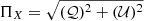 and ψX = 1/2 tan−1(𝒰/𝒬). Error estimation was calculated based on Kislat et al. (2015) and Muleri (2022). Figure 1 indicates the detection significance of this measurement in the form of a polarization contour plot.
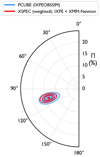 |
Fig. 1. Polarization contours from Obs. 4. Contours represent the significance of the time-averaged polarization detected with confidence levels of 68.27%, 90.00%, and 99.00%, with two degrees of freedom. The blue contour indicates the values of ΠX and ψX derived via the PCUBE methods, and the red contours show the same properties from simultaneous IXPE and XMM-Newton spectropolarimetric analysis. The radial and angular values represent ΠX and ψX, respectively, with the latter measured from north through east. |
The second method uses an event-based ML method to determine Q and (Marshall 2021b). The method accounts for background using data from an annulus about the target by including a term in the likelihood, as used in the analysis of the IXPE data of Cen A (Ehlert et al. 2022). Source events were selected from a region of 60″ radius about the source centroid, while the background events were selected from an annulus with inner and outer radii of 200″ and 300″. In this case, ΠX = 13 ± 1% and ψX = 107 ± 3°.
Next, the spectropolarimetric analysis examined the X-ray spectra and polarization properties based on spectral modeling with XSPEC (version 12.13.0c; Arnaud et al. 1996). With this method, we obtained ΠX = 14 ± 1% and ψX = 107 ± 3°. The detection significance of this measurement was ≳11σ. The flux was estimated as 2.25 (±0.04) × 10−10 erg s−1 cm−2 over 2–8 keV, the same band over which the IXPE I, Q, and U spectra were obtained. In this analysis, we additionally included the simultaneous XMM-Newton data in order to refine the constraints on the spectral shape over the 0.3–10 keV energy range. The cross-calibration factors among all the spectra are accounted for using the CONSTANT model, normalized to the XMM-Newton spectrum while the other spectra were varied. In all the fits, we considered the Galactic absorption along the line of sight of Mrk 421. For this, we used the TBABS model with weighted average column density values from HI4PI Collaboration (2016) (NH = 1.34 × 1020 cm−2). The WILM model was applied to take into account metal abundance (Wilms et al. 2000). For the spectral modeling, we first applied a simple power law model (POWERLAW in XSPEC) to reproduce the I synchrotron spectrum, but the best-fit result was poor, with χ2/d.o.f. = 3308/651. Hence, we employed the log-parabolic model (LOGPAR), in which the photon index varies with energy following a log parabola function Massaro et al. 2004:
 (1)
(1)
where the pivot energy Epivot is a scaling factor, α describes the slope of the photon spectrum at Epivot, β expresses the spectral curvature, and K denotes a normalization constant. This spectral model generally describes a typical HSP blazar spectrum well, including that of Mrk 421, both in quiescence and in flaring states (Donnarumma et al. 2009; Baloković et al. 2016). As the photon index varies with energy in this model, the choice of reference energy Epivot changes the determined value of α. In our spectral fit, we fixed the pivot energy to 5.0 keV (e.g., Baloković et al. 2016; Middei et al. 2022). In this case, the α parameter approximately corresponds to the photon index over 3.0–7.0 keV. In our spectral fitting, we also allowed the values of α, β, and K to vary. These free parameters are coupled with the reference spectrum, which here is the XMM-NewtonI spectrum over the same 2–8 keV band to which the three IXPE DUs are sensitive. Finally, the X-ray polarimetric measurements were constrained by the POLCONST model based on the Stokes parameter fits. Consequently, we obtained statistically acceptable fits, with χ2/d.o.f. = 740/650, above 99% confidence level. Figure A.1 and Table A.1 present the parameter values of our best-fit results. We note that in the Stokes-spectra-decoupled case, which only fits I spectra without involving POLCONST, the best-fit results obtained the same values as we derived from the simultaneous spectropolarimetric fit.
Finally, the MLS method was also applied to determine the polarization properties for the POWERLAW spectral model. With this procedure, we derived the polarization and spectral properties to be ΠX = 13 ± 1% and ψX = 109 ± 3°.
Therefore, the X-ray polarization properties we derived using four different methods are consistent within the uncertainties (see Table 1). The small differences can be explained by the fact that the PCUBE analysis estimated spectral-model-independent polarization properties, while the XSPEC methods take into account the best fit from the spectral modeling. Furthermore, among the current choices, only the XSPEC method can improve sensitivity by applying event weight methods introduced by Di Marco et al. (2022). Overall, we find that the ΠX and ψX results are robust, with modest statistical errors (see Fig. 1).
2.2. Polarization variability
We investigated whether the polarization varies as a function of time or energy. We tested the time dependence using two methods. In the first one, we determined the null-hypothesis probability with the χ2 test using the combined PCUBE and XSPEC analysis (e.g., Di Gesu et al. 2022, 2023; Gianolli et al. 2023). For the second method, we used the unbinned event-based ML analysis implemented in Marshall (2021a). With this method, we can avoid the error that can be caused by subjective selection bias resulting from the binning criteria.
The first method measured each normalized Stokes parameter value by dividing the data into identical time spans that depended on the selected number of bins (e.g., 2 bins = 100 ks/2 bins = 50 ks/bin). In particular, we split Obs. 4 into 2–20 time bins. We then compared 𝒬 and 𝒰, which followed a Gaussian error distribution, with the results from fitting each parameter treated as constant over time (i.e., 𝒬(t) = 𝒬0 and 𝒰(t) = 𝒰0). The result of fitting the constant model was calibrated for each number of bins. We then calculated the χ2 and the null-hypothesis probability (for the corresponding degrees of freedom) for each case. Figure 2 indicates the null-hypothesis probability as a function of the number of bins. In this figure, the green-shaded area (PNull > 1%) corresponds to cases where the data are statistically consistent with values of 𝒬 and 𝒰 that are constant in time. Conversely, if the points lie outside the region (PNull < 1%), it implies that the polarization varies with time. As seen in Fig. 2, we found that splitting the 𝒬(t) light curves with 5, 7, 8, 9, 11, 12, and 14 time bins does not produce a good fit with the constant model (PNull < 1%). The case of 7 time bins has the smallest null-hypothesis probability, with χ2/d.o.f. = 25.26/6, beyond the 3σ confidence level. In the polarization light curve of Obs. 4 with seven identical time bins (Fig. 3), we can see that ψX varies from the second to the fourth bin, after which it returns to a more stable value near that of the first three bins. We estimate the rotation rate of this variation as  °/day (change by 61° over ∼57 ks from the second to the fourth bin). This result is comparable to the rotation rate of
  reported in Di Gesu et al. (2023).
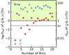 |
Fig. 2. Null-hypothesis probability of the χ2 test for time variability of the 𝒬 (red) and 𝒰 (blue) Stokes parameters with the constant model for different numbers of time bins for Obs. 4. The left and right vertical axes correspond to the probability values in logarithmic and linear scales, respectively. The green shaded area indicates that the null-hypothesis probability is above the 1% significance level. The dashed and dotted black lines located in the middle of the panel represent 1% and 3σ (99.73%) probability, respectively. |
Additionally, in order to examine the possibility of continuous change of ψX, we tested whether a sinusoidal function (ψX(t) = Asin(Ct − D)+B) provides a better fit of ψX(t) with respect to a constant function corresponding to the mean value of ψX over 7 time bins (blue line in Fig. 3). This approach yielded a smaller χ2/d.o.f. value of 4.75/3, with a Bayesian information criterion (BIC) of 12.53, than the constant model (χ2/d.o.f. = 16.66/6, BIC = 18.60).
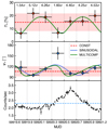 |
Fig. 3. IXPE polarization and photon counts versus time during Obs. 4. From top to bottom: ΠX, ψX, and count rates. Polarization results are from a time-resolved analysis with seven identical 19 ks time bins. The detection significance for each bin is displayed at the top of the figure. In the ΠX and ψX panels, dashed red lines denote a fit to a constant function; the shaded area corresponds to ≤3σ uncertainty. In addition, the solid blue and green lines indicate the best-fit result with the sinusoidal and multicomponent model, respectively. The dashed blue line in the light curve indicates the average value during the observation. |
As a second approach, we employed a ML method that allows for ψX rotation in each interval, as described elsewhere (Di Gesu et al. 2023) and shown in Fig. 4. Briefly, the ML method is used (see Sect. 2.1) for eight equal time intervals but also allowing for ψX rotation during the time interval, as an “uninteresting” parameter. This approach prevents ψX rotations during a time interval from reducing the average polarization of that interval, which is important when there are large ψX changes. For example, Fig. 4 shows that there appear to be large, nearly 90° ψX shifts between intervals one and two and between intervals three and four. As a result, we confirmed that ψX varied over time during Obs. 4 with ∼4.5σ confidence.
 |
Fig. 4. Time variability of the 𝒬 and 𝒰 Stokes parameters during Obs. 4. Each circle indicates the 1σ uncertainties of eight identical time intervals, derived using an event-based ML technique as described in Di Gesu et al. (2023). The black circle shows the time-averaged polarization. Each color represents a time interval from the start to the end of Obs. 4. |
In addition, with a ML method, we tested a more complex model fit – the multicomponent model (Pacciani et al., in prep.), which involves the convolution of constant and rotating polarization components – to check the possibility of continuous variation within the Obs. 4 period. The details of this model are described in Appendix B. From this test, we computed the significance of the multicomponent model relative to the constant polarization model based on the delta likelihood, ΔS′=S′(Π0, Ψ0, 0)−S′(Π1, Ψ1, Π2, Ψ2, ω). We obtained a decrease in the likelihood estimator, ΔL = −32.4, which follows a chi-square distribution with three degrees of freedom. Hence, the constant polarization model is rejected in favor of the multicomponent model, at the ∼5σ confidence level that this result occurred by chance. The parameters estimated with the multicomponent model are reported in Table 2. The observed discrepancy between the rotation rate measured from the multicomponent model (i.e., ω = 245 °/day) and the rate estimated directly from the light curve (i.e.,  ) can be explained by differences in physical interpretation. The multicomponent model assumes a persistent presence of the rotating component in conjunction with the constant emission component, while the other case assumes that the emission originates from a single dominant component. The multicomponent model is indicated with a green line in Fig. 3.
Parameters for the multicomponent model.
Therefore, based on these different methods, we conclude that we have found an episodic ψX variation over time during Obs. 4. Furthermore, the results of sinusoidal and multicomponent models suggest that the variations may be attributed to continuous changes in stable components. However, due to differences in the analysis methods employed, these two models were not compared in this study. Moreover, since these model fit results were derived as relative outcomes compared to the constant model, we cannot rule out the possibility of encountering more complex components and potential stochastic variations.
We also tested whether the X-ray polarization depends on energy by applying the same null-hypothesis probability test discussed above, but with the IXPE energy band (2–8 keV) divided into smaller ranges. We did so for two energy bins (2–4 and 4–8 keV), as well as three energy bins (2–4, 4–6, and 6–8 keV), up to 12 energy bins. We find no statistically significant differences with a constant fit, as PNull ≥ 13% from both 𝒬 and 𝒰; hence, the data are consistent with energy-independent X-ray polarization.
2.3. X-ray polarization and spectral variability across multiple IXPE observations
Significant X-ray polarization from Mrk 421 has been detected at four epochs with IXPE (see Table 1). Figure 5 shows error contours for both time-averaged and time-resolved data of each observation. Over the seven months from IXPE Obs. 1 to Obs. 4, the value of ψX varied widely, with a continuous rotation over 180° observed during Obs. 2 and Obs. 3. In contrast, measurements of ΠX for all events were similar within a range of 10-15%, even though the time-averaged ΠX of Obs. 2 and Obs. 3 appears to be clearly lower than in the other cases due to dilution by the changing of ψX. However, the mean value of ΠX during periods of non-rotation of ψX (Obs. 1 and Obs. 4) was 14 ± 2%, a factor of 1.4 ± 0.2 higher than the value of 10 ± 1% during the rotation (Obs. 2 and Obs. 3). This result is similar to the findings of previous optical polarimetry studies: (1) Blinov et al. (2016b) observed that the ratio of ΠO of rotating to that of nonrotating cases is less than 1 in 18 out of the 27 observed rotations, and (2) Jermak et al. (2016) reported a 26% reduction in the average ΠO during rotational periods compared to non-rotational periods. Nonetheless, because of the limited amount of X-ray polarization data, this result should be verified with an increased number of measurements from future X-ray polarimetry monitoring observations.
 |
Fig. 5. Time-averaged and time-resolved polarization contours of four multiple IXPE observations. In the top panel, each colored contour represents the significance of the time-averaged polarization detection for the corresponding observation (Obs. 1 in red, Obs. 2 in orange, Obs. 3 in green, and Obs. 4 in blue). Contours are shown at confidence levels of 68.27%, 90.00%, and 99.00%, as determined from a χ2 test with two degrees of freedom. Additionally, the black line and gray shaded areas indicate the jet’s electric-vector position angle in degrees as observed by the VLBA at 43 GHz (Obs. 1 is 100 ± 10°, Obs. 2 is 147 ± 7°, Obs. 3 is 147 ± 7°, and Obs. 4 is 171 ± 10°). In the bottom panel, the 99.00% confidence level contours show the time variation in polarization properties as determined by dividing the data into three identical time intervals for each observation. In the cases of Obs. 2 (orange) and Obs. 3 (green), arrows indicate a rotation of ψX from the start to the end of the observation. |
The radio electric-vector position angle ψ43 GHz obtained from the 43 GHz Very Long Baseline Array (VLBA) observations (black line in Fig. 5) differs from ψX and which also changes by 70° over the 7 months from Obs. 1 to Obs. 4. The pronounced variation in ψX and ψ43 GHz contrasts with the steadier X-ray polarization observed in other sources of the same subclass of blazars, whose synchrotron SED peaks at X-ray frequencies (i.e., Mrk 501; Liodakis et al. 2022).
We also investigated the spectral properties and X-ray activity of Mrk 421 through Swift-XRT monitoring observations. Figure 6 presents the α and β spectral parameters obtained from the LOGPAR model fit. We also derived the X-ray flux in the soft (0.3–2 keV), Fsoft, and hard (2–10 keV), Fhard, energy bands, and define the hardness ratio as (Fhard − Fsoft)/(Fhard + Fsoft). We have found that the α parameter, representing the slope of the spectrum at the pivot energy, maintained similar values in Obs. 1 and Obs. 4. However, during Obs. 2 and Obs. 3, α decreased with time. In addition, the hardness ratio also varied during the ψX rotation, while its value in Obs. 1 was consistent with that in Obs. 4. Nonetheless, in the case of Obs. 4, Swift-XRT observations were conducted only at the beginning and shortly after the IXPE pointing; thus, we cannot exclude the possibility of variations in spectral properties during Obs. 4.
 |
Fig. 6. Swift-XRT X-ray spectral parameters and flux versus time of Mrk 421 from a log-parabolic best-fit model with Epivot = 5 keV. From top to bottom: α, β, hardness ratio, and flux in the soft (0.3–2 keV, gray circles) and hard (2–10 keV, black diamonds) energy bands. The time ranges of the IXPE pointings are indicated by the gray shaded regions. |
The X-ray fluxes of Mrk 421 during all epochs of IXPE observations were within 1σ of the median historical value (e.g., Liodakis et al. 2019). Nonetheless, we found significant fluctuations during Obs. 2 and Obs. 3. Although the flux variations occurred during all of the IXPE epochs (see, e.g., Fig. 3), the discrepancy between the minimum and maximum counting rates was larger in Obs. 2 and Obs. 3. Therefore, we suggest that the smooth ψX rotation behavior may accompany more pronounced spectral and flux fluctuations.
3. Multiwavelength polarization analysis
Multiwavelength campaigns for the first three observations of Mrk 421 are reported in Di Gesu et al. (2022, 2023). During Obs. 4, Mrk 421 was observed with the VLBA, the Effelsberg 100-m Radio Telescope, the Korean VLBI Network (KVN), the Submillimeter Array (SMA), the Kanata Telescope, the Perkins Telescope, and the Sierra Nevada Observatory (SNO; T90 telescope). Details of the observations and observatories can be found in Appendix A.3.
We analyzed VLBA data obtained for Mrk 421 within the BEAM-ME (Blazars Entering the Astrophysical Multimessenger Era) program1 during the period from MJD 59616 (2022 February 5) to MJD 59986 (2023 February 11) to investigate the parsec-scale jet behavior during the IXPE observations. The data include total and polarized intensity images at 43 GHz at 12 epochs. The data reduction and modeling are described in Appendix A.4. The parsec-scale jet of Mrk 421 is strongly core-dominated, with the extended jet contributing an average of only 17% of the core flux density at 43 GHz. We consider the core to be a stationary feature of the jet and designate it as A0. During the one-year period analyzed here, we have detected two stationary features in the jet in addition to the core, A1 and A2, located at distances of ∼0.4 and ∼0.8 mas from A0, respectively (see Table A.3). Dominance by stationary structures is a well-documented property of the Mrk 421 jet (Lico et al. 2012; Jorstad et al. 2017; Lister et al. 2021; Weaver et al. 2022). Nonetheless, we have found motion in the jet, which we identify with a prominent polarized feature, P, which has a sub-luminal apparent speed βapp = 0.7 ± 0.1 in units of c. Figure 7 presents a sequence of images at epochs where the knot is prominent. Figure A.5 shows that knot P had a high degree of polarization, with ψP almost aligned with the jet direction, as expected if feature P was a transverse shock in the jet. According to its kinematics, the knot passed through the core on 2022 March 14 (MJD 59653 ± 80; Fig. A.3). If one considers the sizes of A0 and P listed in Table A.3, plus the proper motion of P (Appendix A.4), it should have taken 107 ± 19 days for knot P to leave the core completely, which should have occurred within 2022 June 10–July 8. This means that during IXPE Obs. 1, Obs. 2, and Obs. 3, knot P was within the millimeter-wave core.
 |
Fig. 7. VLBA total (contours) and polarized (color scale) intensity images of Mrk 421 at 43 GHz. The peak of the total intensity is 295 mJy beam−1. Yellow linear segments within the images indicate the direction of polarization, the black horizontal line marks the position of the core, A0, and colored circles indicate locations of jet features A1 (blue), A2 (gray), and P (red). Images are convolved with the same elliptical Gaussian beam, which is shown in the bottom-right corner by a black ellipse. |
The Effelsberg 100-m Telescope observation was obtained within the framework of the QUIVER program (Monitoring the Stokes Q, U, I and V Emission of AGN jets in Radio) on 2022 December 2 (MJD 59915.11). The linear polarization was measured at 3 bands: 4.85 GHz, 8.35 GHz and 10.45 GHz. Its polarization degree was found to be 0.9 ± 0.2%, 1.2 ± 0.4%, and 1.2 ± 0.2%. and its polarization angle 96.3 ± 3.5°, 134.8 ± 4.9°, and 159.2 ± 7.2°, respectively. The KVN observations, with the antennas combined to act as a single dish, were performed on 2022 December 9 (MJD 59922.73) at 22, 43, 86, and 129 GHz. The linear polarization was measured as Π22 GHz = 2.4 ± 0.7% along ψ22 GHz = 30 ± 12° at 22 GHz and Π43 GHz = 2.7 ± 0.5% along ψ43 GHz = 142 ± 9° at 43 GHz. The measured values of Π at 86 GHz (3.1 ± 2.3%) and 129 GHz (4.4 ± 2.0%) are not significant detections. The polarization was measured with the SMA at 225.5 GHz as Π225 GHz = 2.0 ± 0.3% along position angle ψ225 GHz = 163 ± 3°. At the same time, the intrinsic polarization degree (after subtraction of the host-galaxy flux) in the optical R band from SNO was ΠO = 4.6 ± 1.3% along ψO = 206 ± 9°. The Perkins telescope obtained optical R-band polarization covering Obs. 4 from 2022 November 26 (MJD 59909) to December 17 (MJD 59930) to give the average optical polarization parameters just before and after Obs. 4, which can be compared with the SNO measurement. In the infrared J and optical R bands, the Kanata Telescope data (not corrected for the host-galaxy depolarization) yield ΠJ = 2.41 ± 0.02% and ΠO = 2.1 ± 0.03% along ψJ = 176 ± 0.2° and ψO = 167.0 ± 0.3°, respectively. The latter is similar to previous Mrk 421 R-band observations with the Kanata Telescope, for which an intrinsic value of ΠO ≈ 3.3% was derived (Di Gesu et al. 2023), which is consistent with the SNO measurement. All of the new multiwavelength polarimetry results conducted during Obs. 4 are summarized in Table A.2.
Figure A.2 exhibits the evolution of polarization properties of Mrk 421 obtained from the contemporaneous multiwavelength polarimetry campaign from just before IXPE Obs. 1 to shortly after Obs. 4. Throughout this time period, we find a similar strong chromatic behavior, with 2–3 times higher Π at X-ray rather than at longer wavelengths. In contrast, the infrared, optical, and radio degrees of polarization were similar. Meanwhile, the polarization position angle exhibited marked changes, with different values during the various IXPE pointings. The range of ψ observed in Obs. 1 across millimeter to X-ray wavelengths was ∼30°, whereas a larger range of ∼90° was evident in Obs. 4. Moreover, Di Gesu et al. (2023) have reported that, during the rotation of ψX of Obs. 2 and Obs. 3, ψ values at other wavelengths were consistent with each other, with a weak temporal variation. Hence, we conclude that the region where the polarized X-rays are emitted is mostly or completely distinct from that at longer wavelengths.
Furthermore, Mrk 421 exhibited a clockwise ψO rotation of approximately 120° over ∼40 days during the first three IXPE observation periods. Similar behavior has been reported in previous optical polarimetry monitoring studies, where the polarization angle changed by ∼180° over ∼50 days (Blinov et al. 2015, 2016a, 2018; Jermak et al. 2016; Fraija et al. 2017). The direction of the ψO rotation was opposite to the counterclockwise ψX rotation observed by IXPE during Obs. 2 and Obs. 3.
4. Discussion
Previous IXPE observations of the HSP blazars Mrk 421 (Di Gesu et al. 2022, 2023) and Mrk 501 (Liodakis et al. 2022) suggest that an energy-stratified shock can most readily explain the ∼2–3 times higher degree of polarization at X-ray rather than at longer wavelengths. In this work, we have found consistent multiwavelength measurements from Obs. 4. In this energy-stratified shock model, the relativistic electrons convert their energy to radiation as they move farther from the shock front (Marscher & Gear 1985; Tavecchio et al. 2018). The particles are efficiently accelerated at the shock front, where the magnetic field is relatively well ordered, and hence emit X-ray synchrotron radiation with relatively high polarization. Conversely, electrons lose energy as they propagate away from the shock, causing them to radiate at longer wavelengths, and the degree of polarization decreases as they encounter increasingly turbulent magnetic fields (Di Gesu et al. 2022, 2023; Liodakis et al. 2022). Hence, higher Π is predicted at higher frequencies. This effect ceases at wavelengths long enough that the electrons radiating at those wavelengths can cross the entire shocked region before losing most of their energy (Marscher & Gear 1985). This limitation can explain the similar polarization from millimeter to optical wavelengths observed in Mrk 421. It is also possible that the longer wavelength emission occurred mainly in a relatively slow sheath surrounding a much faster X-ray emitting spine of the jet (e.g., Di Gesu et al. 2023). This is consistent with the sub-luminal speed we measured for knot P. In this case, the X-ray and longer wavelength polarization properties may not be related, consistent with their different position angles.
We therefore consider two possible geometries for an energy-stratified jet in Mrk 421: linear and radial models, as suggested by Di Gesu et al. (2022, 2023). In the case of linear geometry, the energy stratification and the ψ rotation can be explained by emission features propagating downstream in the jet, following the helical magnetic field. On the other hand, the radial structure can correspond to a helical, rotating innermost region and a surrounding layer, similar to the spine-sheath jet model (Chhotray et al. 2017). The currently available observational data are insufficient to discern between the linear and radial geometries. Nevertheless, the episodic variation in polarization observed during Obs. 4 offers further insights into the internal geometry of the jet. For instance, it implies alternative perspectives on the geometric structure within the jet, including the intricate interactions between coexisting stable and rotating magnetic field structures, as well as stochastic transitions within the dominant magnetic field structure responsible for particle acceleration. Therefore, future observations of polarization variability are expected to yield further evidence about the geometric structure inside the jet.
On the other hand, despite the comparable multiwavelength results reported for Mrk 421 and Mrk 501, we have found a difference in the behavior of ψX between them. In the case of Mrk 421, ψ43 GHz and ψX exhibited significant variations without any consistent alignment with either each other or the direction of the jet axis. However, in the case of Mrk 501, an alignment was observed (within the uncertainties) between measurements of the position angle of the jet axis, ψX, and ψ43 GHz conducted within a month of each other (Liodakis et al. 2022). Further IXPE and VLBA observations of HSP blazars are needed to confirm whether, and if so, why, Mrk 421 is different in this regard.
We have found that the X-ray flux and hardness ratio of Mrk 421 were less variable during Obs. 1 and Obs. 4, when ψX was essentially constant, than during the ψX rotation of Obs. 2 and Obs. 3. This implies different physical conditions within the jet between the rotating and nonrotating states. Instead, the similar values of ΠX across all observations suggest that the basic particle acceleration scenario remained roughly independent of the magnetic field geometry. This can be accommodated within the energy-stratified shock scenario, since the degree of order of the magnetic field could be similar whether the shock moves along a straight or helical trajectory. The flux and spectral variations during the rotation event could have been caused by changes in the Doppler factor as the shock executed helical motion, although the data are too sparsely sampled to test this. Future X-ray spectroscopic and polarimetric observations with improved time resolution can potentially test whether spiral motion along a helical magnetic field causes cyclical Doppler factor variations that lead to observed variations in flux, hardness ratio, and polarization. Our examination of a sequence of 43 GHz VLBA images has revealed the presence of a prominent, highly polarized knot moving away from the “core” at a speed of 0.7c during a time span that includes Obs. 1 – Obs. 3 (see Fig. A.3).
This finding suggests a potential connection between the morphological changes near the jet core region and the variability in polarization, as discussed in Di Gesu et al. (2023). The knot could represent a shock containing relativistic electrons accelerated up to Lorentz factor ∼106 that radiate at X-ray energies. However, in this scenario, it is difficult to explain the difference in the behavior of ψX between Obs. 1 and Obs. 2 – Obs. 3, unless the geometry of the magnetic field varies across the core, with a tighter helical structure toward the downstream end. However, our analysis does not indicate a direct connection between the X-ray polarization position angle and that of either the core or knot P (see Fig. A.5), although the degree of polarization of P, 15–20%, is comparable to ΠX. This apparent lack of connection supports the conclusion, drawn above, that emission regions at longer wavelengths (millimeter, infrared, and optical) were separate from, or only partially coincident with, that of the X-ray emission.
In the case of Obs. 4, there is no apparent connection between the values of ψ of the polarized features in the jet observed on 2022 December 6 (MJD 59919) and ψX (Fig. A.5). However, Fig. A.4 indicates an increase in the core flux density in 2023 February (MJD 59986) that could be a signature of an emerging moving feature that would have been upstream of the 43 GHz very-long-baseline interferometry (VLBI) core during IXPE Obs. 4. Further combined IXPE and VLBI monitoring could help in clarifying whether there is any relation between the X-ray emission regions and features seen in the jet at millimeter wavelengths.
We note that, from Obs. 1 to Obs. 3, the polarization angle at optical, infrared, and radio wavelengths rotated in the opposite direction relative to the 5-day rotation of ψX during Obs. 2 and Obs. 3. This finding supports the conclusion that the X-ray emission region is separate from that at longer wavelengths. The observed similarity in radio to optical polarization properties implies that the emission at these wavelengths originates from spatially interconnected regions. The longer (relative to X-ray) rotation timescale suggests that the X-ray emission region is smaller than that of these other wavelengths. Although the polarization vector rotation at longer wavelengths could be explained by propagation of a larger emission feature down a helical magnetic field (as in Fig. 8), the long-term behavior of the optical polarization of Mrk 421 implies stochastic, rather than systematic, variations in both ψO and ΠO (Marscher & Jorstad 2022).
 |
Fig. 8. Schematic diagram of double helical magnetic field components inside the jet. The downstream direction of the jet is to the left. The arrows indicate each helical magnetic field component involved in the emission at different wavelengths (X-ray in blue and longer wavelengths in black). |
5. Conclusions
We have reported X-ray, optical, infrared, and radio polarization and flux measurements of the HSP blazar Mrk 421, including four IXPE pointings from between 2022 May and December. Such observations probe the magnetic field structure and particle acceleration mechanisms inside the jets of blazars. The combined 7 months of observations sample the time and energy dependence of the X-ray polarization. Over this time span, ψX varied over the full range of ∼180°, including a 5-day episode of rotation, while the degree of polarization stayed between ∼10 and 15% across all IXPE pointings. The X-ray flux varied by a higher fraction during the rotation than during the two IXPE observations without rotations.
The simultaneous multiwavelength polarimetry results over four IXPE observations provide evidence useful for constraining the physics of the jet. The degree of X-ray polarization was typically ∼2–3 times greater than that at longer wavelengths at all epochs sampled, while the polarization angles fluctuated. The discrepancy between the X-ray results compared with radio, infrared, and optical polarimetry supports the previous conclusion that the X-ray emission region is distinct from that at longer wavelengths in HSP blazars (Liodakis et al. 2022; Di Gesu et al. 2022, 2023). As with previous studies, we conclude that the observations are consistent with the energy stratified shock model, with the level of turbulence increasing with distance from the shock front.
One difference between Mrk 421 and Mrk 501 is that there is no apparent correlation between the direction of the jet from VLBA and ψX in the former. While this could be due to the bending of the jet from the X-ray to the radio emitting region, amplified by the narrow angle to the line of sight, the optical polarization angle is also much more variable in Mrk 421 than in Mrk 501 (Marscher & Jorstad 2022). This implies an intrinsic difference between the two objects that should be explored with further observations.
Following Di Gesu et al. (2023), we propose a linear stratification scenario and a radial stratification scenario to explain the rotation behavior of ψX. The accompanying spectral variation during the ψX rotation suggests that the physical conditions of the jet, such as the energy distribution of relativistic electrons, differed between the periods of rotation and non-rotation. In addition, we report rotation in the opposite direction of the ψ between the X-ray and other wavelengths, with the latter occurring over a much longer timescale. This could potentially be interpreted as the presence of multi-helical magnetic field structures inside the jet. Morphological changes in the parsec-scale jet, possibly associated with the contemporaneous emergence of a new knot of emission observed to move down the jet in 43 GHz VLBA images, may be linked to the ψX rotation, although differences in the radio and X-ray polarization angles are evidence against such a connection.
In conclusion, the present study continues to develop a new perspective on the physical and geometrical features of the magnetic field inside the jets of blazars by employing polarimetry that extends from radio to X-ray wavelengths. The IXPE observations, which incorporate data at other wavelengths, have played a significant role in constraining the emission arising from the innermost regions of the jet. The polarization properties, sampled over different timescales and energy regimes, suggest a possible connection between spectral and polarization variations. The connection may include morphological changes in radio images, which coincided with a period of ψX rotation. However, due to infrequent data sampling, there remain uncertainties regarding apparent correlations, which can be chance coincidences. In addition, IXPE observations of Mrk 421 thus far have been obtained when the blazar was in average activity states. It is of great interest to determine whether the polarization and physical properties change during strong flaring events. As the IXPE mission continues, further studies of Mrk 421 and other blazars are expected to provide the data needed to improve our understanding of the magnetic field geometry and particle acceleration processes in relativistic jets.
http://www.bu.edu/blazars/BEAM-ME.html
The time of passage of the centroid of P through the centroid of A0
Acknowledgments
The authors thank the anonymous referee for comments that improved this manuscript. The Imaging X-ray Polarimetry Explorer (IXPE) is a joint US and Italian mission. The US contribution is supported by the National Aeronautics and Space Administration (NASA) and led and managed by its Marshall Space Flight Center (MSFC), with industry partner Ball Aerospace (contract NNM15AA18C). The Italian contribution is supported by the Italian Space Agency (Agenzia Spaziale Italiana, ASI) through contract ASI-OHBI-2017-12-I.0, agreements ASI-INAF-2017-12-H0 and ASI-INFN-2017.13-H0, and its Space Science Data Center (SSDC), and by the Istituto Nazionale di Astrofisica (INAF) and the Istituto Nazionale di Fisica Nucleare (INFN) in Italy. This research used data products provided by the IXPE Team (MSFC, SSDC, INAF, and INFN) and distributed with additional software tools by the High-Energy Astrophysics Science Archive Research Center (HEASARC), at NASA Goddard Space Flight Center (GSFC). The IAA-CSIC group acknowledges financial support from the grant CEX2021-001131-S funded by MCIN/AEI/10.13039/501100011033 to the Instituto de Astrofísica de Andalucía-CSIC and through grant PID2019-107847RB-C44. The QUIVER data are based on observations with the 100-m Telescope of the MPIfR (Max-Planck-Institut für Radioastronomie) at Effelsberg. Observations with the 100-m radio Telescope at Effelsberg have received funding from the European Union’s Horizon 2020 research and innovation programme under grant agreement No 101004719 (ORP). The POLAMI observations were carried out at the IRAM 30m Telescope. IRAM is supported by INSU/CNRS (France), MPG (Germany), and IGN (Spain). Some of the data are based on observations collected at the Observatorio de Sierra Nevada, owned and operated by the Instituto de Astrofísica de Andalucía (IAA-CSIC). Further data are based on observations collected at the Centro Astronómico Hispano en Andalucía (CAHA), operated jointly by Junta de Andalucía and Consejo Superior de Investigaciones Científicas (IAA-CSIC). The Submillimetre Array is a joint project between the Smithsonian Astrophysical Observatory and the Academia Sinica Institute of Astronomy and Astrophysics and is funded by the Smithsonian Institution and the Academia Sinica. Mauna Kea, the location of the SMA, is a culturally important site for the indigenous Hawaiian people; we are privileged to study the cosmos from its summit. Some of the data reported here are based on observations made with the Nordic Optical Telescope, owned in collaboration with the University of Turku and Aarhus University, and operated jointly by Aarhus University, the University of Turku, and the University of Oslo, representing Denmark, Finland, and Norway, the University of Iceland and Stockholm University at the Observatorio del Roque de los Muchachos, La Palma, Spain, of the Instituto de Astrofisica de Canarias. E. L. was supported by Academy of Finland projects 317636 and 320045. The data presented here were obtained [in part] with ALFOSC, which is provided by the Instituto de Astrofisica de Andalucia (IAA) under a joint agreement with the University of Copenhagen and NOT. We acknowledge funding to support our NOT observations from the Finnish Centre for Astronomy with ESO (FINCA), University of Turku, Finland (Academy of Finland grant nr 306531). We are grateful to Vittorio Braga, Matteo Monelli, and Manuel Sänchez Benavente for performing the observations at the Nordic Optical Telescope. Part of the French contributions is supported by the Scientific Research National Center (CNRS) and the French spatial agency (CNES). The research at Boston University was supported in part by National Science Foundation grant AST-2108622, NASA Fermi Guest Investigator grants 80NSSC21K1917 and 80NSSC22K1571, and NASA Swift Guest Investigator grant 80NSSC22K0537. This study was based in part on observations conducted using the Perkins Telescope Observatory (PTO) in Arizona, USA, which is owned and operated by Boston University. This research was conducted in part using the Mimir instrument, jointly developed at Boston University and Lowell Observatory and supported by NASA, NSF, and the W.M. Keck Foundation. We thank D. Clemens for guidance in the analysis of the Mimir data. This work was supported by JST, the establishment of university fellowships toward the creation of science and technology innovation, Grant Number JPMJFS2129. This work was supported by Japan Society for the Promotion of Science (JSPS) KAKENHI Grant Numbers JP21H01137. This work was also partially supported by the Optical and Near-Infrared Astronomy Inter-University Cooperation Program from the Ministry of Education, Culture, Sports, Science and Technology (MEXT) of Japan. We are grateful to the observation and operating members of the Kanata Telescope. This research has made use of data from the RoboPol program, a collaboration between Caltech, the University of Crete, IA-FORTH, IUCAA, the MPIfR, and the Nicolaus Copernicus University, which was conducted at Skinakas Observatory in Crete, Greece. D.B., S.K., R.S., N. M., acknowledge support from the European Research Council (ERC) under the European Unions Horizon 2020 research and innovation program under grant agreement No. 771282. C.C. acknowledges support from the European Research Council (ERC) under the HORIZON ERC Grants 2021 program under grant agreement No. 101040021. We acknowledge the use of public data from the Swift data archive. Based on observations obtained with XMM-Newton, an ESA science mission with instruments and contributions directly funded by ESA Member States and NASA. The Very Long Baseline Array is an instrument of the National Radio Astronomy Observatory. The National Radio Astronomy Observatory is a facility of the National Science Foundation operated under a cooperative agreement by Associated Universities, Inc. S. Kang, S.-S. Lee, W. Y. Cheong, S.-H. Kim, and H.-W. Jeong were supported by the National Research Foundation of Korea (NRF) grant funded by the Korea government (MIST) (2020R1A2C2009003). The KVN is a facility operated by the Korea Astronomy and Space Science Institute. The KVN operations are supported by KREONET (Korea Research Environment Open NETwork) which is managed and operated by KISTI (Korea Institute of Science and Technology Information). The VLBA is an instrument of the National Radio Astronomy Observatory. The National Radio Astronomy Observatory is a facility of the National Science Foundation operated under cooperative agreement by Associated Universities, Inc.
References
- Abdo, A. A., Ackermann, M., Agudo, I., et al. 2010, ApJ, 716, 30 [NASA ADS] [CrossRef] [Google Scholar]
- Agudo, I., Thum, C., Wiesemeyer, H., et al. 2012, A&A, 541, A111 [NASA ADS] [CrossRef] [EDP Sciences] [Google Scholar]
- Aharonian, F. A. 2000, New Astron., 5, 377 [NASA ADS] [CrossRef] [Google Scholar]
- Akitaya, H., Moritani, Y., Ui, T., et al. 2014, in Ground-based and Airborne Instrumentation for Astronomy V, eds. S. K. Ramsay, I. S. McLean, & H. Takami, SPIE Conf. Ser., 9147, 91474O [NASA ADS] [Google Scholar]
- Arnaud, K. A. 1996, in Astronomical Data Analysis Software and Systems V, eds. G. H. Jacoby, & J. Barnes, ASP Conf. Ser., 101, 17 [NASA ADS] [Google Scholar]
- Aumont, J., Conversi, L., Thum, C., et al. 2010, A&A, 514, A70 [NASA ADS] [CrossRef] [EDP Sciences] [Google Scholar]
- Baldini, L., Barbanera, M., Bellazzini, R., et al. 2021, Astropart. Phys., 133, 102628 [NASA ADS] [CrossRef] [Google Scholar]
- Baldini, L., Bucciantini, N., Lalla, N. D., et al. 2022, SoftwareX, 19, 101194 [NASA ADS] [CrossRef] [Google Scholar]
- Baloković, M., Paneque, D., Madejski, G., et al. 2016, ApJ, 819, 156 [Google Scholar]
- Bellazzini, R., Angelini, F., Baldini, L., et al. 2003, in Polarimetry in Astronomy, ed. S. Fineschi, SPIE Conf. Ser., 4843, 372 [NASA ADS] [CrossRef] [Google Scholar]
- Bellazzini, R., Spandre, G., Minuti, M., et al. 2007, Nucl. Instrum. Methods Phys. Res. A, 579, 853 [CrossRef] [Google Scholar]
- Blinov, D., Pavlidou, V., Papadakis, I., et al. 2015, MNRAS, 453, 1669 [NASA ADS] [CrossRef] [Google Scholar]
- Blinov, D., Pavlidou, V., Papadakis, I. E., et al. 2016a, MNRAS, 457, 2252 [NASA ADS] [CrossRef] [Google Scholar]
- Blinov, D., Pavlidou, V., Papadakis, I., et al. 2016b, MNRAS, 462, 1775 [NASA ADS] [CrossRef] [Google Scholar]
- Blinov, D., Pavlidou, V., Papadakis, I., et al. 2018, MNRAS, 474, 1296 [CrossRef] [Google Scholar]
- Böttcher, M. 2019, Galaxies, 7, 20 [Google Scholar]
- Böttcher, M., Reimer, A., Sweeney, K., & Prakash, A. 2013, ApJ, 768, 54 [Google Scholar]
- Chhotray, A., Nappo, F., Ghisellini, G., et al. 2017, MNRAS, 466, 3544 [NASA ADS] [CrossRef] [Google Scholar]
- Costa, E., Soffitta, P., Bellazzini, R., et al. 2001, Nature, 411, 662 [NASA ADS] [CrossRef] [Google Scholar]
- Dermer, C. D., & Schlickeiser, R. 1993, ApJ, 416, 458 [Google Scholar]
- Di Gesu, L., Donnarumma, I., Tavecchio, F., et al. 2022, ApJ, 938, L7 [CrossRef] [Google Scholar]
- Di Gesu, L., Marshall, H. L., Ehlert, S. R., et al. 2023, Nat. Astron., 7, 1245 [NASA ADS] [CrossRef] [Google Scholar]
- Di Marco, A., Costa, E., Muleri, F., et al. 2022, AJ, 163, 170 [NASA ADS] [CrossRef] [Google Scholar]
- Di Marco, A., Soffitta, P., Costa, E., et al. 2023, AJ, 165, 143 [CrossRef] [Google Scholar]
- Donnarumma, I., Vittorini, V., Vercellone, S., et al. 2009, ApJ, 691, L13 [NASA ADS] [CrossRef] [Google Scholar]
- Ehlert, S. R., Ferrazzoli, R., Marinucci, A., et al. 2022, ApJ, 935, 116 [NASA ADS] [CrossRef] [Google Scholar]
- Fabiani, S., Costa, E., Bellazzini, R., et al. 2012, Adv. Space Res., 49, 143 [NASA ADS] [CrossRef] [Google Scholar]
- Fabiani, S., & Muleri, F. 2014, Astronomical X-Ray Polarimetry, Astronomia e astrofisica (Aracne) [Google Scholar]
- Fossati, G., Maraschi, L., Celotti, A., Comastri, A., & Ghisellini, G. 1998, MNRAS, 299, 433 [Google Scholar]
- Fraija, N., Benítez, E., Hiriart, D., et al. 2017, ApJS, 232, 7 [Google Scholar]
- Gianolli, V. E., Kim, D. E., Bianchi, S., et al. 2023, MNRAS, 523, 4468 [NASA ADS] [CrossRef] [Google Scholar]
- HI4PI Collaboration (Ben Bekhti, N., et al.) 2016, A&A, 594, A116 [NASA ADS] [CrossRef] [EDP Sciences] [Google Scholar]
- Ho, P. T. P., Moran, J. M., & Lo, K. Y. 2004, ApJ, 616, L1 [Google Scholar]
- Hovatta, T., & Lindfors, E. 2019, New Astron. Rev., 87, 101541 [CrossRef] [Google Scholar]
- Hovatta, T., Lindfors, E., Blinov, D., et al. 2016, A&A, 596, A78 [NASA ADS] [CrossRef] [EDP Sciences] [Google Scholar]
- Jermak, H., Steele, I. A., Lindfors, E., et al. 2016, MNRAS, 462, 4267 [NASA ADS] [CrossRef] [Google Scholar]
- Jones, T. W., O’Dell, S. L., & Stein, W. A. 1974, ApJ, 188, 353 [NASA ADS] [CrossRef] [Google Scholar]
- Jorstad, S. G., Marscher, A. P., Morozova, D. A., et al. 2017, ApJ, 846, 98 [Google Scholar]
- Kang, S., Lee, S.-S., & Byun, D.-Y. 2015, J. Korean Astron. Soc., 48, 257 [NASA ADS] [CrossRef] [Google Scholar]
- Kawabata, K. S., Okazaki, A., Akitaya, H., et al. 1999, PASP, 111, 898 [NASA ADS] [CrossRef] [Google Scholar]
- Kislat, F., Clark, B., Beilicke, M., & Krawczynski, H. 2015, Astropart. Phys., 68, 45 [NASA ADS] [CrossRef] [Google Scholar]
- Kraus, A., Krichbaum, T. P., Wegner, R., et al. 2003, A&A, 401, 161 [NASA ADS] [CrossRef] [EDP Sciences] [Google Scholar]
- Lico, R., Giroletti, M., Orienti, M., et al. 2012, A&A, 545, id A117 [NASA ADS] [CrossRef] [EDP Sciences] [Google Scholar]
- Liodakis, I., Peirson, A. L., & Romani, R. W. 2019, ApJ, 880, 29 [NASA ADS] [CrossRef] [Google Scholar]
- Liodakis, I., Marscher, A. P., Agudo, I., et al. 2022, Nature, 611, 677 [CrossRef] [Google Scholar]
- Lister, M. L., Homan, D. C., Kellermann, K. I., et al. 2021, ApJ, 923, 30 [NASA ADS] [CrossRef] [Google Scholar]
- Mannheim, K. 1993, A&A, 269, 67 [NASA ADS] [Google Scholar]
- Maraschi, L., Ghisellini, G., & Celotti, A. 1992, ApJ, 397, L5 [CrossRef] [Google Scholar]
- Marrone, D. P., & Rao, R. 2008, in Millimeter and Submillimeter Detectors and Instrumentation for Astronomy IV, eds. W. D. Duncan, W. S. Holland, S. Withington, & J. Zmuidzinas, SPIE Conf. Ser., 7020, 70202B [NASA ADS] [CrossRef] [Google Scholar]
- Marscher, A. P., & Gear, W. K. 1985, ApJ, 298, 114 [Google Scholar]
- Marscher, A. P., & Jorstad, S. G. 2022, Universe, 8, 644 [NASA ADS] [CrossRef] [Google Scholar]
- Marscher, A. P., Jorstad, S. G., D’Arcangelo, F. D., et al. 2008, Nature, 452, 966 [Google Scholar]
- Marscher, A. P., Jorstad, S. G., Larionov, V. M., et al. 2010, ApJ, 710, L126 [Google Scholar]
- Marshall, H. L. 2021a, ApJ, 907, 82 [NASA ADS] [CrossRef] [Google Scholar]
- Marshall, H. L. 2021b, AJ, 162, 134 [NASA ADS] [CrossRef] [Google Scholar]
- Massaro, E., Perri, M., Giommi, P., & Nesci, R. 2004, A&A, 413, 489 [NASA ADS] [CrossRef] [EDP Sciences] [Google Scholar]
- Middei, R., Giommi, P., Perri, M., et al. 2022, MNRAS, 514, 3179 [NASA ADS] [CrossRef] [Google Scholar]
- Middei, R., Perri, M., Puccetti, S., et al. 2023, ApJ, 953, L28 [NASA ADS] [CrossRef] [Google Scholar]
- Muleri, F. 2022, in Handbook of X-ray and Gamma-ray Astrophysics, eds. C. Bambi, & A. Santangelo (Springer Living Reference Work), 6 [Google Scholar]
- Myserlis, I., Angelakis, E., Kraus, A., et al. 2018, A&A, 609, A68 [NASA ADS] [CrossRef] [EDP Sciences] [Google Scholar]
- Nilsson, K., Pasanen, M., Takalo, L. O., et al. 2007, A&A, 475, 199 [NASA ADS] [CrossRef] [EDP Sciences] [Google Scholar]
- Piconcelli, E., Jimenez-Bailón, E., Guainazzi, M., et al. 2004, MNRAS, 351, 161 [Google Scholar]
- Primiani, R. A., Young, K. H., Young, A., et al. 2016, J. Astron. Instrum., 5, 1641006 [NASA ADS] [CrossRef] [Google Scholar]
- Rankin, J., Muleri, F., Tennant, A. F., et al. 2022, AJ, 163, 39 [NASA ADS] [CrossRef] [Google Scholar]
- Rybicki, G. B., & Lightman, A. P. 1979, Radiative Processes in Astrophysics (New York: Wiley) [Google Scholar]
- Sikora, M., Begelman, M. C., & Rees, M. J. 1994, ApJ, 421, 153 [Google Scholar]
- Strohmayer, T. E. 2017, ApJ, 838, 72 [NASA ADS] [CrossRef] [Google Scholar]
- Tavecchio, F. 2021, Galaxies, 9, 37 [NASA ADS] [CrossRef] [Google Scholar]
- Tavecchio, F., Landoni, M., Sironi, L., & Coppi, P. 2018, MNRAS, 480, 2872 [NASA ADS] [CrossRef] [Google Scholar]
- Weaver, Z. R., Jorstad, S. G., Marscher, A. P., et al. 2022, ApJS, 260, 12 [NASA ADS] [CrossRef] [Google Scholar]
- Weisskopf, M. C., Soffitta, P., Baldini, L., et al. 2022, J. Astron. Telesc. Instrum. Syst., 8, 026002 [NASA ADS] [CrossRef] [Google Scholar]
- Wilms, J., Allen, A., & McCray, R. 2000, ApJ, 542, 914 [Google Scholar]
- Zhang, H. 2019, Galaxies, 7, 85 [NASA ADS] [CrossRef] [Google Scholar]
Appendix A: Observation and data reduction
A.1. IXPE data
We obtained cleaned level 2 IXPE data processed by a standard IXPE pipeline from the Science Operation Center (SOC)2. The pipeline includes the photoelectron events correction in the GPD (Costa et al. 2001; Bellazzini et al. 2007; Fabiani et al. 2012; Baldini et al. 2021), as well as the photo-electron track reconstruction process based on standard moments analysis (Bellazzini et al. 2003; Fabiani & Muleri 2014; Di Marco et al. 2022). In particular, the pipeline rectifies the fluctuations in gain properties affected by gas conditions (e.g., temperature and pressure), nonuniform charging of the gas electron multiplier material, and polarization artifacts induced by spurious modulation (Rankin et al. 2022). The level 2 data of IXPE contain the time of arrival, position, and energy of each photon event, along with polarization information represented by the Q and Stokes parameters.
The scientific data analysis was performed using the public ixpeobssim software version 30.2.1 (Baldini et al. 2022). First, we extracted the source and background data using an optimized region selection criterion as suggested by Di Marco et al. (2023). The source data were extracted from a circular region with a 60″radius, while the background data were extracted from an annular source-free region with inner and outer radii of 150″and 300″, respectively. Both regions were centered on the source position in the detector frame. Next, we created the polarization cube (PCUBE) and the Stokes parameter spectra (I, Q, and ) using xpbin. To eliminate the influence due to the background, we applied the background subtraction technique (Baldini et al. 2022) and created PCUBEs of the source and background for each DU. The final source polarization properties were recalibrated by considering the BACKSCALE ratio between the source and background (∼0.05). In a similar way, we produced three Stokes parameter spectra for three detectors, totaling 9 spectra, using the PHA1, PHAQ, and PHAU algorithms in xpbin. We grouped the Ispectra with a minimum of 30 counts in each energy bin, as required for the χ2 statistics in the fits, and applied constant energy binning for the Qand spectra for every 0.2 keV interval. We employed the recent version of the IXPE calibration database files (CALDB 20221020) contained in both ixpeobssim and the HEASOFT package (v6.31.1) for both the PCUBE and the Stokes parameter spectra. In particular, we utilized the weighted analysis method (Di Marco et al. 2022) on the I, Q, and spectra to improve the significance of our measurements with alpha075 response matrices. The flux variability was analyzed using a light curve created with the LC algorithms in xpbin of ixpeobssim.
The polarization error contour (Fig. 1) was drawn from calibrated normalized 𝒬 (=Q/I) and 𝒰 (=U/I) at specific confidence levels (68.27%, 90.00%, and 99.00%) according to
 (A.1)
(A.1)
where 𝒬0 and 𝒰0 represent the averaged Stokes parameter values, and 𝒬C.L. and 𝒰C.L. denote the 𝒬 and 𝒰 values of a given confidence level calculated with two degrees of freedom, respectively. We note that, since we are considering two dependent variables, Π and ψ, at the same time, the error should be recalculated based on the χ2 distribution with 2 degrees of freedom (ϵ = σ
 , σ = σ𝒬 = σ𝒰). The variable ζ follows the angle distribution from 0 to 2π.
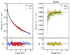 |
Fig. A.1. Spectropolarimetric fit of XMM-Newton (blue) and IXPE I (red), Q (green), and (orange) spectra, with residuals of the best-fit model. The left panel displays the I spectrum with a log-parabolic model (Massaro et al. 2004), while the right panel presents the constant polarization model fit with the POLCONST model for Q and spectra. The black line in both panels indicates the model fit result. |
Best-fit parameters from our simultaneous spectropolarimetric analysis.
A.2. Spectroscopic X-ray data
During IXPE Obs. 4, a snapshot of about 5 ks was performed with XMM-Newton in timing mode to limit photon pile-up. To extract the science products, we used the XMM-Newton Science Analysis Software (SAS), version 21, with the most updated current calibration files. Two boxed regions were adopted to extract the source spectra and background. In particular, we chose the source box to have a width of 27 pixels, as this size was found to maximize the signal-to-noise ratio. (Details of this procedure can be found in Piconcelli et al. 2004.) Then, the resulting spectrum was binned to achieve at least 30 counts in each energy bin. To allow simultaneous spectropolarimetric fitting within XSPEC, the keyword “XFLT0001 Stokes:0” was added to the headers of the corresponding PHA files.
The Swift-XRT monitoring consisted of ∼1 ks long observations performed in windowed timing (WT) mode. Raw data were reduced using the standard commands within the XRT Data Analysis Software (XRTDAS, version 3.6.1) and adopting the latest calibration files available in the Swift-XRT CALDB (version 20210915). The cleaned event files were used to extract the source spectrum from a circular region with a radius of 47″, while the background was extracted using a blank sky WT observation available in the Swift archive, also within a circular region of radius 47″. The resulting spectra were subsequently binned, requiring at least 25 counts in each energy bin.
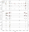 |
Fig. A.2. Multiwavelength polarization versus time of Mrk 421. Each row presents the polarization degree (circle) and polarization angle (triangle), with 1σ errors measured by radio (f < 50 GHz in red, 50 < f < 100 GHz in yellow, 100 < f < 200 GHz in green, and f < 200 GHz in blue), infrared (green), optical (red), and X-ray (orange) facilities, from top to bottom. The gray shaded areas denote the durations of the four IXPE observations. |
Multiwavelength polarization properties of Mrk 421.
A.3. Radio, infrared, and optical data
During all of the IXPE pointings, we observed Mrk 421 at millimeter (radio), infrared, and optical wavelengths, measuring both flux density and linear polarization. The observations and data analysis for the first three observations can be found in detail in Di Gesu et al. (2022, 2023); here we provide only a short description. For Obs. 4, radio, infrared, and optical observations were provided by QUIVER at the Effelsberg telescope, KVN, SMA (Ho et al. 2004), Hiroshima Optical and Near-InfraRed camera (HONIR; Akitaya et al. 2014) at the Kanata Telescope, the Perkins Telescope, and T90 at the SNO.
The QUIVER observations were performed at several radio bands (depending on receiver availability and weather conditions) from 2.6 GHz to 44 GHz (11 cm to 7 mm wavelength) using six receivers located at the secondary focus of the 100-m Effelsberg Radio Telescope (S110mm, S45mm, S28mm, S20mm, S14mm, and S7mm). The receivers are equipped with two orthogonally polarized feeds (either circular or linear) that can deliver polarimetric parameters either using conventional polarimeters or by connecting the SpecPol spectropolarimetric backend. Instrumental polarization is calibrated via observations of both polarized and unpolarized calibrators performed in each session, and then removed from the data (e.g., Myserlis et al. 2018; Kraus et al. 2003). The polarized intensity, degree, and position angle were derived from the Stokes I, Q, and cross-scans. The total flux density was successfully recovered at 13 bands between 4.85 GHz and 43.75 GHz. The calibrators 3C 286, 3C 48, and NGC 7027 were used for the total flux and polarization calibration (e.g., Myserlis et al. 2018; Kraus et al. 2003).
Observations were conducted with the KVN simultaneously at 4 frequencies from 22 to 129 GHz in single-dish mode. This was achieved by using the Tamna (22, 43 GHz) and Yonsei (86,129 GHz) antennas with circularly polarized feed horns to conduct two-frequency dual-polarization observations. The polarization angle was calibrated using the Crab nebula (152°; Aumont et al. 2010), and the polarization degree using Jupiter (unpolarized) and 3C286 (polarized, Agudo et al. 2012) following Kang et al. (2015).
The SMA observations were taken at 225.538 GHz (1.3 mm) through the SMAPOL (SMA Monitoring of AGN with POLarization) program. The SMAPOL observations were taken on 2022 December 7 (MJD 59920) in full polarization mode (Marrone & Rao 2008) using the SWARM correlator (Primiani et al. 2016), and calibrated with the MIR software package3.
Observations using HONIR were taken on 2022 December 6 (MJD 59919.7537) in the R and J bands4. Each observation comprised four exposures in different positions of the half-wave plate (Kawabata et al. 1999), which were then used to estimate the Stokes parameters and calculate the polarization degree and angle. The host galaxy of Mrk 421 contributes a significant fraction of unpolarized flux to the total emission, thereby reducing the polarization. None of the polarization degree estimates from Kanata have been corrected for the host-galaxy contribution due to the lack of the photometry data needed for such a correction, and hence they should be considered as lower limits to the intrinsic polarization degree of the blazar component.
The optical photometric and polarimetric observations were also obtained at the 1.8 m Perkins Telescope (Flagstaff, AZ, USA) with the PRISM camera5 in the R band performed before and after Obs. 4. The camera includes a polarimeter with a rotating half-wave plate. Each polarization observation has consisted of four consecutive exposures of 60 s at instrumental position angles 0°, 90°, 45°, and 135° of the wave plate to calculate the normalized Stokes parameters Q and U.
The SNO observations were performed using polarized filters oriented to represent different positions of a half-wave plate, similar to a conventional polarimeter. The data are then analyzed following standard photometric procedures. Mrk 421 was observed on 2022 December 7 in the R band. In this case, following Nilsson et al. (2007) and Hovatta et al. (2016), we corrected the host-galaxy contribution. Several observations were taken within the same night. We report the weighted average and uncertainty after considering all of the intra-night observations to account for variations in the system and the observing conditions during the rotation of the filter wheel.
A.4. VLBA observations and analysis
The VLBA data were reduced with the Astronomical Image Process System (AIPS) and Difmap software packages in the manner described by Jorstad et al. (2017). The total intensity images are modeled by a number of components with circular Gaussian brightness distributions, with the minimum number of components determined by the best fit between the data and model at each epoch according to a χ2 test. We identify the brightest feature located at the southeastern end of the jet as the “core,” designated as A0, which we assume to be a stationary feature. To obtain polarized intensity images, the data were corrected for the instrumental-polarization “D-terms,” calculated by averaging the D-terms obtained individually from a number of sources (usually 15) observed along with Mrk 421 in the BEAM-ME program. The electric-vector position angle (ψ43GHz) calibration was obtained by different methods, as discussed in Jorstad et al. (2017). The modeling of total intensity images provides the following parameters of each component: flux density, S, distance from the core, R, position angle with respect to the core, Θ, and angular size of the component, a (full width at half maximum of the best-fit Gaussian). For polarized features in the jet, we calculated the degree of polarization, Πknot, and ψknot by integrating the Q and U Stokes parameter models obtained with Difmap during imaging within the size of the corresponding feature from the total flux density modeling. As a result of modeling, we have detected three stationary features, A0, A1, and A2, and one moving knot, P in the jet of Mrk 421 during 12 epochs from 2022 February 5 to 2023 February 11. Table A.3 gives the average (over epochs) parameters of the jet features, while Fig. A.3 plots the distance of all knots detected in the jet versus time, and Fig. A.4 presents the light curve of the core, A0.
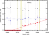 |
Fig. A.3. Distance from the core of jet components A1 (blue circles), A2 (gray circles), and P (red circles) versus time. The black dotted line indicates the position of the core, A0, the red line approximates the motion of knot P with the uncertainty of its ejection time shown by the red area at the bottom left, and yellow areas mark epochs of IXPE observations. |
Average parameters of the main features in the jet of Mrk 421 at 43 GHz.
We approximated the motion of knot P with a ballistic trajectory with proper motion μ = 0.34±0.06 mas yr−1, corresponding to a sub-luminal apparent speed (in units of c) βapp = 0.7 ± 0.1. The MOJAVE survey 6 at 15 GHz finds an historical maximum βapp ∼ 0.2 in the Mrk 421 jet. At 43 GHz, with 3 times higher angular resolution, Weaver et al. (2022) reported three knots with βapp > 1, with the fastest having an apparent speed of 2.41 ± 0.14 c, based on monitoring within the VLBA-BU-BLAZAR program. We extrapolated the motion of P back to the core (as shown in Fig. A.3 by a solid red line), which yields the time of ejection of P from the core 7 as MJD 59653±80 (2022 March 14). Figure A.4 plots the light curve of the core (A0), which has a local maximum on MJD 59699 (2022 April 30), the epoch of VLBA observation closest to the ejection time of P; this supports the derived time of ejection. Knot P possesses the highest degree of polarization in the jet, with ΠP reaching ∼20%. Another polarized feature in the jet is the core A0, with an average ΠA0 ∼ 2%. Figure A.5 shows the evolution of the polarization parameters ΠA0, ψA0 and ΠP, ψP. Figures A.3 and A.5 also indicate the times of the four IXPE observations by yellow areas, with the widest area covering two pointings (Obs. 2 and Obs. 3). Figure A.5 plots the values of ΠX and ψX, except during observations Obs. 2 & Obs. 3, when ψX rotated at a fast rate of ∼85 °/day (Di Gesu et al. 2023).
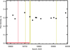 |
Fig. A.4. Light curve of the core, A0. The red vertical line marks the time of the ejection of knot P, with its 1σ uncertainty indicated by the red horizontal line. The yellow areas mark epochs of IXPE observations. |
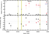 |
Fig. A.5. Polarization parameters of component A0 (black circles) and P (red circles): the degree of polarization (top panel) and the position angle of polarization (bottom panel). The yellow areas mark IXPE observations, while blue triangles plot ΠX and ψX; the dashed gray line in the bottom panel shows the direction of the jet according to Weaver et al. (2022), with dotted gray lines indicating its 1σ uncertainty. |
Appendix B: Maximum likelihood method of the multicomponent model
The multicomponent model (Pacciani et al., in preparation) comprises (1) a constant component with a steady polarization degree and angle and (2) a rotating component with a constant polarization degree and a rotating polarization angle. The likelihood estimator for this model is
![Mathematical equation: $$ \begin{aligned}&S(\Pi _1,\Psi _1,\Pi _2,\Psi ^0_2,R_1,\omega )=\nonumber \\&-2\sum _i \ln \biggr [ 1+\mu _iR_1\Pi _1\left(\cos 2\Psi _1\cos 2\psi _i+\sin 2\Psi _1\sin 2\psi _i\right)+ \nonumber \\&\mu _i(1-R_1)\Pi _2\left(\cos 2\Psi ^0_2\cos 2(\psi _i-\omega t)+\sin 2\Psi ^0_2\sin 2(\psi _i-\omega t) \right)\biggr ], \end{aligned} $$](/articles/aa/full_html/2024/01/aa47408-23/aa47408-23-eq9.gif) (B.1)
(B.1)
where Π1 and Ψ1 are the polarization degree and angle of the constant component; Π2 is the polarization degree of the rotating component,  is the initial polarization angle of the rotating component; ω is the rotation rate of the rotating component; R1 is the relative intensity of the constant component; and μi is modulation factor of each event. We note that the fit with this model allows only extraction of the products of R1Π1 and of (1 − R1)Π2. The constant polarization model can be obtained from Eq. B.1 by setting the ratio parameter to R1 = 1. Similarly, the rotation model with constant polarization degree can be obtained by setting R1 = 0.
All Tables
All Figures
|
Fig. 1. Polarization contours from Obs. 4. Contours represent the significance of the time-averaged polarization detected with confidence levels of 68.27%, 90.00%, and 99.00%, with two degrees of freedom. The blue contour indicates the values of ΠX and ψX derived via the PCUBE methods, and the red contours show the same properties from simultaneous IXPE and XMM-Newton spectropolarimetric analysis. The radial and angular values represent ΠX and ψX, respectively, with the latter measured from north through east. |
| In the text | |
|
Fig. 2. Null-hypothesis probability of the χ2 test for time variability of the 𝒬 (red) and 𝒰 (blue) Stokes parameters with the constant model for different numbers of time bins for Obs. 4. The left and right vertical axes correspond to the probability values in logarithmic and linear scales, respectively. The green shaded area indicates that the null-hypothesis probability is above the 1% significance level. The dashed and dotted black lines located in the middle of the panel represent 1% and 3σ (99.73%) probability, respectively. |
| In the text | |
|
Fig. 3. IXPE polarization and photon counts versus time during Obs. 4. From top to bottom: ΠX, ψX, and count rates. Polarization results are from a time-resolved analysis with seven identical 19 ks time bins. The detection significance for each bin is displayed at the top of the figure. In the ΠX and ψX panels, dashed red lines denote a fit to a constant function; the shaded area corresponds to ≤3σ uncertainty. In addition, the solid blue and green lines indicate the best-fit result with the sinusoidal and multicomponent model, respectively. The dashed blue line in the light curve indicates the average value during the observation. |
| In the text | |
|
Fig. 4. Time variability of the 𝒬 and 𝒰 Stokes parameters during Obs. 4. Each circle indicates the 1σ uncertainties of eight identical time intervals, derived using an event-based ML technique as described in Di Gesu et al. (2023). The black circle shows the time-averaged polarization. Each color represents a time interval from the start to the end of Obs. 4. |
| In the text | |
|
Fig. 5. Time-averaged and time-resolved polarization contours of four multiple IXPE observations. In the top panel, each colored contour represents the significance of the time-averaged polarization detection for the corresponding observation (Obs. 1 in red, Obs. 2 in orange, Obs. 3 in green, and Obs. 4 in blue). Contours are shown at confidence levels of 68.27%, 90.00%, and 99.00%, as determined from a χ2 test with two degrees of freedom. Additionally, the black line and gray shaded areas indicate the jet’s electric-vector position angle in degrees as observed by the VLBA at 43 GHz (Obs. 1 is 100 ± 10°, Obs. 2 is 147 ± 7°, Obs. 3 is 147 ± 7°, and Obs. 4 is 171 ± 10°). In the bottom panel, the 99.00% confidence level contours show the time variation in polarization properties as determined by dividing the data into three identical time intervals for each observation. In the cases of Obs. 2 (orange) and Obs. 3 (green), arrows indicate a rotation of ψX from the start to the end of the observation. |
| In the text | |
|
Fig. 6. Swift-XRT X-ray spectral parameters and flux versus time of Mrk 421 from a log-parabolic best-fit model with Epivot = 5 keV. From top to bottom: α, β, hardness ratio, and flux in the soft (0.3–2 keV, gray circles) and hard (2–10 keV, black diamonds) energy bands. The time ranges of the IXPE pointings are indicated by the gray shaded regions. |
| In the text | |
|
Fig. 7. VLBA total (contours) and polarized (color scale) intensity images of Mrk 421 at 43 GHz. The peak of the total intensity is 295 mJy beam−1. Yellow linear segments within the images indicate the direction of polarization, the black horizontal line marks the position of the core, A0, and colored circles indicate locations of jet features A1 (blue), A2 (gray), and P (red). Images are convolved with the same elliptical Gaussian beam, which is shown in the bottom-right corner by a black ellipse. |
| In the text | |
|
Fig. 8. Schematic diagram of double helical magnetic field components inside the jet. The downstream direction of the jet is to the left. The arrows indicate each helical magnetic field component involved in the emission at different wavelengths (X-ray in blue and longer wavelengths in black). |
| In the text | |
|
Fig. A.1. Spectropolarimetric fit of XMM-Newton (blue) and IXPE I (red), Q (green), and (orange) spectra, with residuals of the best-fit model. The left panel displays the I spectrum with a log-parabolic model (Massaro et al. 2004), while the right panel presents the constant polarization model fit with the POLCONST model for Q and spectra. The black line in both panels indicates the model fit result. |
| In the text | |
|
Fig. A.2. Multiwavelength polarization versus time of Mrk 421. Each row presents the polarization degree (circle) and polarization angle (triangle), with 1σ errors measured by radio (f < 50 GHz in red, 50 < f < 100 GHz in yellow, 100 < f < 200 GHz in green, and f < 200 GHz in blue), infrared (green), optical (red), and X-ray (orange) facilities, from top to bottom. The gray shaded areas denote the durations of the four IXPE observations. |
| In the text | |
|
Fig. A.3. Distance from the core of jet components A1 (blue circles), A2 (gray circles), and P (red circles) versus time. The black dotted line indicates the position of the core, A0, the red line approximates the motion of knot P with the uncertainty of its ejection time shown by the red area at the bottom left, and yellow areas mark epochs of IXPE observations. |
| In the text | |
|
Fig. A.4. Light curve of the core, A0. The red vertical line marks the time of the ejection of knot P, with its 1σ uncertainty indicated by the red horizontal line. The yellow areas mark epochs of IXPE observations. |
| In the text | |
|
Fig. A.5. Polarization parameters of component A0 (black circles) and P (red circles): the degree of polarization (top panel) and the position angle of polarization (bottom panel). The yellow areas mark IXPE observations, while blue triangles plot ΠX and ψX; the dashed gray line in the bottom panel shows the direction of the jet according to Weaver et al. (2022), with dotted gray lines indicating its 1σ uncertainty. |
| In the text | |
Current usage metrics show cumulative count of Article Views (full-text article views including HTML views, PDF and ePub downloads, according to the available data) and Abstracts Views on Vision4Press platform.
Data correspond to usage on the plateform after 2015. The current usage metrics is available 48-96 hours after online publication and is updated daily on week days.
Initial download of the metrics may take a while.