| Issue |
A&A
Volume 689, September 2024
|
|
|---|---|---|
| Article Number | A119 | |
| Number of page(s) | 17 | |
| Section | Extragalactic astronomy | |
| DOI | https://doi.org/10.1051/0004-6361/202449166 | |
| Published online | 06 September 2024 | |
IXPE observation of PKS 2155–304 reveals the most highly polarized blazar
1
Department of Physics and Astronomy, University of Turku, FI-20014 Turku, Finland
2
Finnish Centre for Astronomy with ESO (FINCA), Quantum, Vesilinnantie 5, FI-20014 University of Turku, Turku, Finland
3
Aalto University Metsähovi Radio Observatory, Metsähovintie 114, FI-02540 Kylmälä, Finland
4
NASA Marshall Space Flight Center, Huntsville, AL 35812, USA
5
Institute of Astrophysics, Foundation for Research and Technology-Hellas, GR-70013 Heraklion, Greece
6
INAF Istituto di Astrofisica e Planetologia Spaziali, Via del Fosso del Cavaliere 100, 00133 Roma, Italy
7
Dipartimento di Fisica, Università degli Studi di Roma “La Sapienza”, Piazzale Aldo Moro 5, 00185 Roma, Italy
8
Dipartimento di Fisica, Università degli Studi di Roma “Tor Vergata”, Via della Ricerca Scientifica 1, 00133 Roma, Italy
9
Space Science Data Center, Agenzia Spaziale Italiana, Via del Politecnico snc, 00133 Roma, Italy
10
INAF Osservatorio Astronomico di Roma, Via Frascati 33, 00078 Monte Porzio Catone (RM), Italy
11
INAF Osservatorio Astronomico di Cagliari, Via della Scienza 5, 09047 Selargius (CA), Italy
12
INAF Osservatorio Astronomico di Brera, Via E. Bianchi 46, 23807 Merate (LC), Italy
13
Institute for Astrophysical Research, Boston University, 725 Commonwealth Avenue, Boston, MA 02215, USA
14
MIT Kavli Institute for Astrophysics and Space Research, Massachusetts Institute of Technology, 77 Massachusetts Avenue, Cambridge, MA 02139, USA
15
South African Astronomical Observatory, PO Box 9 Observatory, 7935 Cape Town, South Africa
16
Department of Physics, University of Johannesburg, PO Box 524 Auckland Park, 2006 Johannesburg, South Africa
17
Department of Physics, Graduate School of Advanced Science and Engineering, Hiroshima University Kagamiyama, 1-3-1, Higashi-Hiroshima, Hiroshima 739-8526, Japan
18
Hiroshima Astrophysical Science Center, Hiroshima University, 1-3-1 Kagamiyama, Higashi-Hiroshima, Hiroshima 739-8526, Japan
19
Department of Physics, Tokyo Institute of Technology, 2-12-1 Ookayama, Meguro-ku, Tokyo 152-8551, Japan
20
Core Research for Energetic Universe (Core-U), Hiroshima University, 1-3-1 Kagamiyama, Higashi-Hiroshima, Hiroshima 739-8526, Japan
21
Planetary Exploration Research Center, Chiba Institute of Technology, 2-17-1 Tsudanuma, Narashino, Chiba 275-0016, Japan
22
Institut de Radioastronomie Millimétrique, Avenida Divina Pastora, 7, Local 20, E-18012 Granada, Spain
23
Max-Planck-Institut für Radioastronomie, Auf dem Hügel 69, D-53121 Bonn, Germany
24
Center for Astrophysics, Harvard & Smithsonian, 60 Garden Street, Cambridge, MA 02138, USA
25
Korea Astronomy and Space Science Institute, 776 Daedeok-daero, Yuseong-gu, Daejeon 34055, Korea
26
University of Science and Technology, Korea, 217 Gajeong-ro, Yuseong-gu, Daejeon 34113, Korea
27
Section of Astrophysics, Astronomy & Mechanics, Department of Physics, National and Kapodistrian University of Athens, Panepistimiopolis, Zografos 15784, Greece
28
Instituto de Astrofísica de Andalucía, IAA-CSIC, Glorieta de la Astronomía s/n, 18008 Granada, Spain
29
Istituto Nazionale di Fisica Nucleare, Sezione di Pisa, Largo B. Pontecorvo 3, 56127 Pisa, Italy
30
Dipartimento di Fisica, Università di Pisa, Largo B. Pontecorvo 3, 56127 Pisa, Italy
31
Dipartimento di Matematica e Fisica, Università degli Studi Roma Tre, Via della Vasca Navale 84, 00146 Roma, Italy
32
Istituto Nazionale di Fisica Nucleare, Sezione di Torino, Via Pietro Giuria 1, 10125 Torino, Italy
33
Dipartimento di Fisica, Università degli Studi di Torino, Via Pietro Giuria 1, 10125 Torino, Italy
34
INAF Osservatorio Astrofisico di Arcetri, Largo Enrico Fermi 5, 50125 Firenze, Italy
35
Dipartimento di Fisica e Astronomia, Università degli Studi di Firenze, Via Sansone 1, 50019 Sesto Fiorentino (FI), Italy
36
Istituto Nazionale di Fisica Nucleare, Sezione di Firenze, Via Sansone 1, 50019 Sesto Fiorentino (FI), Italy
37
ASI - Agenzia Spaziale Italiana, Via del Politecnico snc, 00133 Roma, Italy
38
Science and Technology Institute, Universities Space Research Association, Huntsville, AL 35805, USA
39
Istituto Nazionale di Fisica Nucleare, Sezione di Roma “Tor Vergata”, Via della Ricerca Scientifica 1, 00133 Roma, Italy
40
Department of Physics and Kavli Institute for Particle Astrophysics and Cosmology, Stanford University, Stanford, CA 94305, USA
41
Kavli Institute for Particle Astrophysics and Cosmology, Stanford University, and SLAC 2575 Sand Hill Road, Menlo Park, CA 94025, USA
42
Institut für Astronomie und Astrophysik, Universität Tübingen, Sand 1, 72076 Tübingen, Germany
43
Astronomical Institute of the Czech Academy of Sciences, Boční II 1401/1, 14100 Praha 4, Czech Republic
44
RIKEN Cluster for Pioneering Research, 2-1 Hirosawa, Wako, Saitama 351-0198, Japan
45
NASA Goddard Space Flight Center, Greenbelt, MD 20771, USA
46
Yamagata University, 1-4-12 Kojirakawa-machi, Yamagata-shi 990-8560, Japan
47
Osaka University, 1-1 Yamadaoka, Suita, Osaka 565-0871, Japan
48
University of British Columbia, Vancouver, BC V6T 1Z4, Canada
49
International Center for Hadron Astrophysics, Chiba University, Chiba 263-8522, Japan
50
St. Petersburg State University, 7/9, Universitetskaya nab., 199034 St. Petersburg, Russia
51
Department of Physics and Astronomy and Space Science Center, University of New Hampshire, Durham, NH 03824, USA
52
Physics Department and McDonnell Center for the Space Sciences, Washington University in St. Louis, St. Louis, MO 63130, USA
53
Istituto Nazionale di Fisica Nucleare, Sezione di Napoli, Strada Comunale Cinthia, 80126 Napoli, Italy
54
Université de Strasbourg, CNRS, Observatoire Astronomique de Strasbourg, UMR 7550, 67000 Strasbourg, France
55
Graduate School of Science, Division of Particle and Astrophysical Science, Nagoya University, Furo-cho, Chikusa-ku, Nagoya, Aichi 464-8602, Japan
56
Department of Physics and Astronomy, Louisiana State University, Baton Rouge, LA 70803, USA
57
Department of Physics, The University of Hong Kong, Pokfulam, Hong Kong
58
Department of Astronomy and Astrophysics, Pennsylvania State University, University Park, PA 16802, USA
59
Université Grenoble Alpes, CNRS, IPAG, 38000 Grenoble, France
60
Dipartimento di Fisica e Astronomia, Università degli Studi di Padova, Via Marzolo 8, 35131 Padova, Italy
61
Department of Astronomy, University of Maryland, College Park, MD 20742, USA
62
Mullard Space Science Laboratory, University College London, Holmbury St Mary, Dorking Surrey RH5 6NT, UK
63
Anton Pannekoek Institute for Astronomy & GRAPPA, University of Amsterdam, Science Park 904, 1098 XH Amsterdam, The Netherlands
64
Guangxi Key Laboratory for Relativistic Astrophysics, School of Physical Science and Technology, Guangxi University, Nanning 530004, China
65
Institute of Astronomy and NAO, Bulgarian Academy of Sciences, 1784 Sofia, Bulgaria
66
Astrophysics Research Institute, Liverpool John Moores University, Liverpool Science Park IC2, 146 Brownlow Hill, Liverpool, UK
67
Geological and Mining Institute of Spain (IGME-CSIC), Calle Ríos Rosas 23, E-28003 Madrid, Spain
Received:
5
January
2024
Accepted:
30
May
2024
Abstract
We report the X-ray polarization properties of the high-synchrotron-peaked (HSP) blazar PKS 2155−304 based on observations with the Imaging X-ray Polarimetry Explorer (IXPE). We observed the source between Oct 27 and Nov 7, 2023. We also conducted an extensive contemporaneous multiwavelength (MW) campaign. We find that during the first half (T1) of the IXPE pointing, the source exhibited the highest X-ray polarization degree detected for an HSP blazar thus far, (30.7 ± 2.0)%; this dropped to (15.3 ± 2.1)% during the second half (T2). The X-ray polarization angle remained stable during the IXPE pointing at 129.4° ±1.8° and 125.4° ±3.9° during T1 and T2, respectively. Meanwhile, the optical polarization degree remained stable during the IXPE pointing, with average host-galaxy-corrected values of (4.3 ± 0.7)% and (3.8 ± 0.9)% during the T1 and T2, respectively. During the IXPE pointing, the optical polarization angle changed achromatically from ∼140° to ∼90° and back to ∼130°. Despite several attempts, we only detected (99.7% conf.) the radio polarization once (during T2, at 225.5 GHz): with degree (1.7 ± 0.4)% and angle 112.5° ±5.5°. The direction of the broad pc-scale jet is rather ambiguous and has been found to point to the east and south at different epochs; however, on larger scales (> 1.5 pc) the jet points toward the southeast (∼135°), similarly to all of the MW polarization angles. Moreover, the X-ray-to-optical polarization degree ratios of ∼7 and ∼4 during T1 and T2, respectively, are similar to previous IXPE results for several HSP blazars. These findings, combined with the lack of correlation of temporal variability between the MW polarization properties, agree with an energy-stratified shock-acceleration scenario in HSP blazars.
Key words: magnetic fields / polarization / relativistic processes / BL Lacertae objects: individual: HSP / galaxies: jets
Corresponding author; This email address is being protected from spambots. You need JavaScript enabled to view it. .
© The Authors 2024
 Open Access article, published by EDP Sciences, under the terms of the Creative Commons Attribution License (https://creativecommons.org/licenses/by/4.0), which permits unrestricted use, distribution, and reproduction in any medium, provided the original work is properly cited.
This article is published in open access under the Subscribe to Open model. This email address is being protected from spambots. You need JavaScript enabled to view it. to support open access publication.
1. Introduction
The supermassive black holes in the centers of active galactic nuclei (AGNs) sometimes (in 5–10% of AGNs) launch highly relativistic plasma jets that emit extremely luminous nonthermal radiation. These jets serve as laboratories for studying acceleration, cooling, and interactions of particles in some of the most energetically extreme environments in the Universe, involving ultra-relativistic electrons with Lorentz factors ≳106. A particularly prominent AGN subclass for studying such phenomena is blazars, whose plasma jets are well aligned with our line of sight (e.g., Blandford et al. 2019; Hovatta & Lindfors 2019). Blazars appear exceptionally luminous due to relativistic beaming and exhibit a Doppler-boosted, double-hump spectral energy distribution (SED) that stretches from the radio to γ-ray bands. The first hump is generally attributed to synchrotron emission of charged particles accelerating in the magnetized jet. The origin of the second hump is not yet fully understood, although Compton up-scattering of lower-energy photons is likely to contribute significantly to it (e.g., Paliya et al. 2018). Blazars are commonly categorized based on their synchrotron peak frequency as low, intermediate, and high-synchrotron peaked sources: LSP (νsynch < 1014 Hz), ISP (1014 < νsynch < 1015 Hz), and HSP (νsynch > 1015 Hz). As such, HSP blazars have synchrotron peaks that correspond to the UV-to-X-ray photon energy range (≳0.01 keV).
Multiwavelength polarization measurements of blazar emission is a vital research tool to distinguish among the predictions of different particle acceleration and emission models. The polarization degree ( , where Q, U, V, and I are the Stokes parameters), which measures the fraction of polarized radiation, reveals the level of the order of the magnetic field lines in the emission region. The polarization angle (
![Mathematical equation: $ \Psi=\frac{1}{2}\arctan\left[ \frac{\mathrm{U}}{\mathrm{Q}} \right] $](/articles/aa/full_html/2024/09/aa49166-24/aa49166-24-eq2.gif) ), which refers to the direction of the electric vector of the linearly polarized emission, indicates the orientation of the mean magnetic field in the emission region when the synchrotron-emitting particles are distributed isotropically in the jet frame. Moreover, comparing the magnitude and the temporal variability of the multiwavelength polarization measurements (Π and Ψ) can determine whether the emission at different wave bands is co-spatial. Radio and optical polarization measurements in the past have been used to constrain emission models in LSP and ISP blazars (e.g., Marscher et al. 2008). However, in the case of HSP sources, whose peak luminosity lies in the UV-to-X-ray domain, polarization measurements at higher photon energies are more advantageous as research tools.
), which refers to the direction of the electric vector of the linearly polarized emission, indicates the orientation of the mean magnetic field in the emission region when the synchrotron-emitting particles are distributed isotropically in the jet frame. Moreover, comparing the magnitude and the temporal variability of the multiwavelength polarization measurements (Π and Ψ) can determine whether the emission at different wave bands is co-spatial. Radio and optical polarization measurements in the past have been used to constrain emission models in LSP and ISP blazars (e.g., Marscher et al. 2008). However, in the case of HSP sources, whose peak luminosity lies in the UV-to-X-ray domain, polarization measurements at higher photon energies are more advantageous as research tools.
Since the first observation of Cen A in early 2022 (Ehlert et al. 2022), the Imaging X-ray Polarimetry Explorer (IXPE, Weisskopf et al. 2022) has opened a new window to the extragalactic universe by obtaining polarization measurements in the medium-energy X-ray range (2–8 keV). For HSPs, this range means that IXPE probes their synchrotron-dominated emissions. The first blazar observations of the HSPs Mrk 501 and Mrk 421 found that the synchrotron X-ray polarization degree (ΠX) is a factor of a few higher than the contemporaneous radio and optical values (Liodakis et al. 2022a; Di Gesu et al. 2022a). Observations of other HSP sources (e.g., Ehlert et al. 2023; Kim et al. 2024) have revealed that the ratio can be up to a factor of seven. The polarization angle Ψ tends to be aligned with the jet axis on the plane of the sky, although large rotations up to 400° have been observed at both X-ray and optical wavelengths during the IXPE observations (Di Gesu et al. 2023; Middei et al. 2023). The wavelength dependence of Π, where ΠX > ΠO ≳ ΠR, and the lack of correlation between the polarization patterns at different wavelengths, have been interpreted as evidence for an energy-stratified shock-acceleration scenario (Liodakis et al. 2022a; Ehlert et al. 2023). In this scenario, a compact shock front, possibly swirling down a helical magnetic field in the jet, accelerates particles away from it. The particles lose energy (e.g., via synchrotron emission) as they move farther away into more turbulent regions. As a result, the higher energy emission originates from closer to the shock front where the magnetic field is more ordered, leading to the higher energy emission being more polarized. On the other hand, the lower energy emission originates from regions that are magnetically more turbulent, leading to them being less polarized. However, other IXPE observations (e.g., 1ES 1959+650; Errando et al. 2024) have shown comparable polarization degrees in the X-ray and optical bands. This would suggest that a significant turbulent component could be present, even in the X-ray emission region closer to the shock front.
In this paper, we present a study of the sixth HSP blazar observed by IXPE, PKS 2155−304 (α = 21 : 58 : 52.065, δ = −30 : 13 : 32.118). It is one of the brightest extragalactic UV and X-ray sources in the southern sky, with a redshift of 0.117 (Bowyer et al. 1984). Since its detection in the keV X-ray band (Schwartz et al. 1979; Griffiths et al. 1979), where it exhibits extreme variability, PKS 2155−304 has been the target of several multiwavelength campaigns from radio to very high-energy (VHE; E > 100 GeV) γ-rays (see, e.g., H.E.S.S. Collaboration 2012, and references therein). It has shown intra-night variability in the optical (Carini & Miller 1992), X-ray, and VHE bands, with its spectrum showing a harder-when-brighter behavior (Aharonian et al. 2005). While a temporal correlation of flux variations in the optical and VHE bands has been suggested, a lack of such correlation between the X-ray and VHE bands challenges the commonly favored one-zone synchrotron self-Compton (SSC) acceleration mechanism used to explain the second SED hump of HSP blazars (Aharonian et al. 2009). The extremely short variability timescales in the higher energy bands suggest a much larger Doppler factor (Aharonian et al. 2007) than implied by VLBI observations of the parsec-scale jet (Piner & Edwards 2004; Piner et al. 2008). This may be partly due to the radio and higher-energy emission originating from different parts of the jet. Nevertheless, this issue has prompted the consideration of jet-in-jet models involving magnetic reconnection (Giannios et al. 2009), spine-sheath models (e.g., Ghisellini et al. 2005), and decelerating flow models (Georganopoulos & Kazanas 2003).
As observed with very long-baseline interferometry (VLBI) in 2000 at 15 GHz, the projected direction of the jet on PKS 2155–304 into the plane of the sky appeared to point due east of the compact core at the smallest scales, < 1.5 pc (Piner & Edwards 2004). However, higher resolution VLBI images taken in 2009 at 43 GHz revealed that the jet at the smallest scales is oriented southward (Piner et al. 2010). In the images at both frequencies, the jet points in the southeast direction (∼135°) at distances > 1.5 pc (in projection on the sky) from the compact “core”. Due to this ambiguity, we approximate the general direction and opening angle of the jet to encompass the southeastern quadrant between 90°–180°. Given that the aforementioned VLBI images are not contemporaneous, and that Doppler effects can cause rapid apparent position-angle variation of the highly aligned inner jets of blazars, as well as the fact that the jet could have physically changed direction (as many blazars do; see, e.g., Lico et al. 2020), we consider the average jet direction to be better represented by the more stable position angle at the larger scale (> 1.5 pc). Thus, we estimate the jet position angle to be ∼135°, with an uncertainty of ±30°, which is similar to the broad jets found in other HSP sources (Weaver et al. 2022).
In the optical band, the linear polarization of PKS 2155–304 was tracked for around ten years at Steward Observatory (Smith et al. 2009). The polarization degree ΠO was typically around 2–6%, and the position angle ΨO ranged from 60° to 120° (see Appendix A).
In Sect. 2, we present the observations with IXPE and other X-ray observatories, describe the X-ray data analysis, and report the results. In Sect. 3, we present the data from our contemporaneous multiwavelength campaign. We discuss our findings in Sect. 4 and present our conclusions in Sect. 5.
2. X-ray polarization observations & analysis
2.1. IXPE
The IXPE, a joint space mission of NASA and the Italian Space Agency (ASI), comprises three identical X-ray telescopes designed for X-ray polarimetry in the 2–8 keV energy range (Weisskopf et al. 2022). For each photon, the detectors generate an electron track from which the Stokes Q, U, and I parameters can be estimated1. After correcting for instrumental effects (modulation factor, boom motion, etc.), the Stokes parameters are extracted as a function of energy for a given region of interest. Then, the polarization properties (degree and angle) are modeled and estimated using standard X-ray analysis procedures in XSPEC.
The IXPE targeted PKS 2155–304 from UT 2023-10-27T16:31 to 2023-11-07T00:08. The total exposure time of the observations was 476 ks. The spectra for the Stokes parameters I, Q, and U were derived using a circular region with a radius of 0.95 arcmin centered on the source. An annulus with an inner ring radius of 1.2 arcmin and an outer ring radius of 3.5 arcmin was used to extract the background. The adoption of these regions led us to a total count of around 105 (summing those collected in the three distinct detector units). The background contribution is on the order of 2.5%. Finally, the Stokes I spectra were grouped in order to ensure a signal-to-noise ratio of at least seven in each energy bin, while for the Stokes Q and U spectra we adopted a uniform bin width of 280 eV.
2.2. XMM-Newton
On 2023-11-01, XMM-Newton (with a sensitivity range of 0.3–10 keV; Jansen et al. 2001) observed PKS 2155–304 quasi-simultaneously with IXPE for ∼50 ks. Using the standard System Analysis Software (SAS, version xmmsas_20230412_1735-21.0.0) and the updated current calibration files, we extracted the event lists of the European Photon Imaging Camera (EPIC; Strüder et al. 2001). Since the observation was performed in timing mode, we extracted the source spectrum using a box of 27 pixels centered on the source. The standard SAS commands rmfgen and arfgen were used to generate the response and auxiliary matrices. The spectrum was subsequently binned so as to avoid oversampling the spectral resolution by a factor greater than three and to have at least 30 counts per bin. The obtained spectrum has 2.1 × 10⁶ counts, with the background being around 4.5%.
2.3. Swift-XRT
The Neil Gehrels Swift X-Ray Telescope (Swift-XRT; sensitive range of 0.2–10 keV; Burrows et al. 2005) observed PKS 2155–304 daily from one day before to one day after the ∼10-day IXPE exposure (and less frequently before then) starting in 2023 September. The information from Swift enables us to monitor the evolution of the flux level and the spectral shape of the source. To derive third-level science products, we used the XRT Data Analysis Software with the most recent (2023 July 25) calibration files found in the Swift-XRT CALDB. Swift observed our source both in window timing (WT) and photon counting (PC) modes. For each observation performed in WT observing mode, we computed the XRT spectrum using the cleaned event files, adopting an extraction region of circular shape with a 47 arcsec radius. The background was then obtained using a blank sky WT observation available in the Swift archive. No pile-up issues affect these observations. To mitigate any possible pile-up issues of the PC exposures, the source spectrum was extracted using an annular region with a fixed outer radius of 47 arcsec and a variable inner radius. To mitigate any spectral hardening due to the pile-up, we selected the radius based on Table 2 of Middei et al. (2022a). The background was instead extracted using a circular region (r ∼ 47 arcsec) centered on a black area of the detector. The resulting spectra were subsequently binned, requiring at least 25 counts per bin. The Swift-XRT observations presented here are all snapshots of ∼1 ks in duration. As a result, each spectrum has a few thousand counts with a background on the order of ∼1% of the total counts.
We then performed a standard spectral analysis with the XSPEC software (Arnaud 1996) by testing each of the resulting spectra using a (tbabs × logpar) model. This model accounts for a fixed Galactic column density and a logarithmic parabola commonly used to model the continuum spectrum of HSP objects (see Sect. 2.4). The two-month Swift-XRT X-ray light curve of PKS 2155−304 is presented in Appendix A. According to this light curve, PKS 2155–304 was in a typical flux state in the X-ray band during the IXPE pointing.
2.4. X-ray spectro-polarimetric analysis
We derived the X-ray polarimetric properties by performing a spectro-polarimetric analysis using XSPEC. The X-ray spectra of HSP sources are commonly fit with a log-parabola model (e.g., Massaro et al. 2004; Giommi et al. 2021; Middei et al. 2022b); hence, we modeled the I, Q, and U IXPE spectra as well as the EPIC-pn spectrum using a tbabs × const × logpar × polconst model. The first component, tbabs, accounts for the Galactic hydrogen column density, which was set to a fixed value of NH = 1.29 × 1020 cm−2 (HI4PI Collaboration 2016). The following component, const, is a multiplicative constant needed to take into account the inter-calibration among the different detector units (DUs) and the EPIC-pn camera spectrum. The component logpar is used when fitting the curved photon-flux continuum with a logarithmic-parabolic equation: Φ(E) = K (E/Ep)−α − βlog(E/Ep), where Ep is a scaling factor referred to as the pivot energy, K is a normalization factor, α is the slope at the pivot energy, and β is the curvature term (e.g., Massaro et al. 2004). Finally, the last model component, polconst, accounts for the polarimetric properties of the Q and U spectra, thus returning ΠX and ΨX fits under the assumption that both of these quantities remained constant over the IXPE operating energy range.
During the fitting procedure, we initially computed both α and β of logpar while assuming that they do not vary between the IXPE and XMM-Newton exposures. Similarly, we fit the normalization of the continuum (K) and the different cross-calibration constants (kDU2, kDU3, and kpn). Additionally, Ep was set to 3 keV. However, this approach does not return a good fit, as a preliminary analysis revealed the IXPE and XMM-Newton slopes (α) to differ by ∼0.1. This may be due to spectral calibration issues, intrinsic changes of the spectral shape of PKS 2155–304 (e.g., Middei et al. 2022b), or the lack of truly simultaneous data. To account for this, we fit α separately for the IXPE and XMM-Newton data.
These steps yield a logarithmic parabola best fit with χ2/d.o.f. = 596/538, corresponding to a 0.04 chance probability of the data having been drawn from the model. Despite several studies discussing the importance of modeling the spectra of HSP sources with a logarithmic parabola model (e.g., Massaro et al. 2004), we additionally checked the goodness of fit of our IXPE-XMM-Newton data with an absorbed power-law model. We did this by replacing the logarithmic parabola component in our model with a new free parameter (tbabs) plus a power law. For the last component, we calculated the photon index (Γ) of the IXPE and XMM-Newton datasets separately. The χ2 goodness-of-fit test for the absorbed power-law model results in χ2/d.o.f. = 626/538 (with a 0.005 chance probability of the data having been drawn from the model), which is a worse fit than the logarithmic parabola model.
In Figure 1, panel (a), we show how the logarithmic parabola model fits the data and the corresponding residuals for the I Stokes parameters. The best-fit Q and U Stokes parameters are shown in panel (b) of Figure 1. Table 1 gives the inferred parameters and their uncertainties.
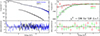 |
Fig. 1. Spectro-polarimetric fit of XMM-Newton (blue) and IXPE I (black), Q (red), and U (green) spectra, with residuals of the best-fit model. Top panels: Best fits to the IXPE and XMM-Newton spectra. Bottom panels: Residuals of the best-fits. Left: Fit of the model tbabs × const × polconst × logpar to the Stokes I spectra. Right: Best-fit Stokes Q and U spectra. |
Spectro-polarimetric best-fit parameters of PKS 2155–304.
The results obtained from the spectro-polarimetric modeling are in agreement with a typical HSP spectrum with α in the range 2.55–2.7 and β = 0.078 ± 0.012. We find that both ΠX and ΨX are significantly constrained, with values of (23.3 ± 1.5)% and 128° ±1.8°, respectively, which is in agreement with Hu et al. (2024). In Figure 2, we show the corresponding confidence regions derived for these two parameters. We do not see significant flux variability during the IXPE pointing (Figure A.2). Nevertheless, we performed the analysis using the IXPE and XMM-Newton datasets separately. We do not find any difference in the derived polarization parameters.
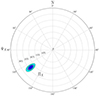 |
Fig. 2. Confidence regions for time-averaged polarization degree (ΠX) and angle (ΨX) obtained from the joint IXPE and XMM-Newton fit. The contours are shown at 68%, 90%, and 99% confidence levels. |
2.5. Time- and energy-resolved analysis
We additionally investigated the possibility of polarization variability over time and energy using the χ2 test for a fit of a constant model to the normalized q = Q/I and u = U/I Stokes parameters, as implemented in Di Gesu et al. (2023) and Kim et al. (2024). We calculated the null-hypothesis probability of the constant model considering the degrees of freedom and χ2 values from the result of each fit. First, time variability was tested by dividing the entire observation period into 2–15 subperiods. For all subdivisions except 11, 13, and 15, we found that the null-hypothesis probability of the u Stokes parameter being constant throughout the observation was < 1%. The lowest null-hypothesis chance probability found was < 0.000127, which occurred when dividing the IXPE pointing into two equal time bins. As shown in Table 2 and Figure 3, during the first period (T1), we obtained ΠX, T1 = (30.7 ± 2.0)% and ΨX, T1 = 129.4° ± 1.8°; while during the second period (T2), we found ΠX, T2 = (15.3 ± 2.1)% and ΨX, T2 = 125.4° ± 3.9°. The polarization angle was essentially stable, within the 1σ uncertainty, from T1 to T2, while the polarization degree varied markedly between the two time bins.
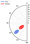 |
Fig. 3. Polarization contours for time periods T1 (blue) and T2 (red), obtained when performing a time-resolved analysis. The contours are shown at confidence levels of 68.27%, 90.00%, and 99.00%. |
Time-resolved IXPE polarization results of PKS 2155−304.
The above time-resolved analysis included data over the entire 2–8 keV IXPE high-sensitivity energy range. We also performed an energy-resolved analysis integrated in time over the entire IXPE pointing. We subdivided the 2–8 keV sensitivity range into multiple energy bins: two 3 keV bins (2–5 keV and 5–8 keV) up to 12 0.5 keV bins (2.0–2.5 keV, …, 7.5–8.0 keV). A χ2 test finds no significant difference in polarization properties across the subdivided energy bins. Additionally, we performed a test where the energy and time are divided simultaneously (T1 with 2–5 keV, T1 with 5–8 keV, T2 with 2–5 keV, and T2 with 5–8 keV); we found that there is no significant difference in polarization properties across the subdivided energy bins within the uncertainty of each polarization measurement.
3. Contemporaneous multiwavelength observations
Contemporaneous to the IXPE observation, PKS 2155–304 was observed in radio and optical bands. Here we provide a brief description of the observations and data analysis procedures. More details about data reduction can be found in Liodakis et al. (2022a) and Di Gesu et al. (2023).
At radio frequencies, observations were provided by the Effelsberg 100-m radio telescope and the Korean VLBI Network (KVN). Effelsberg observations were performed within the QUIVER (monitoring the Stokes Q, U, I, and V emission of AGN jets in radio) program at 4.85, 10.45, and 13.8 GHz. The KVN observations were performed using the Yonsei and Tamna antennas in single-dish mode (Kang et al. 2015) at 25, 43, 86, and 129 GHz. Millimeter-wave radio (mm-radio) observations were provided by the SubMillimeter Array (SMA) polarimeter (Marrone & Rao 2008) within the SMAPOL (SMA Monitoring of AGNs with POLarization) program at 225.5 GHz (Myserlis et al., in prep.).
We have found that the source was weakly polarized across all radio bands. At frequencies lower than 129 GHz, we are only able to obtain upper limits. In the 4.85–13.8 GHz regime, the polarization degree is < 3% (99.7% C.I.). At KVN frequencies, the most constrained upper limit estimate is < 4.4% (99.7% C.I.), found at 43 GHz. At 225.5 GHz, we observed the source on 2023 October 27, November 4, and November 6. The first two observations yielded 99.7% C.I. upper limits of < 2.61% and < 0.81%. In the third observation, we measured the radio (225.5 GHz) polarization degree to be ΠR = (1.7 ± 0.4)%, along a polarization angle of ΨR = 112.5° ±5.5°. The polarization results in the radio band are summarized in Table 3.
Linear polarization results of PKS 2155–304 in the radio bands.
We conducted contemporaneous optical observations at the Calar Alto Observatory using the Calar Alto Faint Object Spectrograph (CAFOS), the 60 cm telescope at Belogradchik Observatory, the Kanata telescope using the Hiroshima Optical and Near-InfraRed camera (HONIR, Kawabata et al. 1999; Akitaya et al. 2014), the Liverpool Telescope using the Multicolour OPTimised Optical Polarimeter (MOPTOP), the Boston University Perkins Telescope Observatory using the PRISM instrument, and the South African Astronomical Observatory using the HIgh-speed Photo-POlarimeter (HIPPO, Potter et al. 2010). HIPPO uses two contra-rotating 1/2 and 1/4 wave-plates and can simultaneously measure linear and circular polarization by fitting the amplitude and phases of the fourth, eighth (linear), and sixth (circular) harmonic (Potter et al. 2008, 2010). The 60 cm telescope at Belogradchik observatory uses a set of three polarizing filters, oriented at 0, 60, and 120 degrees, and standard photometric procedures. Details on the analysis and calibration for these observations can be found in Bachev et al. (2023). MOPTOP features a dual-beam configuration, with a pair of fast-readout, very-low-noise CMOS cameras, and a continuously rotating half-wave plate. These allow for high-sensitivity observations while minimizing systematic errors. MOPTOP has a FOV of 7 × 7 arcsec2 (Shrestha et al. 2020). Quasi-simultaneous observations were taken in filters B (380–520 nm), V (490–570 nm), and R (580–695 nm). The observations were carried out in slow mode with 16 × 4 s integrations per camera being used to calculate four sets of Stokes IQU parameters. These were averaged before calculating the photopolarimetric data for further minimization of the uncertainties. The photometric data were calculated via standard differential photometry techniques with the astropy and photutils packages in Python, using a calibration star with known BVR magnitudes. The polarimetric data were calibrated using zero-polarized and polarized standard stars to characterize the instrumental polarization, position angle, and depolarization values.
In HSP sources, the unpolarized starlight from the host-galaxy has a depolarizing effect on the raw measurements of the optical polarization degree (ΠO). To correct for this, the host-galaxy flux density (Ih) contribution within the aperture used in the polarization measurements is needed. We carefully estimated Ih for different aperture sizes by convolving the known surface brightness measurement of PKS 2155–304 (14.8 R-band magnitudes, equivalent to 3.70 mJy, at an effective radius of 4.5 arcsec; Falomo et al. 1991) to different seeing and subtracting the blazar contribution from it. The modeled host-galaxy magnitude (m) against the aperture radius (r) can be mathematically represented as m = μe − 5log(Re)−2.5log[2πn ⋅ ebn/(bn)2n ⋅ Γ(2n, x)⋅γ(2n)], where x = bn(r/Re)−n, Γ is the incomplete gamma function, and γ is the gamma function (e.g., Graham & Driver 2005). For the host-galaxy of PKS 2155–304, we obtained the fit parameters n = 1.507, bn = 2n − 0.324, Re = 2.87, and μe = 21.03. For example, when using an aperture of 7.5 arcsec in radius, the host-galaxy flux density contribution is 1.27 ± 0.13 mJy in the R band. The intrinsic polarization degree (Πi) is then estimated as Πi = ΠO ⋅ It/(It − Ih), where It is the total flux density (Hovatta et al. 2016). This approach allows for the host-galaxy-correction of all R band polarization measurements that are accompanied by a photometric image. This was performed for several R-band data sets, whose host-galaxy-corrected ΠO2 values are shown in Figure 4, labeled as R band†. We note that the host-galaxy contribution is dependent on the wavelength. For example, the host galaxy is brighter in IR bands, while dimmer in higher energy optical bands. Unfortunately, the aforementioned modeling of the host-galaxy was only possible in the R band. Therefore, we can only correct for the host-galaxy contribution in the R band.
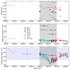 |
Fig. 4. IXPE and contemporaneous multiwavelength polarization of PKS 2155−304. Panels from top to bottom are optical brightness, multiwavelength polarization degree, and multiwavelength polarization angle. The vertical gray shaded area demarcates the duration of the IXPE observation. Horizontal lavender shaded area in the bottom panel denotes the approximate position angle of the extended (> 1.5 pc) VLBI jet (see Sect. 1). The † symbol refers to host-galaxy-corrected values. To calculate ΠX/ΠO, we used the average host-galaxy-corrected ΠO in each of the two IXPE time bins. |
Table 4 summarizes the optical observations of PKS 2155–304. During the IXPE pointing (between MJD 60244 and 60255), we find that ΠO was rather stable, with average host-galaxy-corrected R-band values of (4.3 ± 0.7)% and (3.8 ± 0.9)% for the first and second halves of the pointing, respectively. We measure ΨO to be in the 90°–140° range. We note that while we were only able to perform host-galaxy correction in the R band (which is rather narrow), the host-galaxy contribution in the B and V bands is usually negligible. In the I and J bands the contribution is expected to be greater, which would shift their corrected polarization degrees closer to the corrected R-band values. Due to the high density of data points in the optical and near-IR bands (see Figure 4), in Appendix B (Figure B.1) we plot a zoomed-in view of the light curves to allow for a better analysis of the color-dependent properties of these bands. We find that while ΠO underwent rather achromatic variations, the simultaneous polarization degrees at the B band were consistently higher than those of the host-galaxy-corrected R band, with an average ratio around 1.2 (see Figure B.1). In Appendix B, we additionally visualize the chromatic intra-night variations observed during the IXPE pointing. The polarization angle ΨO exhibited a continuous and achromatic rotation from ∼140° to ∼90° between MJD 60244 and 60251, after which the value increased to ∼130° (at MJD 60257 and staying roughly the same during the following three nights). While the average source brightness differed strongly with color in the optical bands, with the source being brighter in the redder bands due to stronger host-galaxy contamination, the time-resolved brightness of all the colors showed little variability during the IXPE pointing. Overall, these values were comparable to the typical ones seen in the decade-long monitoring results of PKS 2155−304 at Steward Observatory (see Appendix A), indicating that the source was in an average optical state when IXPE observed it. We note that ΠO was a factor of ∼2 greater than the polarization degree in the radio band (ΠR) and ΨO was consistent with the simultaneous radio band polarization angle (ΨR; see Figure 4).
Linear polarization results of PKS 2155–304 in the optical and near-IR bands.
Optical (R-band) circular polarization observations of the source using HIPPO yielded an upper limit of < 0.87% at 99.7% C.I. during the IXPE observation.
4. Discussion
Several particle acceleration mechanisms have been suggested to explain how electron populations in HSP blazar jets can reach the energies needed for their synchrotron luminosity to peak in the X-ray regime. Diffusive shock acceleration in weakly magnetized jets is one such mechanism (e.g., Blandford & Eichler 1987). For example, Marscher (2014) considered a scenario where a conical standing shock energizes turbulent plasma as it crosses the shock front, with some regions being accelerated more effectively due to favorable orientation of their magnetic field lines relative to the front. The particles lose energy by radiating as they advect farther from the shock; hence, there is a gradient in maximum particle energy in the emitting region. This multi-zone emission model can explain the general nature of temporal variations observed in the flux and polarization. In the case of an HSP blazar, this model predicts a higher mean value of ΠX with higher-amplitude variations than at longer wavelengths (Marscher & Jorstad 2022; Peirson & Romani 2018). It additionally predicts random rotations of Ψ with varying rate, magnitude ΔΨ, and direction (clockwise or counterclockwise).
Particle acceleration in a shock or compressed plasmoid moving down a jet with a partially ordered or helical magnetic field has also been suggested (e.g., Blandford & Königl 1979; Marscher & Gear 1985; Sikora et al. 1994; Marscher et al. 2008). If the plasmoid has uniform physical conditions, the multifrequency emission is co-spatial, hence the polarization patterns across different frequencies are expected to be similar (Di Gesu et al. 2022b). In contrast, a moving shock should have similar multiwavelength properties as described above for a standing shock, with stratification of the maximum-energy (and therefore frequency) profile. The volume occupied by the lower-energy particles is greater, hence vector averaging of the disordered, or otherwise multidirectional, magnetic field lowers the polarization at longer wavelengths. This leads to wavelength dependence of Π, whose mean value is expected to decrease toward longer wavelengths (e.g., Angelakis et al. 2016; Tavecchio et al. 2018). Furthermore, as the flow crosses the shock front, the component of the internal magnetic field that is parallel to the shock front becomes more ordered, which results in Ψ at the synchrotron peak frequency (ΨX for HSP blazars) aligning with the jet direction. In the case of a helically twisted magnetic field structure in the jet (evidence for which is found in parsec-scale VLBI observations; e.g., Hovatta et al. 2012), Ψ at the synchrotron SED peak frequency is expected to exhibit non-stochastic rotations resulting from the passage of the shock front through the jet. In blazars whose SED peaks in the optical regime, systematic ΨO rotations have been observed, with some being temporally correlated with GeV γ-ray flares (Blinov et al. 2015, 2018). Additionally, a harder-when-brighter spectral behavior can be expected in the case of shock-front acceleration (Kirk et al. 1998).
If the jets are highly magnetized, shock acceleration is not effective. Instead, magnetic reconnection could efficiently convert magnetic energy into particle energy (Sironi & Spitkovsky 2014; Sironi et al. 2015). For example, this can involve current sheets generated by kink instabilities (Bodo et al. 2021). Further stochastic acceleration can follow the injection of particles into turbulent regions (Comisso & Sironi 2018). The expected observed polarization resulting from magnetic reconnection scenarios, averaged over the IXPE ∼ 10–100 ks integration times, would correspond to ΠX ≲ ΠO and a different temporal evolution for ΨX than ΨO (Di Gesu et al. 2022b).
Alternatively, Zhang et al. (2020) considered a striped-jet scenario where more antiparallel magnetic-field lines are expected to form than in the kink instability and turbulent scenarios, leading to the production, merger, and acceleration of plasmoids. Their observational predictions include a harder-when-brighter behavior and more temporal variability of ΠX than ΠO as ΨX undergoes significant 90°–180° rotations along the anti-parallel field lines. Integrated over an IXPE pointing, this is expected to yield ΠX < ΠO.
In the case of PKS 2155–304, we find that Ψ at all wavelengths is in the general direction of the parsec-scale jet seen in the VLBI images (which is generally southeast at ∼135°; see Sect. 1). Our single significant radio detection of polarization measured ΨR∼110°, which is roughly aligned with the jet direction. In the X-ray band, we find no evidence that ΨX changed during the IXPE pointing, while in the optical band it rotated from ΨO∼140° at the beginning to ∼90° at around MJD 60251, then up to ∼100° at the end of the IXPE pointing, and further up to ∼130° at MJD 60257. We note that such ∼ ± 25° fluctuations with a mean value of ΨO are typical of PKS 2155–304, as tracked by Steward Observatory (see Appendix A). However, the mean value gradually drifted from ∼80° to ∼40° in around ten years, ending in 2020. This is quite different in both the rate and range of values from the rotation on a timescale of days seen in our data set, throughout which Ψ at all wavelengths is roughly aligned with the VLBI jet direction. This is a strong indication of particle acceleration occurring in regions with a magnetic field predominantly oriented orthogonally to the jet axis, as expected in the shock acceleration scenario or for a jet with a dominant toroidal field. Additionally, the discrepant behavior between ΨX and ΨO indicates that at least part of their emission arises in separate regions in the jet. Furthermore, the lack of evidence for any fast changes in Ψ strongly disfavors particle-acceleration mechanisms resulting from magnetic reconnection or large-scale turbulence.
Regarding the polarization degree, we find that ΠX > ΠO > ΠR held true throughout the IXPE pointing, with ΠX/ΠO being ∼7.2 and ∼4.0 in the first and second halves of the pointing, respectively (see Figure 4). The former (during T1) is the most extreme X-ray-to-optical polarization degree ratio found in a blazar to date, as seen in Figure 5 (also see Figure 6): more than twice that measured for Mrk 421, Mrk 501, and 1ES 1959+650. Moreover, we note that PKS 2155–304 has historically had the softest X-ray spectrum as compared with the others (according to the ROSAT all-sky survey; Boller et al. 2016), which held true during the IXPE pointing. A softer X-ray spectrum is indicative of the X-ray emission originating farther above the synchrotron peak frequency. The particles radiating at X-ray energies in PKS 2155–304 have shorter cooling times and therefore occupy smaller volumes than in the other HSP blazars, according to our interpretation. Emission from such particles would result in a higher mean value – as well as higher-amplitude variability – of ΠX, as the averaging effects due to randomly oriented magnetic fields would be reduced (Peirson et al. 2023). On the other hand, being farther above the synchrotron peak frequency may result in contribution by the high-energy component of the SED in the 2–8 keV band (e.g., Madejski et al. 2016). If that contribution is significant, it may result in somewhat underestimating the measured ΠX.
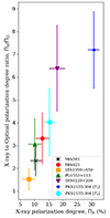 |
Fig. 5. X-ray-to-optical polarization degree ratio (ΠX/ΠO) of the six HSP blazars observed by IXPE plotted against their X-ray polarization degree (ΠX). In the case of PKS 2155−304, the two time bins (T1 and T2) are presented separately (see Sect. 2.5), while for the others the detected (> 99.7% confidence) values are averaged over the IXPE pointing. |
Interestingly, the more polarized-at-higher-frequencies behavior, observed when comparing the X-ray to the optical band results, also occurred within the optical band: the average ratio of the simultaneous B-band to host-galaxy-corrected R-band polarization degrees was 1.2 (see Appendix B). As discussed above and more extensively in Liodakis et al. (2022a) and Di Gesu et al. (2022b), for example, this behavior is expected in the scenario where a compact shock front accelerates particles and partially orders the magnetic field. However, the ratio is substantially larger than predicted by the basic model (see Appendix B).
Notably, we find that, while there were no temporal variations in the optical polarization degree ΠO, there was a significant drop in the X-ray polarization degree ΠX during the IXPE pointing. This reaffirms that the X-ray and longer-wavelength emissions at least partly arose from different regions of the jet. It also indicates that the magnetic field in the X-ray emission region became significantly more disordered over a few days, despite its average orientation remaining constant, as indicated by the constant polarization angle. The X-ray flux also remained steady within the uncertainties (see Appendix A). Such a decrease in order of the magnetic field lines could be caused by a significant strengthening of turbulence in the close vicinity of the shock front (where the high-energy electrons emitting in the X-ray band lose their energy; Angelakis et al. 2016). As discussed in Liodakis et al. (2022a) and Marscher & Jorstad (2022), the polarization of the turbulent component of the field is expected to vary with an amplitude equal to the square-root of the mean polarization degree. While this could explain the change in ΠX from T1 to T2, a strong variation of ΨX would also be expected, but was not observed. Instead, as mentioned above, the emission region during T1 may have been relatively small (i.e., a few acceleration zones were dominating) resulting in a high value of ΠX. If more acceleration zones were boosted into the emission range detectable by IXPE, then a drop in the mean ΠX during T2 would be expected.
Alternatively, in the framework of the stratified shock model of Tavecchio et al. (2018), a lower polarization degree can be related either to a more rapid decay of the partially ordered magnetic field with distance from the shock (related to the microphysics of the shock) or by a strengthening of the poloidal field carried by the pre-shocked plasma. Detailed modeling of the multiwavelength data is required to extract more precise information and to effectively test the different theoretical scenarios.
To demonstrate the similarity of the radio through X-ray polarization behavior of the six HSP targets observed by IXPE thus far, we plot their average polarization degree (Π) at each general wave band from multiwavelength observations in Figure 6. It is apparent that, on average, ΠX is several times greater than ΠO, which is a natural prediction of the energy-stratified shock-acceleration scenario. If this scenario is at play, then the fairly good agreement between the lower energy multiwavelength polarization degrees (⟨ΠO⟩ and ⟨ΠR⟩) over the different HSP blazars implies that, at a given frequency, their emission regions have similar sizes as well as similar structures and ordering of the magnetic field. However, the significant scatter in the observed X-ray polarization degree (⟨ΠX⟩) of the HSP blazars suggests that shock properties may be prone to greater variability at higher energies.
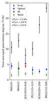 |
Fig. 6. Multiwavelength time-averaged polarization degree of HSP blazars observed by IXPE. Only polarization detections (> 99.7% confidence) were used to calculate the Π time averages. |
5. Conclusions
The IXPE observations of PKS 2155–304 have revealed the highest X-ray polarization yet detected among the six similarly observed HSP blazars. During the ∼10-day IXPE pointing, the X-ray polarization degree (ΠX) decreased from ∼30% during the first half to ∼15% during the second half. Meanwhile, the optical polarization degree (ΠO) remained stable at ∼4%. The X-ray-to-optical ratios of ∼7 and ∼4 in the first and second halves, respectively, are similar to the previous results obtained for HSP blazars (summarized in Figure 6). This consistency disfavors reconnection-based and stochastic turbulent (second-order Fermi) mechanisms for explaining the high energies of particles needed to produce X-ray synchrotron emission in HSP blazars.
During the IXPE pointing, the polarization angle (Ψ) of PKS 2155–304 at all monitored wavelengths was roughly aligned with the direction of the parsec-scale jet. This general alignment of the multiwavelength Ψ with the jet direction indicates that the magnetic field in the particle acceleration region was partially ordered along a direction transverse to the jet. While the X-ray polarization angle remained stable during the IXPE exposure, a clear change in the optical polarization angle was observed. This, combined with the lack of temporal correlation between ΠX and ΠO, suggests that the X-ray and optical emission regions are not completely co-spatial. These findings, well in line with those of previous studies of HSP polarization involving IXPE, can be qualitatively explained by the energy-stratified shock-acceleration scenario. However, the observations executed thus far have sampled only a small range of time intervals, leaving the temporal behavior of the X-ray polarization rather poorly studied. Future X-ray and multiwavelength polarization measurements of HSP blazars are needed in order to determine whether the particle acceleration and other physical characteristics change with time.
Current technology to measure X-ray polarization does not permit measurements of the circular polarization component (Stokes V). Nevertheless, intrinsic circular polarization in blazars should be low (≪1%), and it has yet to be detected with certainty (Liodakis et al. 2022b, 2023).
Throughout this paper, the subscripts O and R refer to the generic optical (including near-IR) and radio bands, respectively. Any filter-specific information then follows the generic subscript in parentheses.
Acknowledgments
The Imaging X-ray Polarimetry Explorer (IXPE) is a joint US and Italian mission. The US contribution is supported by the National Aeronautics and Space Administration (NASA) and led and managed by its Marshall Space Flight Center (MSFC), with industry partner Ball Aerospace (contract NNM15AA18C). The Italian contribution is supported by the Italian Space Agency (Agenzia Spaziale Italiana, ASI) through contract ASI-OHBI-2017-12-I.0, agreements ASI-INAF-2017-12-H0 and ASI-INFN-2017.13-H0, and its Space Science Data Center (SSDC), and by the Istituto Nazionale di Astrofisica (INAF) and the Istituto Nazionale di Fisica Nucleare (INFN) in Italy. This research used data products provided by the IXPE Team (MSFC, SSDC, INAF, and INFN) and distributed with additional software tools by the High-Energy Astrophysics Science Archive Research Center (HEASARC), at NASA Goddard Space Flight Center (GSFC). This work has been partially supported by the ASI-INAF program I/004/11/4. The IAA-CSIC co-authors acknowledge financial support from the Spanish "Ministerio de Ciencia e Innovación" (MCIN/AEI/ 10.13039/501100011033) through the Center of Excellence Severo Ochoa award for the Instituto de Astrofíisica de Andalucía-CSIC (CEX2021-001131-S), and through grants PID2019-107847RB-C44 and PID2022-139117NB-C44. The Submillimetre Array is a joint project between the Smithsonian Astrophysical Observatory and the Academia Sinica Institute of Astronomy and Astrophysics and is funded by the Smithsonian Institution and the Academia Sinica. Mauna Kea, the location of the SMA, is a culturally important site for the indigenous Hawaiian people; we are privileged to study the cosmos from its summit. E.L. was supported by Academy of Finland projects 317636 and 320045. The research at Boston University was supported in part by National Science Foundation grant AST-2108622, NASA Fermi Guest Investigator grant 80NSSC23K1507, and NASA Swift Guest Investigator grant 80NSSC23K1145. The Perkins Telescope Observatory, located in Flagstaff, AZ, USA, is owned and operated by Boston University. I.L was funded by the European Union ERC-2022-STG - BOOTES - 101076343. Views and opinions expressed are however those of the author(s) only and do not necessarily reflect those of the European Union or the European Research Council Executive Agency. Neither the European Union nor the granting authority can be held responsible for them. Some of the data are based on observations collected at the Centro Astronómico Hispano en Andalucía (CAHA), operated jointly by Junta de Andalucía and Consejo Superior de Investigaciones Científicas (IAA-CSIC). This work was supported by NSF grant AST-2109127. We acknowledge the use of public data from the Swift data archive. Based on observations obtained with XMM-Newton, an ESA science mission with instruments and contributions directly funded by ESA Member States and NASA. Partly based on observations with the 100-m telescope of the MPIfR (Max-Planck-Institut für Radioastronomie) at Effelsberg. Observations with the 100-m radio telescope at Effelsberg have received funding from the European Union’s Horizon 2020 research and innovation programme under grant agreement No 101004719 (ORP). I.L was supported by the NASA Postdoctoral Program at the Marshall Space Flight Center, administered by Oak Ridge Associated Universities under contract with NASA. S. Kang, S.-S. Lee, W. Y. Cheong, S.-H. Kim, and H.-W. Jeong were supported by the National Research Foundation of Korea (NRF) grant funded by the Korea government (MIST) (2020R1A2C2009003). The KVN is a facility operated by the Korea Astronomy and Space Science Institute. The KVN operations are supported by KREONET (Korea Research Environment Open NETwork) which is managed and operated by KISTI (Korea Institute of Science and Technology Information). This work was supported by JST, the establishment of university fellowships towards the creation of science technology innovation, Grant Number JPMJFS2129. This work was supported by Japan Society for the Promotion of Science (JSPS) KAKENHI Grant Numbers JP21H01137. This work was also partially supported by Optical and Near-Infrared Astronomy Inter-University Cooperation Program from the Ministry of Education, Culture, Sports, Science and Technology (MEXT) of Japan. We are grateful to the observation and operating members of Kanata Telescope. Data from the Steward Observatory spectropolarimetric monitoring project were used. This program is supported by Fermi Guest Investigator grants NNX08AW56G, NNX09AU10G, NNX12AO93G, and NNX15AU81G. This research was partially supported by the Bulgarian National Science Fund of the Ministry of Education and Science under grants KP-06-H38/4 (2019) and KP-06-PN-68/1 (2022). The Liverpool Telescope is operated on the island of La Palma by Liverpool John Moores University in the Spanish Observatorio del Roque de los Muchachos of the Instituto de Astrofisica de Canarias with financial support from the UKRI Science and Technology Facilities Council (STFC) (ST/T00147X/1). We thank Talvikki Hovatta for fruitful discussion about the VLBI images.
References
- Aharonian, F., Akhperjanian, A. G., Bazer-Bachi, A. R., et al. 2005, A&A, 442, 895 [NASA ADS] [CrossRef] [EDP Sciences] [Google Scholar]
- Aharonian, F., Akhperjanian, A. G., Bazer-Bachi, A. R., et al. 2007, ApJ, 664, L71 [NASA ADS] [CrossRef] [Google Scholar]
- Aharonian, F., Akhperjanian, A. G., Anton, G., et al. 2009, ApJ, 696, L150 [NASA ADS] [CrossRef] [Google Scholar]
- Akitaya, H., Moritani, Y., Ui, T., et al. 2014, SPIE Conf. Ser., 9147, 91474O [NASA ADS] [Google Scholar]
- Angelakis, E., Hovatta, T., Blinov, D., et al. 2016, MNRAS, 463, 3365 [NASA ADS] [CrossRef] [Google Scholar]
- Arnaud, K. A. 1996, ASP Conf. Ser., 101, 17 [Google Scholar]
- Bachev, R., Tripathi, T., Gupta, A. C., et al. 2023, MNRAS, 522, 3018 [NASA ADS] [CrossRef] [Google Scholar]
- Blandford, R., & Eichler, D. 1987, Phys. Rep., 154, 1 [Google Scholar]
- Blandford, R. D., & Königl, A. 1979, ApJ, 232, 34 [Google Scholar]
- Blandford, R., Meier, D., & Readhead, A. 2019, ARA&A, 57, 467 [NASA ADS] [CrossRef] [Google Scholar]
- Blinov, D., Pavlidou, V., Papadakis, I., et al. 2015, MNRAS, 453, 1669 [NASA ADS] [CrossRef] [Google Scholar]
- Blinov, D., Pavlidou, V., Papadakis, I., et al. 2018, MNRAS, 474, 1296 [CrossRef] [Google Scholar]
- Bodo, G., Tavecchio, F., & Sironi, L. 2021, MNRAS, 501, 2836 [NASA ADS] [CrossRef] [Google Scholar]
- Boller, T., Freyberg, M. J., Trümper, J., et al. 2016, A&A, 588, A103 [NASA ADS] [CrossRef] [EDP Sciences] [Google Scholar]
- Bowyer, S., Brodie, J., Clarke, J. T., & Henry, J. P. 1984, ApJ, 278, L103 [NASA ADS] [CrossRef] [Google Scholar]
- Burrows, D. N., Hill, J. E., Nousek, J. A., et al. 2005, Space Sci. Rev., 120, 165 [Google Scholar]
- Carini, M. T., & Miller, H. R. 1992, ApJ, 385, 146 [Google Scholar]
- Comisso, L., & Sironi, L. 2018, Phys. Rev. Lett., 121, 255101 [NASA ADS] [CrossRef] [Google Scholar]
- Di Gesu, L., Donnarumma, I., Tavecchio, F., et al. 2022a, ApJ, 938, L7 [CrossRef] [Google Scholar]
- Di Gesu, L., Tavecchio, F., Donnarumma, I., et al. 2022b, A&A, 662, A83 [NASA ADS] [CrossRef] [EDP Sciences] [Google Scholar]
- Di Gesu, L., Marshall, H. L., Ehlert, S. R., et al. 2023, Nat. Astron., 7, 1245 [NASA ADS] [CrossRef] [Google Scholar]
- Ehlert, S. R., Ferrazzoli, R., Marinucci, A., et al. 2022, ApJ, 935, 116 [NASA ADS] [CrossRef] [Google Scholar]
- Ehlert, S. R., Liodakis, I., Middei, R., et al. 2023, ApJ, 959, 61 [NASA ADS] [CrossRef] [Google Scholar]
- Errando, M., Liodakis, I., Marscher, A. P., et al. 2024, ApJ, 963, 5 [NASA ADS] [CrossRef] [Google Scholar]
- Falomo, R., Giraud, E., Maraschi, L., et al. 1991, ApJ, 380, L67 [NASA ADS] [CrossRef] [Google Scholar]
- Georganopoulos, M., & Kazanas, D. 2003, ApJ, 594, L27 [NASA ADS] [CrossRef] [Google Scholar]
- Ghisellini, G., Tavecchio, F., & Chiaberge, M. 2005, A&A, 432, 401 [CrossRef] [EDP Sciences] [Google Scholar]
- Giannios, D., Uzdensky, D. A., & Begelman, M. C. 2009, MNRAS, 395, L29 [NASA ADS] [CrossRef] [Google Scholar]
- Giommi, P., Perri, M., Capalbi, M., et al. 2021, MNRAS, 507, 5690 [NASA ADS] [CrossRef] [Google Scholar]
- Graham, A. W., & Driver, S. P. 2005, PASA, 22, 118 [NASA ADS] [CrossRef] [Google Scholar]
- Griffiths, R. E., Tapia, S., Briel, U., & Chaisson, L. 1979, ApJ, 234, 810 [NASA ADS] [CrossRef] [Google Scholar]
- H.E.S.S. Collaboration (Abramowski, A., et al.) 2012, A&A, 539, A149 [NASA ADS] [CrossRef] [EDP Sciences] [Google Scholar]
- HI4PI Collaboration (Ben Bekhti, N., et al.) 2016, A&A, 594, A116 [NASA ADS] [CrossRef] [EDP Sciences] [Google Scholar]
- Hovatta, T., & Lindfors, E. 2019, New Astron Rev., 87, 101541 [NASA ADS] [CrossRef] [Google Scholar]
- Hovatta, T., Lister, M. L., Aller, M. F., et al. 2012, AJ, 144, 105 [Google Scholar]
- Hovatta, T., Lindfors, E., Blinov, D., et al. 2016, A&A, 596, A78 [NASA ADS] [CrossRef] [EDP Sciences] [Google Scholar]
- Hu, X.-K., Yu, Y.-W., Zhang, J., et al. 2024, ApJ, 963, L41 [NASA ADS] [CrossRef] [Google Scholar]
- Jansen, F., Lumb, D., Altieri, B., et al. 2001, A&A, 365, L1 [NASA ADS] [CrossRef] [EDP Sciences] [Google Scholar]
- Kang, S., Lee, S.-S., & Byun, D.-Y. 2015, J. Korean Astron. Soc., 48, 257 [NASA ADS] [CrossRef] [Google Scholar]
- Kawabata, K. S., Okazaki, A., Akitaya, H., et al. 1999, PASP, 111, 898 [NASA ADS] [CrossRef] [Google Scholar]
- Kim, D. E., Di Gesu, L., Liodakis, I., et al. 2024, A&A, 681, A12 [NASA ADS] [CrossRef] [EDP Sciences] [Google Scholar]
- Kirk, J. G., Rieger, F. M., & Mastichiadis, A. 1998, A&A, 333, 452 [NASA ADS] [Google Scholar]
- Lico, R., Liu, J., Giroletti, M., et al. 2020, A&A, 634, A87 [NASA ADS] [CrossRef] [EDP Sciences] [Google Scholar]
- Liodakis, I., Marscher, A. P., Agudo, I., et al. 2022a, Nature, 611, 677 [CrossRef] [Google Scholar]
- Liodakis, I., Blinov, D., Potter, S. B., & Rieger, F. M. 2022b, MNRAS, 509, L21 [Google Scholar]
- Liodakis, I., Shablovinskaya, E., Blinov, D., et al. 2023, A&A, 680, L11 [NASA ADS] [CrossRef] [EDP Sciences] [Google Scholar]
- Madejski, G. M., Nalewajko, K., Madsen, K. K., et al. 2016, ApJ, 831, 142 [NASA ADS] [CrossRef] [Google Scholar]
- Marrone, D. P., & Rao, R. 2008, SPIE Conf. Ser., 7020, 70202B [NASA ADS] [Google Scholar]
- Marscher, A. P. 2014, ApJ, 780, 87 [Google Scholar]
- Marscher, A. P., & Gear, W. K. 1985, ApJ, 298, 114 [Google Scholar]
- Marscher, A. P., & Jorstad, S. G. 2021, Galaxies, 9, 27 [NASA ADS] [CrossRef] [Google Scholar]
- Marscher, A. P., & Jorstad, S. G. 2022, Universe, 8, 644 [NASA ADS] [CrossRef] [Google Scholar]
- Marscher, A. P., Jorstad, S. G., D’Arcangelo, F. D., et al. 2008, Nature, 452, 966 [Google Scholar]
- Massaro, E., Perri, M., Giommi, P., & Nesci, R. 2004, A&A, 413, 489 [NASA ADS] [CrossRef] [EDP Sciences] [Google Scholar]
- Middei, R., Marinucci, A., Braito, V., et al. 2022a, MNRAS, 514, 2974 [NASA ADS] [CrossRef] [Google Scholar]
- Middei, R., Giommi, P., Perri, M., et al. 2022b, MNRAS, 514, 3179 [NASA ADS] [CrossRef] [Google Scholar]
- Middei, R., Perri, M., Puccetti, S., et al. 2023, ApJ, 953, L28 [NASA ADS] [CrossRef] [Google Scholar]
- Paliya, V. S., Zhang, H., Böttcher, M., et al. 2018, ApJ, 863, 98 [Google Scholar]
- Peirson, A. L., & Romani, R. W. 2018, ApJ, 864, 140 [NASA ADS] [CrossRef] [Google Scholar]
- Peirson, A. L., Negro, M., Liodakis, I., et al. 2023, ApJ, 948, L25 [NASA ADS] [CrossRef] [Google Scholar]
- Piner, B. G., & Edwards, P. G. 2004, ApJ, 600, 115 [Google Scholar]
- Piner, B. G., Pant, N., & Edwards, P. G. 2008, ApJ, 678, 64 [Google Scholar]
- Piner, B. G., Pant, N., & Edwards, P. G. 2010, ApJ, 723, 1150 [Google Scholar]
- Potter, S., Buckley, D., O’Donoghue, D., et al. 2008, SPIE Conf. Ser., 7014, 70145E [NASA ADS] [Google Scholar]
- Potter, S. B., Buckley, D. A. H., O’Donoghue, D., et al. 2010, MNRAS, 402, 1161 [CrossRef] [Google Scholar]
- Schwartz, D. A., Doxsey, R. E., Griffiths, R. E., Johnston, M. D., & Schwarz, J. 1979, ApJ, 229, L53 [Google Scholar]
- Shrestha, M., Steele, I. A., Piascik, A. S., et al. 2020, MNRAS, 494, 4676 [NASA ADS] [CrossRef] [Google Scholar]
- Sikora, M., Begelman, M. C., & Rees, M. J. 1994, ApJ, 421, 153 [Google Scholar]
- Sironi, L., & Spitkovsky, A. 2014, ApJ, 783, L21 [NASA ADS] [CrossRef] [Google Scholar]
- Sironi, L., Petropoulou, M., & Giannios, D. 2015, MNRAS, 450, 183 [Google Scholar]
- Smith, P. S., Montiel, E., Rightley, S., et al. 2009, arXiv e-prints [arXiv:0912.3621] [Google Scholar]
- Strüder, L., Briel, U., Dennerl, K., et al. 2001, A&A, 365, L18 [Google Scholar]
- Tavecchio, F., Landoni, M., Sironi, L., & Coppi, P. 2018, MNRAS, 480, 2872 [NASA ADS] [CrossRef] [Google Scholar]
- Weaver, Z. R., Jorstad, S. G., Marscher, A. P., et al. 2022, ApJS, 260, 12 [NASA ADS] [CrossRef] [Google Scholar]
- Weisskopf, M. C., Soffitta, P., Baldini, L., et al. 2022, J. Astron. Telesc. Instrum. Syst., 8, 026002 [NASA ADS] [CrossRef] [Google Scholar]
- Zhang, H., Li, X., Giannios, D., et al. 2020, ApJ, 901, 149 [CrossRef] [Google Scholar]
Appendix A: Long-term variability of PKS 2155–304
It is interesting to place the behavior of PKS 2155–304 during the IXPE pointing in the context of the longer-term variations. In Figure A.1, we present the light curve from ten years of optical polarization monitoring at Steward observatory (Smith et al. 2009). Additionally, in Figure A.2, we present the two-month-long X-ray flux versus time as measured by Swift-XRT (see §2.3).
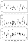 |
Fig. A.1. Decade-long flux and polarization monitoring of PKS 2155−304 in the optical band at Steward observatory (Smith et al. 2009). Top: Brightness in magnitudes. Middle: Polarization degree. Bottom: Polarization angle. |
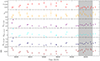 |
Fig. A.2. Two-month-long Swift-XRT X-ray light curve of PKS 2155−304. The best-fit parameters of the logarithmic parabola spectral model, as well as the X-ray fluxes (in the units: 10−11 erg cm−2 s−1) in different bands and their ratios (0.5-2/2-10), are shown as a function of time. The gray shaded area identifies epochs of the IXPE observation. PKS 2155−304 was in an average X-ray flux state during the IXPE pointing. |
The Steward optical data clearly show that the average flux state of the source in the V band is between 13 and 14 magnitudes. It additionally shows that the optical polarization degree (measured in the wavelength range of 500–700 nm) typically varies between 2% and 10%, while its polarization angle seems to generally vary between 60° and 120°. The observed optical brightness and polarization properties of PKS 2155−304 during the IXPE pointing fall well in line with these typical values (see §3). This implies that the source was in an average optical state when IXPE observed it. Likewise, the two-month Swift-XRT data, although much shorter than ten years, suggests that PKS 2155–304 was also in an average flux state in the X-ray band.
Appendix B: Detailed optical and near-IR light curves of PKS 2155–304
The light curves of the optical and near-IR brightness, polarization degree, and polarization angle of PKS 2155–304 are plotted in Figure B.1, which provides a zoomed-in version of Figure 6. The polarization properties are averaged within bins that are separated by the daily optical gaps. Additionally, to show the level of intra-night variability in the optical and near-IR bands, in Figure B.2 we zoom in (without performing any temporal rebinning) on three example nights with good time coverage, namely MJDs 60245, 60247, and 60248.
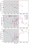 |
Fig. B.1. Optical and near-IR light curves of PKS 2155−304 during and after the IXPE pointing. Using the largest daily gaps, we binned the data points of each filter. We note that only some of the optical R-band data points are host-galaxy-corrected, and these are labeled as R†. The average, simultaneous ratio of the polarization degree of the B-band (380–520 nm, i.e., 2.4–3.3 eV), ΠO(B), to the polarization degree of the host-galaxy-corrected R-band (580–695 nm, i.e., 1.8–2.1 eV), ΠO(R†), is around 1.2 ± 0.2. The gray shaded area shows the IXPE pointing time window. Top: Brightness in magnitudes. Middle: Polarization degree. Bottom: Polarization angle. |
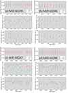 |
Fig. B.2. Zoomed-in optical and near-IR light curves of PKS 2155−304 on the four indicated example nights. The red data points (R†) are those of the host-galaxy-corrected optical R-band, and the cyan ones are those of the near-IR J-band (not host-galaxy-corrected). |
Figure B.1 shows that, during the IXPE pointing, the optical brightness behavior was chromatic, with higher fluxes at longer wavelength bands. Although this could be partly caused by the unknown-host-galaxy contributions, especially in the case of the near-IR bands for which the host contamination is expected to be most prominent, it is normal for the flux to be an increasing function of wavelength in blazars. Otherwise, we find that the optical and near-IR band polarization properties varied rather achromatically. However, the polarization degree at the B band, ΠO(B), was consistently greater than that of the host-galaxy-corrected R band, ΠO(R†). Measuring  for simultaneous data points and averaging its value results in 1.2 ± 0.2. To compare this ratio to a theoretical prediction, we used the turbulence-plus-shock model that theoretically predicts the average polarization degree to be < Π> ≈
  , where ford refers to the fraction of the magnetic field that is well ordered, and N(λ) refers to the number of turbulent cells as a function of wavelength, λ, which can be estimated as N(λ)∝λ1/2 (Marscher & Jorstad 2022). For the two optical bands, R (median wavelength of 640 nm) and B (450 nm), we find NB/NR ≈ 0.8. Assuming ford ≈ 0.05 and NR ≈ 1000 for the R band, as estimated by Marscher & Jorstad (2022), we derive < ΠO(R)> ≈ 4.4%. In the case of the B band, where NB is estimated to be around 1000 × 0.8 = 800, we obtain < ΠO(R)> ≈ 4.5%. Therefore, the theoretical model results in
  ≈ 1.03. Although this is much smaller than the measured ratio, it is still compatible with the observed value within the estimated uncertainty. If such a discrepancy is shown to be statistically significant with future high-cadence optical polarization observations of HSP blazars, it would signal an underlying discrepancy with the turbulence-plus-shock model.
Figure B.2 shows clear signs of intra-night variability in the optical band of PKS 2155−304. Although a detailed analysis of these is beyond the scope of this paper, such densely sampled optical polarization light curves can be instrumental in understanding the underlying mechanisms at play in blazar jets (e.g., Marscher & Jorstad 2021).
All Tables
All Figures
|
Fig. 1. Spectro-polarimetric fit of XMM-Newton (blue) and IXPE I (black), Q (red), and U (green) spectra, with residuals of the best-fit model. Top panels: Best fits to the IXPE and XMM-Newton spectra. Bottom panels: Residuals of the best-fits. Left: Fit of the model tbabs × const × polconst × logpar to the Stokes I spectra. Right: Best-fit Stokes Q and U spectra. |
| In the text | |
|
Fig. 2. Confidence regions for time-averaged polarization degree (ΠX) and angle (ΨX) obtained from the joint IXPE and XMM-Newton fit. The contours are shown at 68%, 90%, and 99% confidence levels. |
| In the text | |
|
Fig. 3. Polarization contours for time periods T1 (blue) and T2 (red), obtained when performing a time-resolved analysis. The contours are shown at confidence levels of 68.27%, 90.00%, and 99.00%. |
| In the text | |
|
Fig. 4. IXPE and contemporaneous multiwavelength polarization of PKS 2155−304. Panels from top to bottom are optical brightness, multiwavelength polarization degree, and multiwavelength polarization angle. The vertical gray shaded area demarcates the duration of the IXPE observation. Horizontal lavender shaded area in the bottom panel denotes the approximate position angle of the extended (> 1.5 pc) VLBI jet (see Sect. 1). The † symbol refers to host-galaxy-corrected values. To calculate ΠX/ΠO, we used the average host-galaxy-corrected ΠO in each of the two IXPE time bins. |
| In the text | |
|
Fig. 5. X-ray-to-optical polarization degree ratio (ΠX/ΠO) of the six HSP blazars observed by IXPE plotted against their X-ray polarization degree (ΠX). In the case of PKS 2155−304, the two time bins (T1 and T2) are presented separately (see Sect. 2.5), while for the others the detected (> 99.7% confidence) values are averaged over the IXPE pointing. |
| In the text | |
|
Fig. 6. Multiwavelength time-averaged polarization degree of HSP blazars observed by IXPE. Only polarization detections (> 99.7% confidence) were used to calculate the Π time averages. |
| In the text | |
|
Fig. A.1. Decade-long flux and polarization monitoring of PKS 2155−304 in the optical band at Steward observatory (Smith et al. 2009). Top: Brightness in magnitudes. Middle: Polarization degree. Bottom: Polarization angle. |
| In the text | |
|
Fig. A.2. Two-month-long Swift-XRT X-ray light curve of PKS 2155−304. The best-fit parameters of the logarithmic parabola spectral model, as well as the X-ray fluxes (in the units: 10−11 erg cm−2 s−1) in different bands and their ratios (0.5-2/2-10), are shown as a function of time. The gray shaded area identifies epochs of the IXPE observation. PKS 2155−304 was in an average X-ray flux state during the IXPE pointing. |
| In the text | |
|
Fig. B.1. Optical and near-IR light curves of PKS 2155−304 during and after the IXPE pointing. Using the largest daily gaps, we binned the data points of each filter. We note that only some of the optical R-band data points are host-galaxy-corrected, and these are labeled as R†. The average, simultaneous ratio of the polarization degree of the B-band (380–520 nm, i.e., 2.4–3.3 eV), ΠO(B), to the polarization degree of the host-galaxy-corrected R-band (580–695 nm, i.e., 1.8–2.1 eV), ΠO(R†), is around 1.2 ± 0.2. The gray shaded area shows the IXPE pointing time window. Top: Brightness in magnitudes. Middle: Polarization degree. Bottom: Polarization angle. |
| In the text | |
|
Fig. B.2. Zoomed-in optical and near-IR light curves of PKS 2155−304 on the four indicated example nights. The red data points (R†) are those of the host-galaxy-corrected optical R-band, and the cyan ones are those of the near-IR J-band (not host-galaxy-corrected). |
| In the text | |
Current usage metrics show cumulative count of Article Views (full-text article views including HTML views, PDF and ePub downloads, according to the available data) and Abstracts Views on Vision4Press platform.
Data correspond to usage on the plateform after 2015. The current usage metrics is available 48-96 hours after online publication and is updated daily on week days.
Initial download of the metrics may take a while.