| Issue |
A&A
Volume 690, October 2024
|
|
|---|---|---|
| Article Number | A14 | |
| Number of page(s) | 8 | |
| Section | Extragalactic astronomy | |
| DOI | https://doi.org/10.1051/0004-6361/202450387 | |
| Published online | 30 September 2024 | |
Multifrequency polarimetry of high-synchrotron peaked blazars probes the shape of their jets
1
DiSAT, Università dell’Insubria, Via Valleggio 11, I-22100 Como, Italy
2
INAF – Osservatorio Astronomico di Brera, Via E. Bianchi 46, I-23807 Merate, Italy
3
Gran Sasso Science Institute, Viale F. Crispi 7, I-67100 L’Aquila, Italy
Received:
15
April
2024
Accepted:
27
July
2024
Abstract
Multifrequency polarimetry is emerging as a powerful probe of blazar jets, especially with the advent of the Imaging X-ray Polarimetry Explorer (IXPE) space observatory. We studied the polarization of high-synchrotron peaked (HSP) blazars, for which both optical and X-ray emission can be attributed to synchrotron radiation from a population of nonthermal electrons. We adopted an axisymmetric stationary force-free jet model in which the electromagnetic fields are determined by the jet shape. When the jet is nearly parabolic, the X-ray polarization degree is ΠX ∼ 15–50%, and the optical polarization degree is ΠO ∼ 5–25%. The polarization degree is strongly chromatic: ΠX/ΠO ∼ 2–9. This chromaticity is due to the softening of the electron distribution at high energies, and is much stronger than for a uniform magnetic field. The electric vector position angle (EVPA) is aligned with the projection of the jet axis on the plane of the sky. These results compare very well with multifrequency polarimetric observations of HSP blazars. When the jet is instead nearly cylindrical, the polarization degree is large and weakly chromatic (we find ΠX ∼ 70% and ΠO ∼ 60%, close to the expected values for a uniform magnetic field). The EVPA is perpendicular to the projection of the jet axis on the plane of the sky. A cylindrical geometry is therefore practically ruled out by current observations. The polarization degree and the EVPA may be less sensitive to the specific particle acceleration process (e.g., magnetic reconnection or shocks) than previously thought.
Key words: acceleration of particles / magnetohydrodynamics (MHD) / galaxies: active / BL Lacertae objects: general / galaxies: magnetic fields / galaxies: nuclei
Corresponding author; This email address is being protected from spambots. You need JavaScript enabled to view it. .
© The Authors 2024
 Open Access article, published by EDP Sciences, under the terms of the Creative Commons Attribution License (https://creativecommons.org/licenses/by/4.0), which permits unrestricted use, distribution, and reproduction in any medium, provided the original work is properly cited.
This article is published in open access under the Subscribe to Open model. This email address is being protected from spambots. You need JavaScript enabled to view it. to support open access publication.
1. Introduction
Relativistic jets from supermassive black holes in active galactic nuclei (AGNs) shine through the entire electromagnetic spectrum, from the radio up to very high-energy gamma-rays (Romero et al. 2017; Blandford et al. 2019; Böttcher 2019). Nonthermal radiation carries a wealth of information on the dynamics, structure, and composition of AGN jets. Nonthermal radiation is best studied in blazars, a particular class of AGN where the jet is directed nearly along the line of sight, as the emission from the jet is strongly beamed due to the favorable orientation.
Multifrequency polarimetry is emerging as a powerful probe of blazar jets, especially with the advent of the Imaging X-ray Polarimetry Explorer (IXPE) space observatory (Liodakis et al. 2022; Di Gesu et al. 2022, 2023; Ehlert et al. 2023; Marshall et al. 2023; Middei et al. 2023a,b; Peirson et al. 2023; Errando et al. 2024; Kim et al. 2024). Here we focus on high-synchrotron peaked (HSP) blazars, for which both optical and X-ray emission can be attributed to synchrotron radiation from a population of nonthermal electrons. The observed X-ray polarization degree is ΠX ∼ 10–20%, whereas the optical polarization degree is significantly smaller (ΠX/ΠO ≳ 2). The electric vector position angle (EVPA) seems to align with the projection of the jet axis on the plane of the sky. So far, IXPE has observed blazars in a quiescent state, when the polarization degree and the EVPA do not change significantly during the observing time (see however Di Gesu et al. 2023).
Multifrequency polarimetric observations of HSP blazars were interpreted as evidence that nonthermal electrons are accelerated in shocks (e.g., Liodakis et al. 2022). Several theoretical studies support this interpretation (for a review, see, e.g., Marscher & Jorstad 2021; Tavecchio 2021). However, it is far from evident that the shock acceleration scenario is the only way to interpret observations.
In this paper we study the polarization of the synchrotron radiation from Poynting-dominated jets, where particles are unlikely accelerated by shocks (Sironi et al. 2015). We show that the polarization degree and the EVPA are very sensitive to the jet shape, which determines the global structure of the electromagnetic fields (we neglect the presence of a random component of the fields that changes on small spatial scales). We find that multifrequency polarimetric observations of HSP blazars can be reproduced when the jet is nearly parabolic, whereas a cylindrical geometry is practically ruled out. The softening of the electron distribution at high energies is crucial to explaining the strong chromaticity of the polarization degree. In contrast with previous claims, we argue that current observations can hardly constrain the particle acceleration process.
The paper is organized as follows. In Sect. 2 we discuss the structure of the electromagnetic fields within the jet. In Sect. 3 we study the polarization of the synchrotron radiation. In Sect. 4 we discuss our results and conclude.
2. Jet structure
According to a widely accepted paradigm, relativistic jets extract the rotational energy of the supermassive black hole via electromagnetic stresses (Blandford & Znajek 1977; Blandford & Payne 1982; Tchekhovskoy et al. 2011). This process produces magnetized outflows, where most of the energy is carried in the form of Poynting flux. The structure of such Poynting-dominated outflows has been thoroughly investigated both numerically (Komissarov et al. 2007, 2009; Tchekhovskoy et al. 2008, 2009) and analytically (Vlahakis 2004; Lyubarsky 2009, 2010, 2011).
Lyubarsky (2009) derived the asymptotic equations that govern axisymmetric stationary outflows collimated by an external medium. These equations are valid far beyond the light cylinder, where the jet is accelerated to large Lorentz factors. The outflow is assumed to be force-free. The properties of the outflow are summarized below.
When the external pressure decreases as a power law, 𝒫ext ∝ z0−κ, where z0 is the distance from the black hole, the jet transverse radius can be parametrized as  . For 0 < κ < 2 one has q = κ/4, whereas for a wind-like medium with κ = 2 one has 1/2 < q < 1 (when κ = 2, the value of q depends on the ratio of the magnetic and external pressure near the light cylinder). Very long baseline interferometry imaging of radio emission from AGNs jets suggests q ∼ 0.5–1 (Mertens et al. 2016; Pushkarev et al. 2017; Kovalev et al. 2020; Boccardi et al. 2021). The shape of the jet is sketched in Fig. 1.
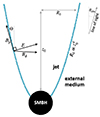 |
Fig. 1. Shape of the jet. The boundary radius, R0, is proportional to z0q, where z0 is the distance from the supermassive black hole. The value of the parameter q < 1 depends on the pressure profile of the external medium that collimates the jet. The line of sight makes an angle θobs with respect to the direction of the jet axis. |
We adopted a cylindrical coordinate system (R, ϕ, z), where  is directed along the jet axis. The electromagnetic fields can be presented as
 (1)
(1)
 (2)
(2)
where
 (3)
(3)
 (4)
(4)
The speed of light is set to c = 1. The angular velocity, Ω, and the poloidal magnetic field, Bp, are assumed to be independent of R. Numerical simulations show that this is a reasonable approximation (see, e.g., Fig. 4 of Komissarov et al. 2007).
The local jet opening angle, Θ, is determined by the shape of the magnetic flux surfaces. The boundary radius, R0, can be parametrized as ΩR0 = 31/4C(Ωz0)q, where C is a constant of order unity (Lyubarsky 2009). At the distance z0 from the black hole, one has Θ ≃ |Ez/ER|=qR/z0, which gives
 (5)
(5)
As we discuss in Appendix C, in the model of Lyubarsky (2009) the toroidal magnetic field is determined by
 (6)
(6)
Taking into account that ΩR0 ≫ 1 far beyond the light cylinder, from Eqs. (3) and (6) one can show that Bϕ ∼ ER ≫ Bp in the observer’s frame. However, the poloidal magnetic field cannot be neglected because the toroidal field and the electric field nearly cancel in the proper frame. The left panel of Fig. 2 shows the ratio of the toroidal and poloidal components of the magnetic field in the proper frame as a function of the distance from the jet axis. For small values of q (i.e., when the jet is nearly cylindrical) the poloidal component is larger than the toroidal component. For large q (i.e., when the jet opening angle increases) the toroidal component starts to dominate, especially near the jet boundary. As we explain in Sect. 3, these features are crucial for the polarization of the synchrotron radiation from the jet.
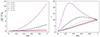 |
Fig. 2. Ratio of the toroidal and poloidal components of the magnetic field in the proper frame of the fluid (left panel) and bulk Lorentz factor of the fluid in the observer’s frame (right panel) as a function of the distance, R, from the jet axis. |
We assumed that the bulk velocity of the fluid, v, is equal to the drift velocity, which is
 (7)
(7)
The right panel of Fig. 2 shows the corresponding Lorentz factor, Γ = (1 − v2)−1/2 = (1 − E2/B2)−1/2. The value of ΩR0 is determined from the condition Γ(R0) = 10, which is the typical Lorentz factor of AGN jets. For small values of q, the Lorentz factor increases linearly with the radius (i.e., Γ ∼ ΩR). For large values of q, the Lorentz factor peaks at intermediate radii. One can show that near the jet boundary the Lorentz factor is determined by the curvature of the magnetic flux surfaces. Small and large values of q correspond respectively to the first and second collimation regimes identified by Lyubarsky (2009).
3. Polarization
In order to study the polarization of the synchrotron radiation from the jet, we assumed that the energy distribution of the emitting electrons in the proper frame is
 (8)
(8)
where Ke(R, z) is the proper electron number density. We also assumed that the distribution is isotropic.
The polarization of the synchrotron radiation from relativistic outflows has been investigated by several authors (e.g., Blandford & Königl 1979; Pariev et al. 2003; Lyutikov et al. 2003, 2005; Del Zanna et al. 2006). The Stokes parameters per unit length of a stationary jet are given by1
 (9)
(9)
 (10)
(10)
 (11)
(11)
where 𝒟 is the Doppler factor,  is the strength of the magnetic field component perpendicular to the line of sight, and χ is the angle between the polarization vector from a volume element and some reference direction in the plane of the sky that will be specified below. Primed quantities refer to the proper frame of the fluid. The integration volume is2 dV = R dR dϕ, where 0 < ϕ < 2π and 0 < R < R0. We also defined
 (12)
(12)
 (13)
(13)
where e and me are the charge and mass of the electron, ν is the observed radiation frequency, z is the cosmological redshift, D is the luminosity distance to the source, and ΓE is the Euler gamma function. The degree of linear polarization is
 (14)
(14)
and the EVPA, Ψ, of the synchrotron radiation from the entire emission region (assumed to be unresolved) is given by
 (15)
(15)
where 0 < Ψ < π.
Now we express the quantities that appear in Eqs. (9)–(11) as a function of the electromagnetic fields in the observer’s frame (our final expressions are given by Eqs. 21–23 below). We closely followed the framework developed by Del Zanna et al. (2006). The viewing angle θobs is measured with respect to the direction of the jet axis,  . Then, the unit vector directed toward the observer is
  . The polarization vector of the radiation from a volume element is (Lyutikov et al. 2003; Del Zanna et al. 2006)
 (16)
(16)
We took as a reference direction the projection of the jet axis on the plane of the sky, which is ![Mathematical equation: $ \hat{\mathbf{l}}=[( \hat{\mathbf{z}} \cdot \hat{\mathbf{n}})\hat{\mathbf{n}}-\hat{\mathbf{z}}]/\sqrt{1-(\hat{\mathbf{z}} \cdot \hat{\mathbf{n}})^2} $](/articles/aa/full_html/2024/10/aa50387-24/aa50387-24-eq22.gif) (note that
(note that  is the unit vector orthogonal to
  , and coplanar to
  and
and  ). Then, one has
  , and
, and  , or equivalently
 (17)
(17)
Since  ,
,  ,
,  are mutually orthogonal, any vector X can be conveniently decomposed as
  , where
  ,
,  ,
,  . Below we need the first and second components of
  , which are
 (18)
(18)
 (19)
(19)
and the third component of v = E × B/B2, which is
![Mathematical equation: $$ \begin{aligned} v_3 = \frac{\left[\left(B_z E_R-B_R E_z\right)\sin \phi -B_\phi E_z\cos \phi \right]\sin \theta _{\rm obs} + B_\phi E_R\cos \theta _{\rm obs}}{B^2}\cdot \end{aligned} $$](/articles/aa/full_html/2024/10/aa50387-24/aa50387-24-eq40.gif) (20)
(20)
Equation (17) gives  and
and  . Then one has
 (21)
(21)
The Doppler factor, ![Mathematical equation: $ \mathcal{D} =[\Gamma ( 1 - \mathbf{v} \cdot \hat{\mathbf{n}})]^{-1} $](/articles/aa/full_html/2024/10/aa50387-24/aa50387-24-eq44.gif) , can be presented as
, can be presented as
 (22)
(22)
Taking into account that v ⋅ B = 0, the strength of the magnetic field component perpendicular to the line of sight is (Del Zanna et al. 2006):  . As we demonstrate in Appendix D, this expression is equivalent to
 (23)
(23)
To calculate the Stokes parameters, one needs to specify the electron number density Ke. We considered two different scenarios: a constant number density, Ke = K0 (Sect. 3.1) and a constant magnetization, Ke ∝ B′2, where B′=B/Γ is the magnetic field strength in the proper frame (Sect. 3.2). We assumed that the viewing angle is θobs = 1/Γ(R0) = 0.1 rad. The effect of changing the viewing angle is discussed in Appendix A.
3.1. Constant number density
In the left panels of Fig. 3 we show the polarization degree Π and the EVPA obtained for a constant proper number density (i.e., Ke = K0) as a function of the power-law index, p, of the electron energy distribution. The spectrum of the emitted radiation is Fν ∝ ν−α, where α = (p − 1)/2. The typical value of the optical spectral index of HSP blazars is α ∼ 0.5 (Fossati et al. 1998; Abdo et al. 2011; Ghisellini et al. 2017), which is obtained for p = 2. The X-ray spectral index is typically within the range α ∼ 1.5–2.5, which is obtained for p = 4–6. Hereafter, we assume the optical and X-ray polarization to be respectively ΠO = Πp = 2 and Πp = 4 < ΠX < Πp = 6.
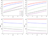 |
Fig. 3. Polarization degree, Π (top panels) and EVPA (bottom panels) as a function of the power-law index, p, of the electron energy distribution. When EVPA = 0 and EVPA = π/2, the EVPA is respectively parallel and perpendicular to the projection of the jet axis on the plane of the sky. In the left panels the proper number density is assumed to be constant, whereas in the right panels the magnetization is assumed to be constant. The viewing angle is assumed to be θobs = 0.1 rad. |
For small values of q, the polarization degree is close to the maximal one, which is Πmax = (p + 1)/(p + 7/3). For example, considering a jet with q = 0.2 we find3ΠX = 0.68–0.74 and ΠO = 0.58, whereas Πmax, X = 0.79–0.84 and Πmax, O = 0.69. The polarization degree is weakly chromatic, as ΠX/ΠO = 1.2. Considering q = 0.05–0.1, the polarization degree changes by less than a few percent with respect to the model with q = 0.2. The EVPA is nearly perpendicular to the projection of the jet axis on the plane of the sky, as expected since in the proper frame the magnetic field is predominantly poloidal (see Fig. 2).
For large values of q, the polarization degree is much smaller than Πmax. For q = 0.6 we find ΠX = 0.41–0.52 and ΠO = 0.25, and for q = 0.8 we find ΠX = 0.38–0.54 and ΠO = 0.20. The polarization degree is strongly chromatic, as ΠX/ΠO = 1.6–2.7. This effect is entirely due to the softening of the electron energy distribution at high energies (we assumed p = 2 for the optical emitting electrons, and p = 4–6 for the X-ray emitting electrons). The chromaticity is much stronger than for a uniform magnetic field, where the polarization degree is Πmax = (p + 1)/(p + 7/3) (Fig. 5 of Lyutikov et al. 2003 shows that the polarization degree can increase with p more rapidly than Πmax, consistent with our results). The EVPA is nearly parallel to the projection of the jet axis on the plane of the sky, as expected since in the proper frame the magnetic field is predominantly toroidal. For q ≳ 0.8 the polarization degree slightly increases, whereas the EVPA shows a continuous transition to EVPA = 0. As we discuss in Appendix B, an abrupt transition from EVPA = π/2 to EVPA = 0 is possible only for some special jet shapes.
3.2. Constant magnetization
In the right panels of Fig. 3 we show the polarization degree Π and the EVPA obtained for a constant magnetization (i.e., Ke ∝ B′2 = B2/Γ2). For small values of q, one has Bϕ2 − E2 ≪ Bp2 (see Fig. 2), and therefore B′2 = B2 − E2 ∼ Bp2. Since Bp is independent of R, the polarization degree and the EVPA are similar to the scenario with constant number density.
For large values of q, one has Bϕ2 − E2 ≫ Bp2, and therefore B′2 ∼ Bϕ2 − E2. Since Bϕ2 − E2 ∝ R4 (see Eq. 6), the proper number density has a sharp peak near the jet boundary. The polarization degree is smaller with respect to the scenario with a constant number density. For q = 0.6 we find ΠX = 0.40–0.51 and ΠO = 0.24, and for q = 0.8 we find ΠX = 0.15–0.26 and ΠO = 0.05. Larger values of q would give a lower polarization degree. For example, for q = 0.9 we find ΠX = 0.067–0.15 and ΠO = 0.016. In this case, the chromaticity is very strong, as ΠX/ΠO = 4.2–9.3. However, the peak bulk Lorentz factor would be very large.
4. Discussion
We studied the polarization of the synchrotron radiation from HSP blazars. We used the axisymmetric stationary model of Lyubarsky (2009) to calculate the jet electromagnetic fields, as appropriate for blazars in a quiescent state. In this model, the transverse size of the jet can be parameterized as R0 ∝ z0q, where z0 is the distance from the black hole. We considered two simple scenarios to populate the jet with nonthermal electrons (we assumed that either the magnetization or the electron proper number density across the jet is constant). The shape of the jet has a dramatic impact on the polarization:
-
For q ∼ 0.2 (a nearly cylindrical jet), the polarization degree is large and weakly chromatic (the X-ray and optical polarization degrees are respectively ΠX ∼ 70% and ΠO ∼ 60%). The EVPA is nearly perpendicular to the projection of the jet axis on the plane of the sky.
-
For q ∼ 0.6–0.8 (a nearly parabolic jet), the polarization degree is lower and becomes strongly chromatic. We find ΠX ∼ 15–50% and ΠO ∼ 5–25% (the ratio is typically ΠX/ΠO ∼ 2–5; however, the ratio can reach ΠX/ΠO ∼ 9 for q = 0.9). The EVPA is nearly parallel to the projection of the jet axis on the plane of the sky.
We emphasize that in our model the optical and X-ray emitting electrons are co-spatial and only differ in terms of the power-law index of their energy distributions. The chromaticity is due to the softening of the electron distribution at high energies and is much stronger than for a uniform magnetic field. The polarization degree and the EVPA are determined by the global structure of the electromagnetic fields within the jet (the effect of a random component of the fields is discussed below).
Our results are important for interpreting multifrequency polarimetric observations of HSP blazars (Liodakis et al. 2022; Di Gesu et al. 2022; Ehlert et al. 2023; Errando et al. 2024; Kim et al. 2024). The observed X-ray polarization degree is ΠX ∼ 10–20%, whereas the optical polarization degree is significantly smaller (ΠX/ΠO ∼ 2–7). The EVPA seems to align with the projection of the jet axis on the plane of the sky4. Our results show that the jet should be nearly parabolic (q ∼ 0.6–0.8), consistent with very long baseline interferometry observations of AGN jets on larger spatial scales (Mertens et al. 2016; Pushkarev et al. 2017; Kovalev et al. 2020; Boccardi et al. 2021).
Current multifrequency polarimetric observations of HSP blazars can hardly constrain the particle acceleration process. In our model the jet is Poynting-dominated, and therefore nonthermal particle acceleration is likely powered by magnetic reconnection rather than shocks (Sironi et al. 2015). The most energetic electrons trace the distribution of the reconnecting current sheets, as their cooling time is short. The Kelvin-Helmholtz instability at the interface between the jet and the external medium can produce current sheets near the jet boundary (Sironi et al. 2021). Instead, the kink instability can produce a more uniform distribution of current sheets across the jet (Alves et al. 2018; Davelaar et al. 2020). In the scenarios that we explored, the polarization degree and the EVPA are not very sensitive to the radial distribution of the electrons. As such, it is difficult to say whether reconnection is triggered by the Kelvin-Helmholtz or the kink instability.
We conclude by discussing some directions for future research:
(i) The electromagnetic fields may have a random component that changes on small spatial scales. If the random component is isotropic in the proper frame, and its strength is comparable to the regular component, the polarization degree decreases by a factor of ∼2, whereas the EVPA does not change (Granot & Königl 2003; Bandiera & Petruk 2016). A time-dependent random magnetic field can produce fluctuations of the polarization degree and EVPA (Marscher 2014).
(ii) Nonthermal electrons could be continuously accelerated at a certain distance from the black hole and then advected along the jet for a cooling length. Since the cooling length depends on the electron energy, this leads to “energy stratification,” as previously discussed for the shock acceleration scenario (Tavecchio et al. 2018, 2020). We emphasize that some energy stratification is expected in any conceivable scenario, as particles with a longer cooling time are advected farther away along the jet. The polarization degree is expected to decrease as the emission region becomes more spatially extended. This effect is chromatic (ΠO decreases more than ΠX because the corresponding electron cooling time is longer by a factor of  ).
).
(iii) Both optical and X-ray EVPA swings have now been observed (Marscher et al. 2008, 2010; Abdo et al. 2010; Larionov et al. 2013; Blinov et al. 2015, 2016, 2018; Kiehlmann et al. 2016; Di Gesu et al. 2023; Middei et al. 2023b). To explain the EVPA swings, one should abandon the axisymmetric stationary jet model that we used throughout this paper. The fact that optical and X-ray EVPA swings are not simultaneous suggests that, due to energy stratification, the emitting electrons are not exactly co-spatial (Di Gesu et al. 2023; Middei et al. 2023b).
Since we are dealing with ultra-relativistic particles, we neglected circular polarization and set V = 0.
The Stokes parameters per unit jet length provide good estimates of Π and EVPA when the emission region is not very extended. For example, taking dV = R dR dϕ dz, where z0 − Δz < z < z0, we find that Π and EVPA change by < 20% for Δz/z0 < 0.5. Our results do not depend on the exact location of the emission region (i.e., fixing Γ(R0) = 10 one finds that Π and EVPA are independent of z0).
The X-ray polarization degree depends on the power-law index of the electron energy distribution. ΠX = 0.68 and ΠX = 0.74 are obtained for p = 4 and p = 6, respectively.
The situation is far from clear, especially for the blazars 1ES 0229+200 (Ehlert et al. 2023) and Mrk 421 (Di Gesu et al. 2022). As noted in Di Gesu et al. (2022), the jet could bend by tens of degrees between the inner region (where the X-ray and optical emission are likely produced) and the outer region imaged in the radio band.
Acknowledgments
We are grateful to the anonymous referee for their constructive comments. We acknowledge insightful discussions with Rino Bandiera, Niccolò Bucciantini, Luca Del Zanna, and Jonathan Granot. We acknowledge financial support from the Marie Skłodowska-Curie Grant 101061217 (PI E. Sobacchi) and from a INAF Theory Grant 2022 (PI F. Tavecchio). This work has been funded by the European Union-Next Generation EU, PRIN 2022 RFF M4C21.1 (2022C9TNNX).
References
- Abdo, A. A., Ackermann, M., Ajello, M., et al. 2010, Nature, 463, 919 [NASA ADS] [CrossRef] [Google Scholar]
- Abdo, A. A., Ackermann, M., Ajello, M., et al. 2011, ApJ, 736, 131 [Google Scholar]
- Alves, E. P., Zrake, J., & Fiuza, F. 2018, Phys. Rev. Lett., 121, 245101 [NASA ADS] [CrossRef] [Google Scholar]
- Bandiera, R., & Petruk, O. 2016, MNRAS, 459, 178 [NASA ADS] [CrossRef] [Google Scholar]
- Blandford, R. D., & Königl, A. 1979, ApJ, 232, 34 [Google Scholar]
- Blandford, R. D., & Payne, D. G. 1982, MNRAS, 199, 883 [CrossRef] [Google Scholar]
- Blandford, R. D., & Znajek, R. L. 1977, MNRAS, 179, 433 [NASA ADS] [CrossRef] [Google Scholar]
- Blandford, R., Meier, D., & Readhead, A. 2019, ARA&A, 57, 467 [NASA ADS] [CrossRef] [Google Scholar]
- Blinov, D., Pavlidou, V., Papadakis, I., et al. 2015, MNRAS, 453, 1669 [NASA ADS] [CrossRef] [Google Scholar]
- Blinov, D., Pavlidou, V., Papadakis, I. E., et al. 2016, MNRAS, 457, 2252 [NASA ADS] [CrossRef] [Google Scholar]
- Blinov, D., Pavlidou, V., Papadakis, I., et al. 2018, MNRAS, 474, 1296 [CrossRef] [Google Scholar]
- Boccardi, B., Perucho, M., Casadio, C., et al. 2021, A&A, 647, A67 [NASA ADS] [CrossRef] [EDP Sciences] [Google Scholar]
- Böttcher, M. 2019, Galaxies, 7, 20 [Google Scholar]
- Davelaar, J., Philippov, A. A., Bromberg, O., & Singh, C. B. 2020, ApJ, 896, L31 [NASA ADS] [CrossRef] [Google Scholar]
- Del Zanna, L., Volpi, D., Amato, E., & Bucciantini, N. 2006, A&A, 453, 621 [NASA ADS] [CrossRef] [EDP Sciences] [Google Scholar]
- Di Gesu, L., Donnarumma, I., Tavecchio, F., et al. 2022, ApJ, 938, L7 [CrossRef] [Google Scholar]
- Di Gesu, L., Marshall, H. L., Ehlert, S. R., et al. 2023, Nat. Astron., 7, 1245 [NASA ADS] [CrossRef] [Google Scholar]
- Ehlert, S. R., Liodakis, I., Middei, R., et al. 2023, ApJ, 959, 61 [NASA ADS] [CrossRef] [Google Scholar]
- Errando, M., Liodakis, I., Marscher, A. P., et al. 2024, ApJ, 963, 5 [NASA ADS] [CrossRef] [Google Scholar]
- Fossati, G., Maraschi, L., Celotti, A., Comastri, A., & Ghisellini, G. 1998, MNRAS, 299, 433 [Google Scholar]
- Ghisellini, G., Righi, C., Costamante, L., & Tavecchio, F. 2017, MNRAS, 469, 255 [NASA ADS] [CrossRef] [Google Scholar]
- Granot, J., & Königl, A. 2003, ApJ, 594, L83 [NASA ADS] [CrossRef] [Google Scholar]
- Kiehlmann, S., Savolainen, T., Jorstad, S. G., et al. 2016, A&A, 590, A10 [NASA ADS] [CrossRef] [EDP Sciences] [Google Scholar]
- Kim, D. E., Di Gesu, L., Liodakis, I., et al. 2024, A&A, 681, A12 [NASA ADS] [CrossRef] [EDP Sciences] [Google Scholar]
- Komissarov, S. S., Barkov, M. V., Vlahakis, N., & Königl, A. 2007, MNRAS, 380, 51 [Google Scholar]
- Komissarov, S. S., Vlahakis, N., Königl, A., & Barkov, M. V. 2009, MNRAS, 394, 1182 [NASA ADS] [CrossRef] [Google Scholar]
- Kovalev, Y. Y., Pushkarev, A. B., Nokhrina, E. E., et al. 2020, MNRAS, 495, 3576 [NASA ADS] [CrossRef] [Google Scholar]
- Larionov, V. M., Jorstad, S. G., Marscher, A. P., et al. 2013, ApJ, 768, 40 [NASA ADS] [CrossRef] [Google Scholar]
- Liodakis, I., Marscher, A. P., Agudo, I., et al. 2022, Nature, 611, 677 [CrossRef] [Google Scholar]
- Lyubarsky, Y. 2009, ApJ, 698, 1570 [NASA ADS] [CrossRef] [Google Scholar]
- Lyubarsky, Y. 2010, MNRAS, 402, 353 [NASA ADS] [CrossRef] [Google Scholar]
- Lyubarsky, Y., et al. 2011, Phys. Rev. E, 83, 016302 [NASA ADS] [CrossRef] [Google Scholar]
- Lyutikov, M., Pariev, V. I., & Blandford, R. D. 2003, ApJ, 597, 998 [Google Scholar]
- Lyutikov, M., Pariev, V. I., & Gabuzda, D. C. 2005, MNRAS, 360, 869 [Google Scholar]
- Marscher, A. P. 2014, ApJ, 780, 87 [Google Scholar]
- Marscher, A. P., & Jorstad, S. G. 2021, Galaxies, 9, 27 [NASA ADS] [CrossRef] [Google Scholar]
- Marscher, A. P., Jorstad, S. G., D’Arcangelo, F. D., et al. 2008, Nature, 452, 966 [Google Scholar]
- Marscher, A. P., Jorstad, S. G., Larionov, V. M., et al. 2010, ApJ, 710, L126 [Google Scholar]
- Marshall, H. L., Liodakis, I., & Marscher, A. P. 2023, ArXiv e-prints [arXiv:2310.11510] [Google Scholar]
- Mertens, F., Lobanov, A. P., Walker, R. C., & Hardee, P. E. 2016, A&A, 595, A54 [NASA ADS] [CrossRef] [EDP Sciences] [Google Scholar]
- Middei, R., Liodakis, I., Perri, M., et al. 2023a, ApJ, 942, L10 [NASA ADS] [CrossRef] [Google Scholar]
- Middei, R., Perri, M., Puccetti, S., et al. 2023b, ApJ, 953, L28 [NASA ADS] [CrossRef] [Google Scholar]
- Pariev, V. I., Istomin, Y. N., & Beresnyak, A. R. 2003, A&A, 403, 805 [NASA ADS] [CrossRef] [EDP Sciences] [Google Scholar]
- Peirson, A. L., Negro, M., Liodakis, I., et al. 2023, ApJ, 948, L25 [NASA ADS] [CrossRef] [Google Scholar]
- Pushkarev, A. B., Kovalev, Y. Y., Lister, M. L., & Savolainen, T. 2017, MNRAS, 468, 4992 [Google Scholar]
- Romero, G. E., Boettcher, M., Markoff, S., & Tavecchio, F. 2017, Space Sci. Rev., 207, 5 [NASA ADS] [CrossRef] [Google Scholar]
- Sironi, L., Petropoulou, M., & Giannios, D. 2015, MNRAS, 450, 183 [Google Scholar]
- Sironi, L., Rowan, M. E., & Narayan, R. 2021, ApJ, 907, L44 [CrossRef] [Google Scholar]
- Tavecchio, F. 2021, Galaxies, 9, 37 [NASA ADS] [CrossRef] [Google Scholar]
- Tavecchio, F., Landoni, M., Sironi, L., & Coppi, P. 2018, MNRAS, 480, 2872 [NASA ADS] [CrossRef] [Google Scholar]
- Tavecchio, F., Landoni, M., Sironi, L., & Coppi, P. 2020, MNRAS, 498, 599 [NASA ADS] [CrossRef] [Google Scholar]
- Tchekhovskoy, A., McKinney, J. C., & Narayan, R. 2008, MNRAS, 388, 551 [NASA ADS] [CrossRef] [Google Scholar]
- Tchekhovskoy, A., McKinney, J. C., & Narayan, R. 2009, ApJ, 699, 1789 [NASA ADS] [CrossRef] [Google Scholar]
- Tchekhovskoy, A., Narayan, R., & McKinney, J. C. 2011, MNRAS, 418, L79 [NASA ADS] [CrossRef] [Google Scholar]
- Vlahakis, N. 2004, ApJ, 600, 324 [NASA ADS] [CrossRef] [Google Scholar]
Appendix A: Effect of the viewing angle
We investigated the dependence of the polarization degree on the viewing angle. We assumed that the proper number density of the emitting electrons is constant. In the top panel of Fig. A.1 we show the optical polarization degree, and in the bottom panel we show the X-ray polarization degree. Both ΠO and ΠX show a similar dependence on θobs. The most important difference is that ΠO is smaller than ΠX for a given θobs.
The polarization degree vanishes for θobs = 0, as expected from symmetry considerations. For q ∼ 0.2, the polarization degree rises almost abruptly to Πmax, and then decreases for large θobs. For q ∼ 0.5 − 0.8, the rise is more gradual, and the peak polarization is smaller than Πmax.
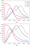 |
Fig. A.1. Optical polarization degree, ΠO = Πp = 2 (top panel) and X-ray polarization degree, ΠX = Πp = 4 (bottom panel) as a function of the viewing angle, θobs, which is expressed in radians. The proper number density of the emitting electrons is assumed to be constant. |
Appendix B: Special jet shapes
In the general case discussed in Sect. 3, the Stokes parameter U does not vanish. However, for the special jet shapes discussed below one finds U = 0. When U = 0, the EVPA can be either parallel or perpendicular to the projection of the jet axis on the plane of the sky.
Lyutikov et al. (2003) considered a conical jet with BR = Bz = 0. In this case, one has
 (B.1)
(B.1)
 (B.2)
(B.2)
 (B.3)
(B.3)
For a given viewing angle θobs, the Doppler factor is a function of R and cos ϕ:
 (B.4)
(B.4)
Since q12 + q22 is also a function of R and cos ϕ, one has
 (B.5)
(B.5)
Finally, one finds
 (B.6)
(B.6)
The functions f1, f2, f3 are defined through Eqs. (B.4)-(B.6). Substituting Eqs. (B.4)-(B.6) into Eq. (11), one finds
 (B.7)
(B.7)
where the function F can be expressed as a combination of f1, f2, f3. It is clear that U = 0 for any function F.
Pariev et al. (2003) and Lyutikov et al. (2005) considered a cylindrical jet with Ez = BR = 0. In this case, one has
 (B.8)
(B.8)
 (B.9)
(B.9)
 (B.10)
The Doppler factor is a function of R and sin ϕ:
 (B.11)
Since q12 + q22 is also a function of R and sin ϕ, one has
 (B.12)
Finally, one finds
 (B.13)
Substituting Eqs. (B.11)-(B.13) into Eq. (11), one finds
 (B.14)
which gives U = 0.
Appendix C: Details of the jet structure
When the jet is accelerated to bulk Lorentz factors Γ ≫ 1, Eq. (29) of Lyubarsky (2009) gives
 (C.1)
(C.1)
Following Lyubarsky (2009), we defined X = ΩR and Z = Ωz0. The shape of the flux surfaces was determined by their Eq. (74), which gives  , where Y = CZq. Substituting this expression into their Eq. (75), one finds
 (C.2)
(C.2)
Since the background magnetic field is assumed to be uniform, one has ψ/ψ0 = R2/R02 = X2/Ω2R02. As discussed above, one has also  . Then, one finds
 (C.3)
(C.3)
Eq. (6) immediately follows from Eqs. (C.1)-(C.3).
Appendix D: Perpendicular magnetic field
We calculated the strength of the magnetic field component perpendicular to the line of sight. First of all, we demonstrated two useful identities. The first identity is
![Mathematical equation: $$ \begin{aligned} \left[\left(\mathbf E \times \mathbf B \right)\cdot \hat{\mathbf{n }}\right]^2 = E^2B^2 - \left(\mathbf B \cdot \hat{\mathbf{n }} \right)^2 E^2 - \left(\mathbf E \cdot \hat{\mathbf{n }}\right)^2 B^2 \;, \end{aligned} $$](/articles/aa/full_html/2024/10/aa50387-24/aa50387-24-eq68.gif) (D.1)
(D.1)
which can be demonstrated as follows. Consider the vector  . One has
![Mathematical equation: $$ \begin{aligned} P^2 = \left(\mathbf E \times \mathbf B \right)^2 - \left[\left(\mathbf E \times \mathbf B \right)\cdot \hat{\mathbf{n }}\right]^2 = E^2B^2 - \left[\left(\mathbf E \times \mathbf B \right)\cdot \hat{\mathbf{n }}\right]^2 \;, \end{aligned} $$](/articles/aa/full_html/2024/10/aa50387-24/aa50387-24-eq70.gif) (D.2)
(D.2)
where we used the fact that E ⋅ B = 0. Since  , one also has
 (D.3)
(D.3)
Equation (D.1) immediately follows from Eqs. (D.2)-(D.3). The second identity, which is obtained using the first one, is
![Mathematical equation: $$ \begin{aligned} \frac{1}{\Gamma ^2\mathcal{D} ^2}&= \left[1-\frac{\left(\mathbf E \times \mathbf B \right)\cdot \hat{\mathbf{n }}}{B^2}\right]^2 = \nonumber \\&= 1-\frac{2 \left( \mathbf E \times \mathbf B \right)\cdot \hat{\mathbf{n }}}{B^2} + \frac{E^2}{B^2} -\frac{\left(\mathbf B \cdot \hat{\mathbf{n }} \right)^2 E^2}{B^4} -\frac{\left(\mathbf E \cdot \hat{\mathbf{n }}\right)^2}{B^2}. \end{aligned} $$](/articles/aa/full_html/2024/10/aa50387-24/aa50387-24-eq73.gif) (D.4)
(D.4)
The strength of the magnetic field component perpendicular to the line of sight is  . This equation can be presented as
 (D.5)
(D.5)
where we used Eq. (D.4) to obtain the final expression. Now consider the vector  . One has
 (D.6)
(D.6)
 (D.7)
(D.7)
From Eqs. (D.5)-(D.7), it follows that
 (D.8)
(D.8)
which is equivalent to Eq. (23).
All Figures
|
Fig. 1. Shape of the jet. The boundary radius, R0, is proportional to z0q, where z0 is the distance from the supermassive black hole. The value of the parameter q < 1 depends on the pressure profile of the external medium that collimates the jet. The line of sight makes an angle θobs with respect to the direction of the jet axis. |
| In the text | |
|
Fig. 2. Ratio of the toroidal and poloidal components of the magnetic field in the proper frame of the fluid (left panel) and bulk Lorentz factor of the fluid in the observer’s frame (right panel) as a function of the distance, R, from the jet axis. |
| In the text | |
|
Fig. 3. Polarization degree, Π (top panels) and EVPA (bottom panels) as a function of the power-law index, p, of the electron energy distribution. When EVPA = 0 and EVPA = π/2, the EVPA is respectively parallel and perpendicular to the projection of the jet axis on the plane of the sky. In the left panels the proper number density is assumed to be constant, whereas in the right panels the magnetization is assumed to be constant. The viewing angle is assumed to be θobs = 0.1 rad. |
| In the text | |
|
Fig. A.1. Optical polarization degree, ΠO = Πp = 2 (top panel) and X-ray polarization degree, ΠX = Πp = 4 (bottom panel) as a function of the viewing angle, θobs, which is expressed in radians. The proper number density of the emitting electrons is assumed to be constant. |
| In the text | |
Current usage metrics show cumulative count of Article Views (full-text article views including HTML views, PDF and ePub downloads, according to the available data) and Abstracts Views on Vision4Press platform.
Data correspond to usage on the plateform after 2015. The current usage metrics is available 48-96 hours after online publication and is updated daily on week days.
Initial download of the metrics may take a while.