| Issue |
A&A
Volume 681, January 2024
|
|
|---|---|---|
| Article Number | A57 | |
| Number of page(s) | 15 | |
| Section | The Sun and the Heliosphere | |
| DOI | https://doi.org/10.1051/0004-6361/202346928 | |
| Published online | 11 January 2024 | |
Helioseismic determination of the solar metal mass fraction⋆
1
Département d’Astronomie, Université de Genève, Chemin Pegasi 51, 1290 Versoix, Switzerland
e-mail: This email address is being protected from spambots. You need JavaScript enabled to view it.
2
STAR Institute, Université de Liège, Liège, Belgium
3
Sternberg Astronomical Institute, Lomonosov Moscow State University, 119234 Moscow, Russia
4
Theoretical Astrophysics, Department of Physics and Astronomy, Uppsala University, Box 516 751 20 Uppsala, Sweden
5
Centre Spatial de Liège, Université de Liège, Angleur-Liège, Belgium
Received:
17
May
2023
Accepted:
24
August
2023
Abstract
Context. The metal mass fraction of the Sun Z is a key constraint in solar modelling, but its value is still under debate. The standard solar chemical composition of the late 2000s has the ratio of metals to hydrogen as Z/X = 0.0181, and there was a small increase to 0.0187 in 2021, as inferred from 3D non-LTE spectroscopy. However, more recent work on a horizontally and temporally averaged ⟨3D⟩ model claim Z/X = 0.0225, which is consistent with the high values based on 1D LTE spectroscopy from 25 years ago.
Aims. We aim to determine a precise and robust value of the solar metal mass fraction from helioseismic inversions, thus providing independent constraints from spectroscopic methods.
Methods. We devised a detailed seismic reconstruction technique of the solar envelope, combining multiple inversions and equations of state in order to accurately and precisely determine the metal mass fraction value.
Results. We show that a low value of the solar metal mass fraction corresponding to Z/X = 0.0187 is favoured by helioseismic constraints and that a higher metal mass fraction corresponding to Z/X = 0.0225 is strongly rejected by helioseismic data.
Conclusions. We conclude that direct measurement of the metal mass fraction in the solar envelope favours a low metallicity, in line with the 3D non-LTE spectroscopic determination of 2021. A high metal mass fraction, as measured using a ⟨3D⟩ model in 2022, is disfavoured by helioseismology for all modern equations of state used to model the solar convective envelope.
Key words: Sun: helioseismology / Sun: oscillations / Sun: fundamental parameters / Sun: abundances
Full dataset is available at the CDS via anonymous ftp to cdsarc.cds.unistra.fr (130.79.128.5) or via https://cdsarc.cds.unistra.fr/viz-bin/cat/J/A+A/681/A57
© The Authors 2024
 Open Access article, published by EDP Sciences, under the terms of the Creative Commons Attribution License (https://creativecommons.org/licenses/by/4.0), which permits unrestricted use, distribution, and reproduction in any medium, provided the original work is properly cited.
This article is published in open access under the Subscribe to Open model. This email address is being protected from spambots. You need JavaScript enabled to view it. to support open access publication.
1. Introduction
The precise value of the solar metallicity has been an issue in solar modelling since the reappraisal of the carbon, nitrogen, and oxygen abundances in the 2000s (Allende Prieto et al. 2001, 2002; Asplund et al. 2004, 2006; Meléndez & Asplund 2008). The downwards revision of these and other elements reflects an improved understanding of the solar spectrum and is thanks to the development of 3D radiative-hydrodynamic simulations of the solar photosphere, as well as more complex model atoms for taking departures from local thermodynamic equilibrium (LTE) into account. These abundance revisions were summarised in Asplund et al. (2009, hereafter AGSS09). Further improvements have been made over the years (Scott et al. 2015b,a; Grevesse et al. 2015; Amarsi & Asplund 2017; Amarsi et al. 2018, 2021), culminating in a new solar abundance table that was presented in Asplund et al. (2021, hereafter AAG21), which results from the best 3D non-LTE analyses available for a very large number of elements. The authors found a metal mass fraction of Z = 0.0139, or Z/X = 0.0187 relative to hydrogen.
These abundance revisions have led to strong disagreements with classical helioseismic constraints, such as the position of the base of the convective envelope, the helium abundance in the convective envelope, and sound speed inversions, but also with neutrino fluxes (see Bahcall & Serenelli 2005; Basu & Antia 2008; Serenelli et al. 2009; Buldgen et al. 2019a; Christensen-Dalsgaard 2021, and refs therein). In an attempt to resolve these disagreements, several other spectroscopic analyses of the solar abundances have been presented in the literature over the years. In particular, a series of papers summarised in Caffau et al. (2011) determined a higher metallicity value than in AAG21, corresponding to Z/X = 0.0209. Many of the differences between the 2011 and previous abundance measurements were later attributed to the measurement of equivalent widths (e.g., Amarsi et al. 2019, 2020) rather than differences in the 3D models. More details, including of other works, can be found in AAG21.
More recently, Magg et al. (2022) carried out an analysis of the solar flux spectrum using a horizontally and temporally averaged 3D model (hereafter, ⟨3D⟩). They determined a high solar metallicity corresponding to Z/X = 0.0225. This is consistent with the 1D LTE value of Grevesse & Sauval (1998): Z/X = 0.0231. The authors reported having solved the so-called solar abundance problem by bringing back a high metallicity value.
There are several reasons to be sceptical of this claim. On the spectroscopic side, the analysis of Magg et al. (2022) is based on a ⟨3D⟩ model. The authors did not validate their model with respect to any solar constraints; previous attempts with other ⟨3D⟩ models illustrate they are vastly inferior to full 3D models (Uitenbroek & Criscuoli 2011; Pereira et al. 2013). Moreover, their results for their 18 neutral iron lines show a large range and standard deviation of 0.62 dex and 0.13 dex (compared to 0.10 dex and 0.03 dex, respectively, in AAG21), suggesting serious deficiencies in their analysis. We also note that their oxygen abundance of 8.77 dex, based on the blended 630 nm line and the 777 nm triplet that shows strong departures from LTE (Amarsi et al. 2016, 2018), is in disagreement with the values inferred from molecular OH lines (Amarsi et al. 2021). A more recent determination of the solar oxygen abundance from the same group (Pietrow et al. 2023) using the centre to limb spectra of one OI line puts the value at 8.73 dex, which is in closer agreement with AAG21, as well as other previous studies (Pereira et al. 2009; Amarsi et al. 2018).
On the solar modelling side, although the agreement with classical helioseismic constraints is improved with a high metallicity value, this is only the case when using classical standard solar models with outdated descriptions of the radiative opacities and macroscopic transport (see Buldgen et al. 2023, for a discussion). Numerous studies (see Christensen-Dalsgaard 2021, and references therein for a discussion) have pointed out that a degeneracy exists between abundances and opacities. As such, the agreement with most helioseismic constraints can just as well be restored through modifications to radiative opacities. Furthermore, taking into account macroscopic transport of chemicals due to the combined effects of rotation and magnetic instabilities could restore the agreement with the seismic helium value in the convective zone (Eggenberger et al. 2022). Indeed, none of the classical helioseismic constraints provide a direct measurement of the solar metallicity but rather indirect hints that solar calibrated models using a high metal mass fraction provide a better agreement (see e.g., Buldgen et al. 2023).
To resolve the debate, it may be necessary to measure the solar metallicity in a way that is independent from spectroscopy. This approach is linked to investigations of the properties of the solar convective envelope, and it has been attempted as early as the year 2000 (Baturin et al. 2000; Takata & Shibahashi 2001) by using the properties of the first adiabatic exponent,  , or the adimensional sound speed gradient,
  . Further studies were attempted in the early 2000s (Lin & Däppen 2005; Antia & Basu 2006; Lin et al. 2007), with varying results. These measurements are sensitive to the equation of state (EOS) of the solar plasma, and the most recent studies using modern EOSs have favoured a low metallicity value (Vorontsov et al. 2013, 2014; Buldgen et al. 2017). However, only rather low precision has been achieved so far, with inferred intervals ranging between [0.008,0.013]. Using an independent approach based on seismic calibration of solar standard models Houdek & Gough (2011) inferred a value of Z = 0.0142 ± 0.0005, in good agreement with (Asplund et al. 2021).
In this study, we improve, both in accuracy and precision, the methods used in Buldgen et al. (2017) to infer the chemical composition of the envelope. Our method is based on a combination of seismic reconstruction techniques from Buldgen et al. (2020) and recomputation of the thermodynamic conditions in the solar envelope using both FreeEOS and SAHA-S EOSs. From this detailed analysis, combined with linear inversions of the first adiabatic exponent, we are able to precisely infer the favoured metallicity value in the solar convective envelope. Our results are robust with respect to modifications of the EOS and also indicate that the SAHA-S EOS is favoured over FreeEOS.
2. Solar models
2.1. Evolutionary and seismic models
We started from a set of reference models computed with the Liège Stellar Evolution code (Scuflaire et al. 2008) using the physical ingredients listed in Table 1. The main properties of the models are summarised in Table 2. We also added the properties of model MB22-Phot, which is the reference standard solar model provided in Magg et al. (2022). Its envelope chemical composition, being the one advised, is used for comparisons with the inversion results in Sect. 4.2. These evolutionary models were computed using an extended calibration procedure similar to the model of Buldgen et al. (2023). All models in this work include macroscopic transport at the BCZ to reproduce the lithium depletion observed at the age of the Sun (Wang et al. 2021).
Physical ingredients of the solar models.
Envelope properties of the evolutionary solar models.
The extended calibration procedure uses four free parameters and four constraints. Namely, the mixing-length parameter, αMLT; the initial chemical composition (described using the initial hydrogen, X0, and metal mass fraction, Z0); and an adiabatic overshooting parameter, αOv, are the free parameters, and the solar radius, surface metallicity, solar luminosity, and the helioseismic position of the base of the convective envelope (r/R)BCZ are the constraints. This calibration procedure allowed us to have an excellent agreement not only on the radial position of the base of the convective envelope but also on the mass coordinate at the BCZ and the m75 constraint (namely, the mass coordinate at 0.75 R⊙) that Vorontsov et al. (2013) described as a key constraint to calibrate the value of entropy in the solar convective zone.
The models computed from these evolutionary sequences served as starting points for the construction of seismic models following Buldgen et al. (2020). These models show a much better agreement in the solar radiative envelope, intrinsically limiting the uncertainties coming from cross-term contributions in the last step of the envelope reconstruction procedure. Moreover, Buldgen et al. (2020) showed that their reconstruction approach significantly improved the agreement in entropy proxy plateau and the density profile in the convective envelope with respect to helioseismic constraints. Additionally, after the reconstruction by Buldgen et al. (2020), the m75 parameter was within 0.9822 ± 0.0002 determined from Vorontsov et al. (2013), which is essentially the density profile from a physical point of view and shows that our models would be of high quality, according to their criteria. Therefore, these models provide a robust starting point for detailed investigations of the properties of the solar envelope. The total set also provides adequate conditions for robustness tests on artificial data. More precisely, we used various EOSs to carry out the analysis, as this physical ingredient is the main source of potential inaccuracies in the models for our approach. As we focussed only on the solar envelope, the inversion is therefore unaffected by the choice of opacity tables used in the reference models. By construction, the calibrated evolutionary models have a different chemical composition in the convective envelope as a result of the physical ingredients (e.g., opacities or solar abundances; see e.g., Buldgen et al. 2019b for an illustration). However, through the seismic reconstruction procedure, this effect is erased (as shown in the right panel of Fig. 1), as the thermodynamical coordinates are then uniquely defined from the inversion and used as inputs for the scan in chemical composition.
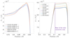 |
Fig. 1. Left panel: profile of Γ1 between the BCZ and 0.95 R⊙ for the solar models in Table 1. Right panel: entropy proxy profile, P/ρΓ1, as a function of normalised radius for the solar models of Table 1. The reference evolutionary models (‘Ref’) show a significant spread in entropy proxy plateau in the CZ that is corrected in the seismic models (‘Seismic’) by the seismic reconstruction procedure. |
As mentioned above, our main goal is to determine helioseismic constraints on the solar metal mass fraction and to compare them to spectroscopic abundance tables. Therefore, we compared our results to existing tables using acronyms defined as follows: GN93 is Grevesse & Noels (1993), GS98 is Grevesse & Sauval (1998), AGSS09 is Asplund et al. (2009), AAG21 is Asplund et al. (2021), and MB22 is Magg et al. (2022). In Table 2, models M1 and M2 were built using the recent abundances by Magg et al. (2022), whereas models A1, A2, and A3 were built using the Asplund et al. (2021) abundances.
We used two solar frequency datasets to assess the impact of the data on our results. The primary dataset (Dataset 1), used in Sects. 4.2 and 4.3, is the one used in Buldgen et al. (2020), which is a combination of the “optimal” dataset of Basu et al. (2009) combined with updated BiSON frequencies of Davies et al. (2014). The secondary dataset (Dataset 2) is a combination of BiSON data from Davies et al. (2014) and Basu et al. (2009) at low degree, but all modes with ℓ > 3 were taken from a 360-day asymmetric fitting from the MDI data of Larson & Schou (2015). The inversions were computed using the SOLA inversion technique (Pijpers & Thompson 1994), following prescriptions of Rabello-Soares et al. (1999) for trade-off parameter calibrations and using the InversionKit software in an adapted configuration.
2.2. Envelope properties
We first needed to investigate the details of the Γ1 profile, the entropy proxy profile, and the chemical composition in the envelope of the models. We started by plotting in the left panel of Fig. 1 the Γ1 profile of the evolutionary models and their respective entropy proxy profiles.
As shown in Fig. 1, the differences in the lower parts of the convective envelope are minute and strongly influenced by the EOS. However, it seems that a small trend still exists with metallicity. Namely, the higher the metallicity in the envelope, the lower the Γ1 value as a result of the higher signature of the ionisation of heavy elements in the case of a higher metal mass fraction. While of the order of 10−4, these differences may remain significant if the solar data is of high enough quality. These differences can be understood from the point of view of linear perturbations, as the relative differences in Γ1 may be written, assuming a given EOS, as
 (1)
(1)
where we have separated the relative differences in Γ1 in partial derivatives with respect to the various thermodynamical coordinates of the Γ1 function. As shown in Buldgen et al. (2017), the term linked with the Z derivatives has a broad maximum at around 0.75 R⊙, which is consistent with the analysis of Vorontsov et al. (2013, 2014). In practice, the inversion procedure relies on these signatures to determine the solar metallicity from a helioseismic point of view. As already mentioned in previous studies and as can be seen from Fig. 1, the inversion suffers from a dependency in the EOS. Therefore, the metal mass fraction inversion, just like the helium mass fraction inversion, is affected by the choice of the reference EOS.
In addition to EOS dependencies, it is worth noting that the other terms in Eq. (1) vary depending on the solar model considered. For example, the density and entropy proxy profiles in the envelope of solar evolutionary models strongly vary with the physical ingredients used in the calibration procedure. This is illustrated in Fig. 1 for high and low-metallicity solar models including macroscopic tran sport of chemicals and reproducing the lithium depletion observed in the Sun. These aspects must be taken into account by determining the actual density and pressure values in the solar convective zone from helioseismic data. Moreover, by using various models with transport prescriptions, we also used different helium mass fractions in the convective envelope in the inversion, therefore providing a robust analysis regarding the third term in Eq. (1).
3. Inversions of first adiabatic exponent
As shown in Fig. 1, the higher layers of the convective envelope around 0.95 R⊙ are strongly impacted by the EOS and helium ionisation. Disentangling the effects of the metal mass fraction in the solar envelope is extremely difficult. Therefore, we chose to divide the domain into two zones. Above 0.91 R⊙, we used the Γ1 profile to constrain the helium mass fraction, Y, whereas the lower part of the domain, below 0.91 R⊙, should not bear any strong signal of helium ionisation and should be more efficient in isolating the effects of the metallicity. We also observed that the slope of the Γ1 profiles between models computed with FreeEOS and those computed with SAHA-S are at odds around 0.87 R⊙. This plays an important role in the analysis of the solar data, as the final accepted Z value might be affected by the choice of the EOS. In what follows, we discuss our robust approach for determining Z while minimising such effects.
By looking at Γ1 inversions in the lower parts of the convective zone, we tried to determine very small corrections, namely, of the order of a few 10−4. These corrections are influenced by multiple effects: trade-off parameters of the inversions, surface effects, and cross-term contributions. Some can be tested but depend on the dataset used in the inversion procedure. Therefore, calibrating the overall procedure with artificial data is as important as carrying out the actual inversion using the observations. Moreover, a measure of the quality of the inversion can be made by verifying that the overall reconstruction of the seismic solar profile is consistent for various reference models. Should large model dependencies remain, the results would not necessarily be robust, and the trade-off parameters could be suboptimal.
3.1. The inversion strategy for metallicity determination
The determination of the metallicity was carried out using the dependencies of Γ1 on the chemical composition of the envelope. The first adiabatic exponent is a function of four thermodynamic coordinates, namely,
 (2)
(2)
Physically, the most interesting dependencies in the context of this study are those linked with the chemical composition. These result physically from the ionisations of helium and of the heavy elements at different temperatures in the solar envelope (see Baturin et al. 2022 for a discussion and illustrations). As shown in the left panel of Fig. 1 and explicitly visible in Eq. (1), an initial issue with helioseismic determinations of the solar metallicity is the dependency of the method on the EOS. The only solution to this problem is to actually test the method for various EOSs available to solar modellers. In our case, this was done by using the FreeEOS (Irwin 2012) and two versions of SAHA-S EOS (see also the SAHA-S web-site1Gryaznov et al. 2004, 2006, 2013; Baturin et al. 2013) in the modelling. The configuration used for FreeEOS is the recommended form reproducing the behaviour of the OPAL EOS (Rogers & Nayfonov 2002) and adopted in the latest generations of standard solar models (Vinyoles et al. 2017; Magg et al. 2022).
The other uncertainties regarding thermodynamic properties of the convective envelope were taken into account by using inversions for the density, the entropy proxy, and squared isothermal sound speed, u = P/ρ. These serve to determine the solar conditions as accurately as possible and act as sanity checks for the accuracy and precision of the overall method. To ensure maximal accuracy when working on actual solar data, we use the seismic models as the reference models for the final entropy, isothermal sound speed, and density inversions. The whole procedure for the metallicity inversion is summarised in Fig. 2. The first step is the extended solar calibration (blue box) that provides the initial conditions for the second step (orange box), the seismic reconstruction procedure of Buldgen et al. (2020), which damps the cross-term from the Ledoux discriminant in the variational equation and leads to an accurate depiction of solar thermodynamical conditions. The third step consists of inversions of density, using the (ρ, Γ1 kernels); squared isothermal sound speed (u = P/ρ), using the (u, Γ1 kernels); and Γ1, using the (A, Γ1 kernels) to determine the final thermodynamical coordinates (red box), which are then provided to the EOS routine.
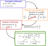 |
Fig. 2. Details of the fitting approach used to determine the chemical composition of the solar envelope. The four-step process is tailored to eliminate cross-term contributions at each step and maximise the accuracy, while the last step computed a reduced χ2 value for each subdomain (see main text). |
This process leads to the fourth step of the inference procedure (green box), during which a scan in X and Z is carried out using the seismic thermodynamical coordinates determined at the previous step in order to establish the optimal composition of the solar envelope. In this study, we considered X values within [0.70, 0.764] with a step of 0.001 and Z values within [0.01, 0.0176] with a step of 0.0004. Therefore a grid of 64 by 20 values was considered for X and Z when reconstructing the Γ1 profile. The normalised χ2 was computed using the Γ1 values from the last inversion, with N as the number of points; M as the number of free parameters, being two here (X and Z); and σ as the 1 σ uncertainty on the Γ1 from the inversion.
The domain of the solar convective envelope was separated into two zones. The first one, above T ≈ 9 × 10⁵ K, is dedicated to the determination of the metallicity. The second one, below T ≈ 5 × 10⁵ K, is dedicated to the determination of the hydrogen abundance. Due to the much higher abundance of helium in the solar envelope, the effects of the ionisation of helium and hydrogen largely dominate the properties of Γ1 at lower temperatures but not in the lower part of the CZ (for an illustration and a discussion, see Baturin et al. 2022).
4. Convective envelope composition
4.1. Artificial data
As a first test to determine the robustness of the method, we carried out a full analysis on artificial data. This was done by considering one of the seismic models as a reference model in the procedure while using an evolutionary model as the target. We considered three cases. In the first case (HH1), M1 plays the role of the target, and A2 is the reference. Thus, the effects of abundances and the EOS are both considered. In the second case (HH2), A1 is the target and A3 is the reference. In this case, no metallicity correction should be found, and the corrections are purely EOS effects. In the third case (HH3), M2 is the target and A2 is the reference. Only chemical composition effects are considered, as the EOS is the same for both models.
The dataset considered in the tests is exactly the same as the actual solar one, with the same uncertainties on individual modes. Therefore, the propagation of uncertainties; the calibration of the trade-off parameters; the effects of trade-offs and surface corrections, among others, should be as similar as possible with respect to the procedure used for actual solar data. We voluntarily chose high-Z models as targets to simulate the effect of a high-Z Sun, following the work of Magg et al. (2022), to see whether such as case could be recovered from the data.
Before entering in the details of the analysis of Fig. 3, we provide some additional details on the technicalities of the inversion. The full domain of the inversion spans from ≈0.72 R⊙ to ≈0.985 R⊙. Below this lowest value, the inversion might be significantly impacted by the effects of the boundary of the convective zone, as 0.72 can actually be considered quite low, and it would explain why a high trade-off parameter for the cross-term integral has been considered. Above 0.985, the inversion starts to be affected by the outer boundary conditions. The averaging kernels, despite showing good localisation, sometimes show sharp deviations. Moreover, the inversion is limited by the availability of other coordinates (namely  and ρ) that are more difficult to localise at such high radii with the considered dataset. Robustness with respect to surface effects and mass conservation constraint in the model might also play a role, and we chose to be conservative.
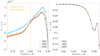 |
Fig. 3. Inversions of the Γ1 profile as a function of normalised radius for the artificial data (HH cases). Left panel: subdomain of the method for the Z determination (indicated by the orange vertical lines). Right panel: subdomain of the method for the X determination. |
The overall domain was then subdivided into two subdomains. The first one, at lower radii and higher temperatures, spans from ≈0.72 R⊙ to ≈0.85 R⊙. It counts about 17 points with Γ1 inversion values. Due to the higher temperatures, all H and He are ionised, and while both elements contribute to a large fraction of the electrons in these regions, the dips in Γ1 are mostly affected by the partial ionisation of metals. The effect is illustrated in Fig. 5 (upper panel) of Baturin et al. (2022), and one can see that the region of interest will mostly be influenced by oxygen and slightly influenced by carbon. Therefore, the Z inversion performed in this work mostly validates the abundance of oxygen, although the details of this should be confirmed from an analysis using the approach of Baturin et al. (2022). Due to the differences in Γ1 between FreeEOS and SAHA-S, between ≈0.85 R⊙ and ≈0.91 R⊙, we chose to initially neglect this region of the inversion (except in Sect. 4.3). While this might appear as a strong hypothesis, it is merely a choice of using 17 constraints in a region where all EOSs agree to determine one free parameter of the thermodynamical properties of the envelope, namely, Z. The underlying hypothesis of the method is that if FreeEOS and SAHA-S provide the same Γ1 values for the same coordinates, then the physics of the EOS must be robust2.
In this work, we focus on a global determination of Z. If the hypothesis that Z dominates largely in the properties of Γ1 in the first subdomain is valid, a scan in X and Z as discussed above should provide an almost horizontal valley of optimal values of Z for various values of X in an X − Zχ2 map. This is verified below.
The second subdomain is considered above ≈0.91 R⊙ up to ≈0.985 R⊙. We used it to constrain the X value in the convective envelope. This approach is similar to what has been done in the literature (e.g., Vorontsov et al. 1991; Basu & Antia 1995; Richard et al. 1998). The choice of going for X instead of Y does not affect the conclusions, as the couple X and Z determine a Y value, and in these low temperature regions, the effect of the metals is almost insignificant with respect to the uncertainties due to the EOS, surface effects, and inaccuracies in the thermodynamical coordinates. Again, this hypothesis can be checked when drawing the χ2 map, as the optimal solution should appear as a vertical valley in a X − Z plane. This is again verified below.
The results are illustrated in Fig. 3 for the Γ1 inversion. Comparing the full lines and the inversion results in the figure, we observed that the inversion reproduces the actual behaviour of the profile quite accurately. This means that the trade-off parameters have been well adjusted. When looking at all cases, we noted that in the left panel, the reconstructions have been able to grasp most of the features in the fitted areas. In each case where a high-Z model was a target (green and red symbols), the inversion managed to reproduce it quite nicely, while the discrepancies between FreeEOS and SAHA-S between ≈0.85 R⊙ and ≈0.91 R⊙ can be clearly seen for HH1. Similarly, when both models were of low-Z values but still exhibited significant differences due to their differing EOSs, the inversion managed to recover the proper range of metallicity. The same can be seen in the right panel of Fig. 3 for the helium ionisation zones.
The χ2 maps are illustrated in Fig. 4, with the left panel of each figure showing the results for the high-T subdomain used to determine Z and the right panel showing the results for the low-T subdomain used to determine X. We observed that the inversion actually provides a quite accurate estimate of both X and Z in all cases. While the Z inversion is not perfectlyhorizontal, a clear favoured region can be outlined, and using the information on X from the right panel to a favoured Z in the left panel helps further refine the information on Z. Here, we chose to limit the valley in X to the regions where the χ2 was below  , with
  being the lowest χ2 found for all values of X and Z used in the scan at low temperatures. This interval was then used to constrain the Z range in the valley, where the criterion is either to have χ2 < 1 whenever it is reached in an extended range or
  when the former criterion is not satisfied. In all cases this leads to a determined metallicity in agreement with the target value. We could see that this approach makes the technique less dependent on the details of the EOS at high temperatures. In practice, the change in reduced χ2 value induced by using the information of X (using the value of X with lowest χ2 to constrain Z) from the lower temperature is minimal and below one, meaning that the fit remains consistent. In all cases, this approach provides X and Z values that are in good agreement with the actual values of the models. For HH1, the X interval found is [0.724, 0.733] and the Z interval is [0.0160, 0.0170], with the solution being X = 0.732, Z = 0.01647. For HH2, the X interval found is [0.734, 0.738], and the Z interval is [0.0136, 0.0142], with the solution being X = 0.7386, Z = 0.01374. Finally, for HH3, the X interval found is [0.727, 0.729], and the Z interval is [0.0163, 0.0169], with the solution being X = 0.73056, Z = 0.01644. While slight biases can be observed for X, a clear result is that a low-Z Sun cannot be mistaken for a high-Z Sun using the current modern EOSs and that the provided interval predicts the correct value. Actual reduced χ2 differences between the high-Z and low-Z models range between a factor of five and eight for the scan in metallicity. The high χ2 values for the X inversion are found in the cases for which the EOS is different between the target and the reference models. In these cases, the χ2 values keep values of about 1000 or a few hundred at best. This is due to large discrepancies between the EOSs, amplified by the very small uncertainties of the SOLA inversion in regions where the method might actually be less robust (for reasons mentioned above). The colour scale in Fig. 4 is as follows: For the high-T subdomain used to determine Z; white corresponds to χ2 < 1, successive shades of blue to χ2 < 3, χ2 < 5, and χ2 < 6; and yellow corresponds to χ2 > 15. For the low-T subdomain used to determine X, white corresponds to
  ; successive shades of blue to
  ,
,  , and
, and  ; and yellow corresponds to
  , with
  for HH1, 419 for HH2, and 22 for HH3.
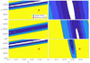 |
Fig. 4. Resulting χ2 map of the X and Z scan for the artificial data (HH exercises). The green and red crosses indicate the target and reference model, respectively. The upper panels are for HH1, middle panels are for HH2, and the lower panels are for HH3. The left panels are associated with the high-T subdomain for the Z determination, while the right panels are associated with the low-T subdomain used to determine X. |
4.2. Solar data
We start this section by presenting the Γ1 inversion results in Fig. 5 for each of the five seismic models presented in Sect. 2. It appears that the inversions plotted using the symbols of various colours are consistent with each other for all models. This gives confidence that the Γ1 profile has been accurately determined in a model-independent way.
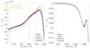 |
Fig. 5. Inversions of the Γ1 profile as a function of normalised radius determined from actual solar data. Left panel: subdomain of the method for the Z determination (indicated by the vertical orange lines). Right panel: subdomain of the method for the X determination. The orange curves are associated with reconstructions using FreeEOS, the purple curves are associated with reconstructions using SAHA-S, and the blue and red curves are associated with models M1 and M2 and A1 and A2, respectively. |
A quick look at the left panel of Fig. 5 shows that the Magg et al. (2022) models, denoted by the blue dashed lines, are already at odds with the data in the lower part of the convective zone, while this is not the case, or at least less the case, of the AAG21 models shown in red. A second observation on the slope of Γ1 between 0.85 R⊙ and 0.91 R⊙ indicated that solar data seems to strongly favour the SAHA-S EOS. However a physical explanation for these differences remains to be provided, as it could have multiple origins (e.g., coulomb correction, abundance of specific individual elements Trampedach et al. 2006). This observation confirms that the metallicity can be inferred most robustly between 0.72 and 0.85 R⊙. As mentioned in the previous section, we thus have 17 Γ1 inversion values for the first subdomain. Tests with the full profile between 0.72 and 0.91 R⊙ were also performed and are reported in Sect. 4.3.
In the left panel of Fig. 5, the best-fit profiles using FreeEOS between 0.72 and 0.85 R⊙ are indicated by the orange curves, while those using SAHA-S EOS are shown by the dark blue curves. These models also reproduce the solar data up to 0.91 R⊙ very well. However, these additional points are not included in the fit yet. For each EOS, the curves obtained through the reconstruction are essentially the same, meaning that the procedure is independent of the reference model and that only the assumed EOS might affect the final result. This effect is however mitigated by limiting the first subdomain between 0.72 and 0.85 R⊙.
The right panel of Fig. 5 shows the helium second ionisation zone. In this case, the situation is reversed, as the Magg et al. (2022) models, with their higher helium abundance in the solar convective zone, are in much better agreement than the AAG21 models. This was confirmed using the Γ1 reconstruction that favours very high helium abundances in the solar convective envelope. Again, all inversion points tend to agree with each other, providing confidence in the robustness of the approach. However, the points above 0.98 R⊙ might be influenced by boundary effects, surface effects, or slight inaccuracies in the determination of the ρ and u coordinates, as OLA inversions tend to be less accurate at the borders of the domain (Backus & Gilbert 1968; Pijpers & Thompson 1994).
Nevertheless, the results can be used to compute an χ2 map for the two subdomains, that is, between 0.72 and 0.85 R⊙ to constrain Z, and between 0.91 and 0.985 R⊙ to constrain X. Combining the optimal X and Z found in both subdomains, we obtained an accurate estimate of both parameters, as demonstrated on artificial data in the previous section.
The results are illustrated in Figs. 6 and 7, where the χ2 maps show that the assumption of separating the domain works quite well. Indeed, the optimal solution in the right panels are almost vertical, indicating that there is little dependence on the metallicity and that, as expected, X dominates the solution (due to its direct impact on Y and thus on the reproduction of the properties of the helium ionisation regions). Similarly, at high temperatures, a clear region in Z is outlined as the optimal solution. It is also clear that the higher temperature layers bear little to no information on X, as the material is clearly fully ionised. Thus, there is no clear trace left in the Γ1 profile to directly infer X. Therefore, as already seen in the HH exercise, one can use the information on X from lower temperatures to constrain the optimal interval for Z in the observed χ2 valley in the left panels of Figs. 6 and 7. This provides, independently of the EOS used (but assuming that either FreeEOS or SAHA-S is equally good in representing the plasma in the solar envelope), a final X interval between [0.715, 0.730] and a final Z interval between [0.0132, 0.0148] for the first dataset studied here.
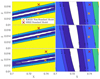 |
Fig. 6. Resulting χ2 map of the X and Z scan for solar data using model A2 (upper panels), A3 (middle panel), and M2 (lower panels) in the procedure and using either SAHA-S v7 or SAHA-S v3. The orange and red crosses indicate the positions of the AAG21 model including rotation and magnetic fields and the MB22 standard solar model, respectively (values from their paper). The left panel is associated with the high-T subdomain for the Z determination, while the right panel is associated with the low-T subdomain used to determine X. |
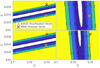 |
Fig. 7. Same as Fig. 6 for models A1 (upper panels) and M1 (lower panels), using FreeEOS in the reconstruction. The left panel is associated with the high-T subdomain for the Z determination, while the right panel is associated with the low-T subdomain used to determine X. |
Using SAHA-S (v3 or v7) in the analysis, the colour scale in Fig. 6 is as follows: For the high-T subdomain, white corresponds to χ2 < 1; successive shades of blue to χ2 < 3, χ2 < 5, and χ2 < 6; and yellow corresponds to χ2 > 15. For the low-T subdomain used to determine X, white corresponds to  ; successive shades of blue to
  ,
,  , and
, and  ; and yellow corresponds to
  , where
  for model A2, 3229 for model A3, and 2855 for model M2.
The colour scale in Fig. 7, where FreeEOS was used in the analysis, is as follows: For the high-T subdomain, white corresponds to  ; successive shades of blue to
  ,
,  , and
, and  ; and yellow corresponds to
  , where
  starting from model A1 and 3.14 starting from model M1. For the low-T subdomain used to determine X, white corresponds to
  ; successive shades of blue to
  ,
,  , and
, and  ; and yellow corresponds to
  , where
  starting from model A1 and 1236 starting from model M1. The explanation for the χ2 values always being greater than one in the high-T domain is due to the use of FreeEOS. This means that, overall, SAHA-S tends to provide better fits to solar data than FreeEOS at higher temperatures. However, FreeEOS tends to provide a better fit for the low-T domain overall, although none of the χ2 values match as well as in HH3, suggesting inaccuracies in the EOS in these low-T regimes and perhaps systematics in the inversion.
4.3. Assuming the equation of state known
As mentioned above, SAHA-S EOS provides a much better agreement with solar data than FreeEOS. Therefore, we found it is worth investigating what conclusions we can draw using the full set of Γ1 points and assuming SAHA-S as the EOS describing the solar material. We checked whether in these conditions one may infer individual element abundances, as carried out in Baturin et al. (2022). To do so, we attempted to reconstruct Γ1 using either the AGSS09 or the MB22 abundances, with X and Z as free parameters, starting from both model M1 and A2.
The results are illustrated in Fig. 8 for the Γ1 profiles. One can see that a small difference can be made between individual ratios of elements of AGSS09 and MB22, though not at a high level of significance. However, a low-Z value is still strongly favoured in the χ2 map illustrated in Fig. 9. In both cases, a Z value in line with AAG21 is favoured, while the low-Z valley seems to be a bit wider if individual ratios of elements of AGSS09 are assumed. This implies that while the Γ1 profile favours a low-Z value, in line with the AAG21 photospheric abundances, it might be difficult to disentangle the contribution of individual elements, although trying to pick some dominant trends regarding oxygen would still be worth attempting.
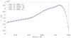 |
Fig. 8. Inversions of the Γ1 profile as a function of normalised radius determined from solar data assuming SAHA-S v7 as the EOS and changing the ratios of individual elements in the table (from MB22 to AAG21). Two reference models were used in the procedure: models M1 and A2. The results of the reconstructions are plotted in various colours. The red curve overplots the light blue one, and the purple curve overplots the green one. Each symbol depicts the Γ1 inversion results for the associated model (M1 or A2). |
The colour scale in Fig. 9, where SAHA-S was used in the analysis, is as follows. White corresponds to  . Successive shades of blue correspond to
  ,
,  , and
, and  . Yellow corresponds to
  . Starting from model A2 and the AAG21 abundances (upper-right panel),
  ; for model A2 with either MB22 (upper-left panel)
  ; and starting from model M1 with the MB22 (lower-right panel) and AAG21 abundances (lower-left panel)
  and 4.2, respectively.
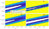 |
Fig. 9. Resulting χ2 map of the X and Z scan for the solar data fitting of Γ1 between 0.72 R⊙ and 0.91 R⊙. The orange crosses indicate the positions of the AAG21 model including rotation and magnetic fields, and the red crosses indicate the MB22 standard solar model (MB22-Phot in Table 2). Values are from their paper. The upper panels used the A2 model, and the lower panels used the M1 model. The left panels used MB22 individual elements, and the right panels used AAG21 individual elements. |
4.4. Impact of the dataset
We performed a final test using more recent MDI data from Larson & Schou (2015) in order to determine whether the trends picked in the previous sections are spurious or not. For this test, the whole calibration procedure was carried out again from the start. The results of the Γ1 inversions for models M1 and A2 are illustrated in Fig. 10. Again, a clear rejection of the high-Z solution of Magg et al. (2022) can be observed in the left panel of Fig. 10.
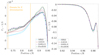 |
Fig. 10. Inversions of the Γ1 profile as a function of normalised radius in the solar enveloped, determined using the Larson & Schou (2015) dataset. Left panel: subdomain of the method for the Z determination (indicated by the orange vertical lines). Right panel: subdomain of the method for the X determination. The green curve and symbols are associated with model M1 (FreeEOS), whereas the purple curve and symbols are associated with model A2 (SAHA-S v7). The red and blue lines illustrate models A1 and A2 and M1 and M2, respectively. |
In this case, the reconstruction procedure struggled a bit more to reproduce the Γ1 values in the lower part of the convective envelope. SAHA-S EOS is still favoured between 0.85 R⊙ and 0.91 R⊙, but even the SAHA-S models struggled to reconstruct the profile. Nevertheless, as shown by the blue and red curves, low-Z models (in red) are strongly favoured over high-Z models (in blue) for the lower part of the CZ (left panel), while a high Y value is still favoured (right panel). The effects were confirmed for both test cases using model M1 and model A2.
The χ2 maps illustrated in Fig. 11 further confirm these trends, with low-Z values being strongly favoured over high-Z values. However, in this case, a slightly lower value of Z seems to be favoured. This might be similar to the trend seen in Vorontsov et al. (2013, 2014). We did however see that this time, the valley in X is almost perfectly vertical, with a slightly higher Y interval than in the previous sections. The overall fit in Z is somewhat more difficult given the strong deviations in the first few points in the deep convective zone (around 0.75 R⊙). In this case again, a factor between six and ten is found between the optimal solution at low Z and the MB22 standard solar model. While the AAG21 non-standard model performs better, it is still unable to reach the low X regime favoured by the inversion.
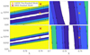 |
Fig. 11. Resulting χ2 map of the X and Z scan for solar data (Larson & Schou 2015) using model A2 in the procedure and fitting Γ1 between 0.72 R⊙ and 0.85 R⊙. The orange and red crosses indicate the positions of the AAG21 model including rotation and magnetic fields and the MB22 standard solar model, respectively (values from their paper). |
The colour scale in Fig. 11, using SAHA-S in the analysis, is as follows: For the high-T subdomain, white corresponds to  ; successive shades of blue to
  ,
,  ; and yellow corresponds to
  , with
  starting from model A2 using SAHA-S v7 and
  starting from model M1 and using FreeEOS. For the low-T subdomain used to determine X, white corresponds to
  ; successive shades of blue to
  ,
,  , and
, and  , and yellow corresponds to
  , with
  , starting from model A2 and using SAHA-S v7 and
  starting from model M1 and using FreeEOS. The trend we observed here is the opposite of what was seen before, with SAHA-S being favoured at low T, while FreeEOS is favoured between 0.72 and 0.85 R⊙.
4.5. Summary
To provide a global view of the inversion results, we had to combine the information of the χ2 for both datasets and all test cases. This was done and is shown in Fig. 12 and in Table 3. In the table, each line represents a full inversion procedure, from the determination of the seismic model to the reconstruction of the Γ1 profile to the chemical composition determinations. Some cases, in line 5 and 6, are those for which a different EOS than that of the reference model was used in the Γ1 reconstruction procedure. We chose to use the limits of the white areas in the χ2 maps of the hydrogen determinations to derive confidence intervals that would be used to extract the associated metallicity intervals. As shown in Sect. 4.1, this allowed us to accurately recover the actual values in the exercises with artificial data.
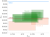 |
Fig. 12. Summary of the inversion procedure for the various models, datasets, and EOSs. The green and red rectangles represent the intervals provided from the analysis of Sects. 4.2 and 4.4, respectively. The blue and red lines indicate the solar metallicity value from Magg et al. (2022; MB22) and Asplund et al. (2021; AAG21), respectively. |
Summary of the inversion results for various EOSs and datasets.
We note that the size of the rectangles depends on other parameters, such as dataset and EOS, as these will change the landscape of the χ2. Our approach shows that the metallicity interval determined from a detailed helioseismic analysis of the properties of the solar envelope strongly favours the Asplund et al. (2021) abundances over the Magg et al. (2022) abundances.
5. Conclusion
The conclusions of this study are straightforward: The inversions of the solar data used to determine the Γ1 profile in the solar convective envelope do not favour the revision of the abundances of Magg et al. (2022) back to the old Grevesse & Sauval (1998) metallicity value. As seen from Fig. 12, this independent measurement of the solar metallicity from seismic analyses of the solar envelope strongly favours AAG21, as well as a high Y value in the convective envelope. The situation for the Magg et al. (2022) abundances is actually worse because the strongest rejection is found for a high-Z, high-Y model, which corresponds to the output of an MB22 model reproducing the solar luminosity. The situation worsens further for MB22 models including macroscopic transport to reproduce the lithium depletion at the age of the Sun (Buldgen et al. 2023).
Regarding helium, it also appears that the high Y value favoured here cannot be attained solely by including the effects of macroscopic transport in low-Z models. A revision of nuclear reaction rates or opacities at high T is required to reconcile solar models with the analysis performed here (Ayukov & Baturin 2017).
The method implemented here has a few caveats. For instance, the inversion is quite difficult, as trade-off parameters have to be adjusted for each dataset, and artificial data plays a key role in the calibration. Therefore, the results cannot be obtained on a large scale with numerous datasets. Based on supplementary investigations, suboptimal trade-off parameters do not change the conclusions but rather push towards lower Z values. Testing on more datasets might be done incrementally in the future, but it seems unlikely to change the conclusions. Future revisions of the EOS or the availability of new tables would be interesting for testing the physical effects in the EOS and could further confirm our results3.
An additional limitation of the method is the treatment of surface effects, chosen here to be dealt with using a sixth order polynomial form, as in Rabello-Soares et al. (1999). Experiments with both artificial data and changes to the order of the polynomial correction have been conducted to ensure robustness, but pushing towards higher degrees might need more detailed functional forms (Di Mauro et al. 2002), and the robustness and precision of the method would be further improved by using a more accurate modelling approach of the surface layers (Spada et al. 2018; Jørgensen et al. 2021). Further investigations on the systematics of such inversions are therefore required to further pin down the chemical composition of the solar envelope as are detailed comparisons of the available EOSs of the solar material.
Nevertheless, from our detailed helioseismic analysis of the solar envelope using an advanced seismic inversion approach and up-to-date EOSs of the latest generation of solar models, we conclude that the solar metallicity in the convective envelope lies in the range of 0.0120 − 0.0151, and the solar hydrogen mass fraction in the envelope lies in 0.715 − 0.730, resulting in a (Z/X)⊙ value between 0.0168 and 0.0205. Moreover, high-metallicity models using the Magg et al. (2022), Grevesse & Sauval (1998), or Grevesse & Noels (1993) abundances are rejected, as a steep slope in χ2 values was observed in all cases, with the χ2 values of high-metallicity solar envelope models being a factor of 6–20 times higher than those of low-metallicity models, independent of the EOS used and for two different helioseismic datasets. This independent measurement of the solar metallicity therefore strongly supports the AAG21 abundances (Asplund et al. 2021) over the MB22 abundances (Magg et al. 2022), in line with previous studies using modern EOSs (Vorontsov et al. 2013, 2014; Buldgen et al. 2017). Compared to the previous studies, our method provides a much more robust and precise inference, exploiting the properties of existing EOSs of the solar material.
We mention that the observed discrepancies between 0.85 R⊙ and 0.91 R⊙ do not influence the conclusions of the study on solar data. Rather, it makes the procedure more difficult regarding FreeEOS in the actual solar data analysis, but this does not affect the conclusion that if the Sun was high-Z, we should pick up the signal in the Γ1 profile.
For example, the latest revision of the MHD EOS (Trampedach priv. comm.).
Acknowledgments
The authors thank the referee for their careful reading of the manuscript. G.B. is funded by the SNF AMBIZIONE grant No 185805 (Seismic inversions and modelling of transport processes in stars). A.M.A. gratefully acknowledges support from the Swedish Research Council (VR 2020-03940). We acknowledge support by the ISSI team “Probing the core of the Sun and the stars” (ID 423) led by Thierry Appourchaux. The authors thank J. Christensen-Dalsgaard and S. Vorontsov for the detailed reading of the manuscript and the numerous suggestions.
References
- Allende Prieto, C., Lambert, D. L., & Asplund, M. 2001, ApJ, 556, L63 [Google Scholar]
- Allende Prieto, C., Lambert, D. L., & Asplund, M. 2002, ApJ, 573, L137 [NASA ADS] [CrossRef] [Google Scholar]
- Amarsi, A. M., & Asplund, M. 2017, MNRAS, 464, 264 [Google Scholar]
- Amarsi, A. M., Asplund, M., Collet, R., & Leenaarts, J. 2016, MNRAS, 455, 3735 [NASA ADS] [CrossRef] [Google Scholar]
- Amarsi, A. M., Barklem, P. S., Asplund, M., Collet, R., & Zatsarinny, O. 2018, A&A, 616, A89 [NASA ADS] [CrossRef] [EDP Sciences] [Google Scholar]
- Amarsi, A. M., Barklem, P. S., Collet, R., Grevesse, N., & Asplund, M. 2019, A&A, 624, A111 [NASA ADS] [CrossRef] [EDP Sciences] [Google Scholar]
- Amarsi, A. M., Grevesse, N., Grumer, J., et al. 2020, A&A, 636, A120 [NASA ADS] [CrossRef] [EDP Sciences] [Google Scholar]
- Amarsi, A. M., Grevesse, N., Asplund, M., & Collet, R. 2021, A&A, 656, A113 [NASA ADS] [CrossRef] [EDP Sciences] [Google Scholar]
- Antia, H. M., & Basu, S. 2006, ApJ, 644, 1292 [NASA ADS] [CrossRef] [Google Scholar]
- Asplund, M., Grevesse, N., Sauval, A. J., Allende Prieto, C., & Kiselman, D. 2004, A&A, 417, 751 [NASA ADS] [CrossRef] [EDP Sciences] [Google Scholar]
- Asplund, M., Grevesse, N., & Jacques Sauval, A. 2006, Nucl. Phys. A, 777, 1 [CrossRef] [Google Scholar]
- Asplund, M., Grevesse, N., Sauval, A. J., & Scott, P. 2009, ARA&A, 47, 481 [NASA ADS] [CrossRef] [Google Scholar]
- Asplund, M., Amarsi, A. M., & Grevesse, N. 2021, A&A, 653, A141 [NASA ADS] [CrossRef] [EDP Sciences] [Google Scholar]
- Ayukov, S. V., & Baturin, V. A. 2017, Astron. Rep., 61, 901 [NASA ADS] [CrossRef] [Google Scholar]
- Backus, G., & Gilbert, F. 1968, Geophys. J., 16, 169 [NASA ADS] [CrossRef] [Google Scholar]
- Bahcall, J. N., & Serenelli, A. M. 2005, ApJ, 626, 530 [NASA ADS] [CrossRef] [Google Scholar]
- Basu, S., & Antia, H. M. 1995, MNRAS, 276, 1402 [NASA ADS] [Google Scholar]
- Basu, S., & Antia, H. M. 2008, Phys. Rep., 457, 217 [Google Scholar]
- Basu, S., Chaplin, W. J., Elsworth, Y., New, R., & Serenelli, A. M. 2009, ApJ, 699, 1403 [NASA ADS] [CrossRef] [Google Scholar]
- Baturin, V. A., Däppen, W., Gough, D. O., & Vorontsov, S. V. 2000, MNRAS, 316, 71 [NASA ADS] [CrossRef] [Google Scholar]
- Baturin, V. A., Ayukov, S. V., Gryaznov, V. K., et al. 2013, in Progress in Physics of the Sun and Stars: A New Era in Helio- and Asteroseismology, eds. H. Shibahashi, & A. E. Lynas-Gray, ASP Conf. Ser., 479, 11 [Google Scholar]
- Buldgen, G., Salmon, S. J. A. J., Noels, A., et al. 2017, MNRAS, 472, 751 [NASA ADS] [CrossRef] [Google Scholar]
- Buldgen, G., Salmon, S., & Noels, A. 2019a, Front. Astron. Space Sci., 6, 42 [NASA ADS] [CrossRef] [Google Scholar]
- Buldgen, G., Salmon, S. J. A. J., Noels, A., et al. 2019b, A&A, 621, A33 [NASA ADS] [CrossRef] [EDP Sciences] [Google Scholar]
- Buldgen, G., Eggenberger, P., Baturin, V. A., et al. 2020, A&A, 642, A36 [EDP Sciences] [Google Scholar]
- Baturin, V. A., Oreshina, A. V., Däppen, W., et al. 2022, A&A, 660, A125 [NASA ADS] [CrossRef] [EDP Sciences] [Google Scholar]
- Buldgen, G., Eggenberger, P., Noels, A., et al. 2023, A&A, 669, L9 [NASA ADS] [CrossRef] [EDP Sciences] [Google Scholar]
- Caffau, E., Ludwig, H. G., Steffen, M., Freytag, B., & Bonifacio, P. 2011, Sol. Phys., 268, 255 [Google Scholar]
- Christensen-Dalsgaard, J. 2021, Liv. Rev. Sol. Phys., 18, 2 [NASA ADS] [CrossRef] [Google Scholar]
- Davies, G. R., Broomhall, A. M., Chaplin, W. J., Elsworth, Y., & Hale, S. J. 2014, MNRAS, 439, 2025 [Google Scholar]
- Di Mauro, M. P., Christensen-Dalsgaard, J., Rabello-Soares, M. C., & Basu, S. 2002, A&A, 384, 666 [NASA ADS] [CrossRef] [EDP Sciences] [Google Scholar]
- Eggenberger, P., Buldgen, G., Salmon, S. J. A. J., et al. 2022, Nat. Astron., 6, 788 [NASA ADS] [CrossRef] [Google Scholar]
- Grevesse, N., & Noels, A. 1993, in Origin and Evolution of the Elements, eds. N. Prantzos, E. Vangioni-Flam, & M. Casse, 15 [Google Scholar]
- Grevesse, N., & Sauval, A. J. 1998, Space Sci. Rev., 85, 161 [Google Scholar]
- Grevesse, N., Scott, P., Asplund, M., & Sauval, A. J. 2015, A&A, 573, A27 [CrossRef] [EDP Sciences] [Google Scholar]
- Gryaznov, V. K., Ayukov, S. V., Baturin, V. A., et al. 2004, in Equation-of-State and Phase-Transition in Models of Ordinary Astrophysical Matter, eds. V. Celebonovic, D. Gough, & W. Däppen, AIP Conf. Ser., 731, 147 [NASA ADS] [CrossRef] [Google Scholar]
- Gryaznov, V. K., Ayukov, S. V., Baturin, V. A., et al. 2006, J. Phys. A: Math. Gen., 39, 4459 [NASA ADS] [CrossRef] [Google Scholar]
- Gryaznov, V., Iosilevskiy, I., Fortov, V., et al. 2013, Contrib. Plasma Phys., 53, 392 [NASA ADS] [CrossRef] [Google Scholar]
- Houdek, G., & Gough, D. O. 2011, MNRAS, 418, 1217 [NASA ADS] [CrossRef] [Google Scholar]
- Irwin, A. W. 2012, Astrophysics Source Code Library [record ascl:1211.002] [Google Scholar]
- Jørgensen, A. C. S., Montalbán, J., Angelou, G. C., et al. 2021, MNRAS, 500, 4277 [Google Scholar]
- Larson, T. P., & Schou, J. 2015, Sol. Phys., 290, 3221 [NASA ADS] [CrossRef] [Google Scholar]
- Lin, C.-H., & Däppen, W. 2005, ApJ, 623, 556 [NASA ADS] [CrossRef] [Google Scholar]
- Lin, C.-H., Antia, H. M., & Basu, S. 2007, ApJ, 668, 603 [Google Scholar]
- Magg, E., Bergemann, M., Serenelli, A., et al. 2022, A&A, 661, A140 [NASA ADS] [CrossRef] [EDP Sciences] [Google Scholar]
- Meléndez, J., & Asplund, M. 2008, A&A, 490, 817 [NASA ADS] [CrossRef] [EDP Sciences] [Google Scholar]
- Pereira, T. M. D., Asplund, M., & Kiselman, D. 2009, A&A, 508, 1403 [NASA ADS] [CrossRef] [EDP Sciences] [Google Scholar]
- Pereira, T. M. D., Asplund, M., Collet, R., et al. 2013, A&A, 554, A118 [NASA ADS] [CrossRef] [EDP Sciences] [Google Scholar]
- Pietrow, A. G. M., Hoppe, R., Bergemann, M., & Calvo, F. 2023, A&A, 672, L6 [NASA ADS] [CrossRef] [EDP Sciences] [Google Scholar]
- Pijpers, F. P., & Thompson, M. J. 1994, A&A, 281, 231 [NASA ADS] [Google Scholar]
- Rabello-Soares, M. C., Basu, S., & Christensen-Dalsgaard, J. 1999, MNRAS, 309, 35 [NASA ADS] [CrossRef] [Google Scholar]
- Richard, O., Dziembowski, W. A., Sienkiewicz, R., & Goode, P. R. 1998, A&A, 338, 756 [NASA ADS] [Google Scholar]
- Rogers, F. J., & Nayfonov, A. 2002, ApJ, 576, 1064 [Google Scholar]
- Scott, P., Asplund, M., Grevesse, N., Bergemann, M., & Sauval, A. J. 2015a, A&A, 573, A26 [NASA ADS] [CrossRef] [EDP Sciences] [Google Scholar]
- Scott, P., Grevesse, N., Asplund, M., et al. 2015b, A&A, 573, A25 [NASA ADS] [CrossRef] [EDP Sciences] [Google Scholar]
- Scuflaire, R., Théado, S., Montalbán, J., et al. 2008, ApSS, 316, 83 [NASA ADS] [Google Scholar]
- Serenelli, A. M., Basu, S., Ferguson, J. W., & Asplund, M. 2009, ApJl, 705, L123 [NASA ADS] [CrossRef] [Google Scholar]
- Spada, F., Demarque, P., Basu, S., & Tanner, J. D. 2018, ApJ, 869, 135 [NASA ADS] [CrossRef] [Google Scholar]
- Takata, M., & Shibahashi, H. 2001, in Recent Insights into the Physics of the Sun and Heliosphere: Highlights from SOHO and Other Space Missions, eds. P. Brekke, B. Fleck, & J. B. Gurman, 203, 43 [NASA ADS] [Google Scholar]
- Trampedach, R., Däppen, W., & Baturin, V. A. 2006, ApJ, 646, 560 [NASA ADS] [CrossRef] [Google Scholar]
- Uitenbroek, H., & Criscuoli, S. 2011, ApJ, 736, 69 [NASA ADS] [CrossRef] [Google Scholar]
- Vinyoles, N., Serenelli, A. M., Villante, F. L., et al. 2017, ApJ, 835, 202 [NASA ADS] [CrossRef] [Google Scholar]
- Vorontsov, S. V., Baturin, V. A., & Pamiatnykh, A. A. 1991, Nature, 349, 49 [Google Scholar]
- Vorontsov, S. V., Baturin, V. A., Ayukov, S. V., & Gryaznov, V. K. 2013, MNRAS, 430, 1636 [Google Scholar]
- Vorontsov, S. V., Baturin, V. A., Ayukov, S. V., & Gryaznov, V. K. 2014, MNRAS, 441, 3296 [NASA ADS] [CrossRef] [Google Scholar]
- Wang, E. X., Nordlander, T., Asplund, M., et al. 2021, MNRAS, 500, 2159 [Google Scholar]
Appendix A: Additional tests
In addition to the tests presented in Sect. 4.2, we also performed additional inversions. We used the model M1 computed with FreeEOS and combined with the SAHA-S v7 EOS in the last reconstruction step. We also used model A2, computed with SAHA-S v7, combined with FreeEOS in the reconstruction.
The results are illustrated in Fig. A.1, with the lower panels being associated with the reconstruction starting from A2, and the upper panels are associated with the results using M1. The results are unchanged with respect to the solutions found previously, meaning that the final reconstructed Γ1 is not affected by the initial EOS used in the reference model. It does, however, depend on the EOS used in the last reconstruction step, which determines the values of X and Z in the solar envelope.
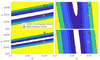 |
Fig. A.1. χ2 map of the X and Z scan for solar data. The orange and red crosses indicate the positions of AAG21 model including rotation and magnetic fields and the MB22 standard solar model respectively (values from their paper). The upper panels are associated with model M1 and the lower panels are associated with model A2 (see text for details). The left panels are associated with the high-T subdomain for the Z determination, while the right panels are associated with the low-T subdomain used to determine X. |
Appendix B: Solar data
Table B.1 summarises the sets of modes used in this paper. The full dataset is provided at the CDS. The BiSON data only covers low ℓ modes from zero to three, while the MDI data is for all higher degrees.
Datasets used in the inversion procedure.
All Tables
All Figures
|
Fig. 1. Left panel: profile of Γ1 between the BCZ and 0.95 R⊙ for the solar models in Table 1. Right panel: entropy proxy profile, P/ρΓ1, as a function of normalised radius for the solar models of Table 1. The reference evolutionary models (‘Ref’) show a significant spread in entropy proxy plateau in the CZ that is corrected in the seismic models (‘Seismic’) by the seismic reconstruction procedure. |
| In the text | |
|
Fig. 2. Details of the fitting approach used to determine the chemical composition of the solar envelope. The four-step process is tailored to eliminate cross-term contributions at each step and maximise the accuracy, while the last step computed a reduced χ2 value for each subdomain (see main text). |
| In the text | |
|
Fig. 3. Inversions of the Γ1 profile as a function of normalised radius for the artificial data (HH cases). Left panel: subdomain of the method for the Z determination (indicated by the orange vertical lines). Right panel: subdomain of the method for the X determination. |
| In the text | |
|
Fig. 4. Resulting χ2 map of the X and Z scan for the artificial data (HH exercises). The green and red crosses indicate the target and reference model, respectively. The upper panels are for HH1, middle panels are for HH2, and the lower panels are for HH3. The left panels are associated with the high-T subdomain for the Z determination, while the right panels are associated with the low-T subdomain used to determine X. |
| In the text | |
|
Fig. 5. Inversions of the Γ1 profile as a function of normalised radius determined from actual solar data. Left panel: subdomain of the method for the Z determination (indicated by the vertical orange lines). Right panel: subdomain of the method for the X determination. The orange curves are associated with reconstructions using FreeEOS, the purple curves are associated with reconstructions using SAHA-S, and the blue and red curves are associated with models M1 and M2 and A1 and A2, respectively. |
| In the text | |
|
Fig. 6. Resulting χ2 map of the X and Z scan for solar data using model A2 (upper panels), A3 (middle panel), and M2 (lower panels) in the procedure and using either SAHA-S v7 or SAHA-S v3. The orange and red crosses indicate the positions of the AAG21 model including rotation and magnetic fields and the MB22 standard solar model, respectively (values from their paper). The left panel is associated with the high-T subdomain for the Z determination, while the right panel is associated with the low-T subdomain used to determine X. |
| In the text | |
|
Fig. 7. Same as Fig. 6 for models A1 (upper panels) and M1 (lower panels), using FreeEOS in the reconstruction. The left panel is associated with the high-T subdomain for the Z determination, while the right panel is associated with the low-T subdomain used to determine X. |
| In the text | |
|
Fig. 8. Inversions of the Γ1 profile as a function of normalised radius determined from solar data assuming SAHA-S v7 as the EOS and changing the ratios of individual elements in the table (from MB22 to AAG21). Two reference models were used in the procedure: models M1 and A2. The results of the reconstructions are plotted in various colours. The red curve overplots the light blue one, and the purple curve overplots the green one. Each symbol depicts the Γ1 inversion results for the associated model (M1 or A2). |
| In the text | |
|
Fig. 9. Resulting χ2 map of the X and Z scan for the solar data fitting of Γ1 between 0.72 R⊙ and 0.91 R⊙. The orange crosses indicate the positions of the AAG21 model including rotation and magnetic fields, and the red crosses indicate the MB22 standard solar model (MB22-Phot in Table 2). Values are from their paper. The upper panels used the A2 model, and the lower panels used the M1 model. The left panels used MB22 individual elements, and the right panels used AAG21 individual elements. |
| In the text | |
|
Fig. 10. Inversions of the Γ1 profile as a function of normalised radius in the solar enveloped, determined using the Larson & Schou (2015) dataset. Left panel: subdomain of the method for the Z determination (indicated by the orange vertical lines). Right panel: subdomain of the method for the X determination. The green curve and symbols are associated with model M1 (FreeEOS), whereas the purple curve and symbols are associated with model A2 (SAHA-S v7). The red and blue lines illustrate models A1 and A2 and M1 and M2, respectively. |
| In the text | |
|
Fig. 11. Resulting χ2 map of the X and Z scan for solar data (Larson & Schou 2015) using model A2 in the procedure and fitting Γ1 between 0.72 R⊙ and 0.85 R⊙. The orange and red crosses indicate the positions of the AAG21 model including rotation and magnetic fields and the MB22 standard solar model, respectively (values from their paper). |
| In the text | |
|
Fig. 12. Summary of the inversion procedure for the various models, datasets, and EOSs. The green and red rectangles represent the intervals provided from the analysis of Sects. 4.2 and 4.4, respectively. The blue and red lines indicate the solar metallicity value from Magg et al. (2022; MB22) and Asplund et al. (2021; AAG21), respectively. |
| In the text | |
|
Fig. A.1. χ2 map of the X and Z scan for solar data. The orange and red crosses indicate the positions of AAG21 model including rotation and magnetic fields and the MB22 standard solar model respectively (values from their paper). The upper panels are associated with model M1 and the lower panels are associated with model A2 (see text for details). The left panels are associated with the high-T subdomain for the Z determination, while the right panels are associated with the low-T subdomain used to determine X. |
| In the text | |
Current usage metrics show cumulative count of Article Views (full-text article views including HTML views, PDF and ePub downloads, according to the available data) and Abstracts Views on Vision4Press platform.
Data correspond to usage on the plateform after 2015. The current usage metrics is available 48-96 hours after online publication and is updated daily on week days.
Initial download of the metrics may take a while.