| Issue |
A&A
Volume 686, June 2024
|
|
|---|---|---|
| Article Number | A108 | |
| Number of page(s) | 10 | |
| Section | The Sun and the Heliosphere | |
| DOI | https://doi.org/10.1051/0004-6361/202348312 | |
| Published online | 03 June 2024 | |
In-depth analysis of solar models with high-metallicity abundances and updated opacity tables
1
Département d’Astronomie, Université de Genève, Chemin Pegasi 51, 1290 Versoix, Switzerland
e-mail: This email address is being protected from spambots. You need JavaScript enabled to view it.
2
STAR Institute, Université de Liège, Liège, Belgium
3
Theoretical Astrophysics, Department of Physics and Astronomy, Uppsala University, Box 516 751 20 Uppsala, Sweden
4
Centre Spatial de Liège, Université de Liège, Angleur-Liège, Belgium
5
Los Alamos National Laboratory, Los Alamos, NM 87545, USA
6
Sternberg Astronomical Institute, Lomonosov Moscow State University, 119234 Moscow, Russia
Received:
18
October
2023
Accepted:
4
March
2024
Abstract
Context. As a result of the high-quality constraints available for the Sun, we are able to carry out detailed combined analyses using neutrino, spectroscopic, and helioseismic observations. These studies lay the ground for future improvements of the key physical components of solar and stellar models because ingredients such as the equation of state, the radiative opacities, or the prescriptions for macroscopic transport processes of chemicals are then used to study other stars in the Universe.
Aims. We study the existing degeneracies in solar models using the recent high-metallicity spectroscopic abundances by comparing them to helioseismic and neutrino data and discuss the effect on their properties of changes in the micro and macro physical ingredients.
Methods. We carried out a detailed study of solar models computed with a high-metallicity composition from the literature based on averaged 3D models that were claimed to resolve the solar modelling problem. We compared these models to helioseismic and neutrino constraints.
Results. The properties of the solar models are significantly affected by the use of the recent OPLIB opacity tables and the inclusion of macroscopic transport. The properties of the standard solar models computed using the OPAL opacities are similar to those for which the OP opacities were used. We show that a modification of the temperature gradient just below the base of the convective zone is required to remove the discrepancies in solar models, particularly in the presence of macroscopic mixing. This can be simulated by a localised increase in the opacity of a few percent.
Conclusions. We conclude that the existing degeneracies and issues in solar modelling are not removed by using an increase in the solar metallicity, in contradiction to what has been suggested in the recent literature. Therefore, standard solar models cannot be used as an argument for a high-metallicity composition. While further work is required to improve solar models, we note that direct helioseismic inversions indicate a low metallicity in the convective envelope, in agreement with spectroscopic analyses based on full 3D models.
Key words: Sun: abundances / Sun: fundamental parameters / Sun: helioseismology / Sun: oscillations
© The Authors 2024
 Open Access article, published by EDP Sciences, under the terms of the Creative Commons Attribution License (http://creativecommons.org/licenses/by/4.0), which permits unrestricted use, distribution, and reproduction in any medium, provided the original work is properly cited.
This article is published in open access under the Subscribe to Open model. This email address is being protected from spambots. You need JavaScript enabled to view it. to support open access publication.
1. Introduction
During the past 30 years, the solar metallicity, Z, has oscillated from a high to a low value, to again return to a high value in a recently published paper. The early works by Grevesse & Noels (1993, hereafter GN93) and Grevesse & Sauval (1998, hereafter GS98) led to values of Z/X = 0.0244 and Z/X = 0.0231, respectively. These results were obtained from analysing spectra taken at the centre of the solar disc using one dimension (1D) LTE photospheric models. More recently, new analyses of the same solar spectra that used new atomic data and improved 3D NLTE models by Asplund et al. (2009, hereafter AGSS09), Asplund et al. (2021, hereafter AAG21), and Amarsi et al. (2021) derived much lower metallicities, Z/X = 0.0181 and Z/X = 0.0187, respectively. Very recently, Magg et al. (2022, hereafter MB22) proposed a revision of the solar abundances leading to a metallicity of Z/X = 0.0226, which is a return to the high values of the 1990s and at 4.5σ with AAG21. This result was based on an analysis of the solar disc-integrated flux spectrum using a spatial and temporal average of a 3D RHD model, thus a 1D model called average 3D (⟨3D⟩). While further comparisons are required to fully understand the origin of the differences between the study of MB22 and those of AGSS09 and AAG21, it is interesting to briefly compare 3D and ⟨3D⟩ models, however. The differences between these two types of models are now well known: the 3D model outperforms the ⟨3D⟩ model by far, as is clearly observed when they are applied to the analysis of disc-integrated flux spectra, as shown in Fig. 7 of Amarsi et al. (2018) for the case of oxygen. The upward revision of the metallicity by MB22 has rekindled the debate about the so-called “solar problem”. As expected, their high-metallicity value improves the situation with neutrino measurements and some helioseismic constraints. However, the authors only computed one set of standard solar models to draw these conclusions and left a detailed analysis of the solar models to be performed later, arguing that the remaining discrepancies could be explained by remaining limitations of the stellar models and referring to Buldgen et al. (2019), who used AGSS09 as well as abundances based on the neon revision of Young (2018), and is therefore compatible with AAG21.
Recently, Buldgen et al. (2023) revised the claims of MB22 regarding the needs for revision of the physics of solar models. The authors showed that the agreement found by MB22 was due to a combination of physical ingredients and not based on the abundances alone. They discussed the appearance of various issues that arise when macroscopic transport of chemicals was included to reproduce the lithium depletion in the Sun, regardless of the parametrisation used for the transport coefficient. They also showed that an accurate determination of the solar beryllium abundance was required to fully characterise macroscopic transport at the base of the convective zone (BCZ). They mentioned that MB22 did not consider recent helioseismic determinations of the chemical composition of the solar envelope (Vorontsov et al. 2013; Buldgen et al. 2017a), which were further improved in precision (Buldgen et al. 2024), and in this last study provided an average over multiple reference models and datasets of Z = 0.0138. These independent approaches to determine the solar chemical composition confirm the low metallicity value of AAG21.
However, Buldgen et al. (2023) did not consider the impact of varying the reference opacity tables and combined helioseismic inversions and did not discuss the question of the remaining limitations mentioned in the conclusions of MB22. In this study, we use standard solar models (SSMs) and non-standard models including macroscopic mixing of chemicals using both the OPAL and OPLIB opacities and carry out a detailed investigation of calibrated models that were computed using the MB22 abundances in a similar way as Buldgen et al. (2019), who performed a detailed analysis like this using the AGSS09 abundances as well as the neon revision of Young (2018), which was later confirmed by AAG21. We thus significantly extend the set of solar models computed with the MB22 abundances and discuss our findings regarding global parameters such as the position of the BCZ, the helium mass fraction in the convective zone, neutrino fluxes and a combined helioseismic inversion of the squared adiabatic sound speed, the entropy proxy, and the Ledoux discriminant, as well as the frequency separation ratios of low-degree modes. We implemented a new diffusion coefficient to study macroscopic mixing below the convective envelope, derived from the asymptotic behaviour of the combined shear instability and magnetic Tayler instability in rotating solar models instead of the usual power law in density (see e.g. Proffitt & Michaud 1991; Richard et al. 1996; Christensen-Dalsgaard et al. 2018; Buldgen et al. 2023). This approach is linked to the solid-body rotation of the solar radiative interior (Brown et al. 1989; Thompson et al. 1996; Schou et al. 1998). As the inclusion of macroscopic transport reduces the extent of the solar convective zone, we also investigate the behaviour of solar models under the effects of adiabatic overshooting and a localised increase of opacities, which recover the helioseismic position of the base of the convective zone.
By combining all constraints available for the Sun, we carry out a detailed analysis of solar models using the MB22 abundances. We discuss the actual implications of the residual limitations of SSMs computed with revised high-metallicity solar abundances, and we disentangle the various contributors to these discrepancies in a similar way as Buldgen et al. (2019), taking macroscopic transport, localised opacity modifications, and overshooting at the base of the convective envelope into account. Our aim here is to further demonstrate the need for an improvement of the physics of solar models and to show that even when the MB22 abundances are taken at face value, our conclusions remain unchanged. Detailed helioseismic analyses of solar models built using these abundances combined with various opacity tables and a new formalism for macroscopic transport reinforce these needs and do not alleviate them.
2. Solar models
We computed solar models using the Liège stellar evolution code (Scuflaire et al. 2008) with various physical ingredients as in Buldgen et al. (2019). We used the recently suggested high-metallicity solar abundances (MB22) based on ⟨3D⟩ models, the latest version (v71) of the SAHA-S equation of state (Gryaznov et al. 2006, 2013). We refer to Buldgen et al. (2019) and references therein for similar comparisons between high- and low-metallicity solar models. We only discuss MB22 solar models here. Based on Buldgen et al. (2019) and from previous references, it appears that the two main ingredients affecting the properties of solar models are the transport of chemical elements and the opacity tables. In this study, we analyse the implication of the abundance revision by MB22 for various opacity tables available in the literature for the first time in detail. We thus compute the first MB22 standard solar models using the OPAL (Iglesias & Rogers 1996) and OPLIB (Colgan et al. 2016) opacity tables that were computed for this specific mixture, as well as models including macroscopic transport of chemicals reproducing the combined effects of hydrodynamic and magnetic instabilities due to the presence of rotation in the solar radiative zone (models denoted DR). We follow the work of Eggenberger et al. (2022), who computed solar models that reproduce both the lithium depletion and the internal rotation profile of the solar radiative zone. To do this, we use an asymptotic description of the transport coefficient of chemicals under the combined effects of meridional circulation, shear instability, and the magnetic Tayler instability (Spruit 2002).
As the Sun is a slow rotator, the dominant transport mechanism of chemicals due to rotation is the shear instability in the radiative layers of solar models, which results from the significant radial differential rotation (Zahn 1992). When the Tayler magnetic instability is included (Spruit 2002), the radial differential rotation is regulated via an efficient transport of angular momentum. However, a critical radial gradient of rotation is required for the instability to operate, and chemical gradients have an inhibiting effect on the apparition of this process. Therefore, the magnetic Tayler instability acts as an intermittent very efficient angular momentum transport that reduces the efficiency of the transport of chemicals by shear. We can thus estimate an asymptotic diffusion coefficient for the chemicals that is essentially the transport by shear, where the rotation gradient is the critical value at which the magnetic Tayler instability operates (since a larger radial rotation gradient would be quickly damped by the magnetic Tayler instability to the critical value).
Following this reasoning, we used the equation for the critical radial shear for the instability to operate,
 (1)
(1)
with Ω, the angular rotation velocity, assumed constant and fixed to the helioseismic value of the solar radiative zone, Nμ the chemical contribution to the Brunt–Väisälä frequency, and η the magnetic diffusivity, and we combined it with the vertical diffusion coefficient of the shear instability of Talon & Zahn (1997), DX, which consistently takes the effects of chemical composition gradients into account,
 (2)
(2)
with Dh the horizontal turbulence coefficient, Ric the critical Richardson number, dU/dz = r sin θ(dΩ/dr) the vertical shear rate, K the thermal diffusivity, and NT the thermal contribution to the Brunt–Väisälä frequency. The following expression for the macroscopic transport of chemicals is obtained after averaging over latitude:
 (3)
(3)
with f(r) a parametric function that is used to mimic the overall complex behaviour of the coefficient when the full transport of both angular momentum and chemicals was computed. The behaviour is, as expected, very similar to the recalibrated density power law used in Eggenberger et al. (2022). We mention, however, that this approach would need to be recalibrated in light of the incompatibility of the magnetic Tayler instability with the observations at later evolutionary stages (see e.g. Deheuvels et al. 2014, 2015; Gehan et al. 2018), particularly with the very young subgiants of Deheuvels et al. (2020). It would not impact the conclusions of our study, however, as they are similar to those of Buldgen et al. (2023)
We computed eight models in total because we also investigated the impact of replacing the position of the base of the convective zone at the helioseismically inferred value of 0.713 ± 0.001 R⊙ (Basu & Antia 1997) using either adiabatic convective penetration (denoted “Ov”) or a localised increase of opacity (denoted “OPAC”). We investigated whether one of these solutions was favoured over the other in the context of helioseismic inversions of the solar structure.
The increase in opacity was parametrised as follows:
 (4)
(4)
with κ0 the reference opacity of the model (e.g. either OPAL or OPLIB), and δκ the Gaussian opacity modification parametrised with temperature,
 (5)
(5)
with A the amplitude of the modification, and T the local temperature. The temperature we used was close to that of the Bailey et al. (2015) experiment, with an extension sufficient to affect the radiative layers, which were at slightly hotter temperatures in our models. The parametrisation was kept constant throughout the evolution of the solar model and led to a modification of the opacity profile at the BCZ that is illustrated in Fig. 1 for the OPAL model. Despite peaking in the convective zone (the BCZ is located at log T = 6.34), the modifications in the radiative layers just below the BCZ are still substantial and lead to significant differences in the helioseismic inference results.
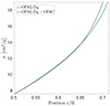 |
Fig. 1. Opacity profile as a function of the normalised radius for model OPAL DR (green) and model OPAL DR + OP (blue). |
2.1. Global parameters
We started by studying the relevant global parameters that describe solar models, namely the radial coordinate position of the base of the convective envelope, the mass coordinate at the position of the base of the convective envelope, the helium mass fraction in the convective envelope, and the photospheric lithium abundance. The values of these various parameters for each model are provided in Table 1.
Global parameters of the solar evolutionary models.
A first conclusion drawn from Table 1 is that the results of Buldgen et al. (2023) regarding the helium mass fraction in the convective envelope YCZ hold for the OPAL and OPLIB opacities. The OPAL tables were the reference opacity tables for the SSMs of the 1990s (e.g. Christensen-Dalsgaard et al. 1996), but they were replaced by the OP opacities (Badnell et al. 2005) in recent SSMs (Vinyoles et al. 2017). The recent OPLIB opacities are the latest generation of Los Alamos opacities. They were investigated in Colgan et al. (2016) and Buldgen et al. (2017b).
While the OPAL SSM in YCZ agrees excellently with the helioseismic measurement of YCZ, ⊙ = 0.2485 ± 0.0035 (Basu & Antia 1995), the values in models that include the effects of macroscopic mixing are too high with respect to the value inferred from helioseismology. We also note that a more recent determination by Vorontsov et al. (2013) using modern equations of state showed a slightly larger interval of values and favoured higher helium mass fraction values of about 0.25 in the CZ. This issue is still present in models for which the position of the base of the convective envelope is replaced at the helioseismic value (0.713 ± 0.001 R⊙) using either overshooting or an opacity increase. The inclusion of macroscopic mixing is required to reproduce the lithium photospheric abundance, A(Li) = 0.96 ± 0.05 dex (Wang et al. 2021), but it reduces the size of the solar convective envelope and thus destroys the existing agreement of high-metallicity models with helioseismology, as shown in Table 1. To restore this agreement, either an adiabatic convective penetration of 0.088 HP is applied at the BCZ (with HP the local pressure scale height), or an increase in opacity of 11% at the BCZ is applied (namely A = 0.12), following Eqs. (4) and (5).
The OPLIB models show a similar behaviour. However, because the OPLIB opacities are intrinsically lower than those of OPAL at a high temperature, the YCZ values of the models are shifted by about 0.005. This means that the OPLIB models that include macroscopic transport provide an overall better agreement than the OPAL models, in particular since they naturally lead to a deeper position of the base of the convective envelope. As discussed in Buldgen et al. (2023), the BCZ position is also significantly affected by the details of the formalism used to compute the microscopic diffusion of chemicals. This work as well as (Buldgen et al. 2019) showed that the effects of the screening coefficients of Paquette et al. (1986) are to push the BCZ position up by about 0.003.
Therefore, when the original implementation of Thoul et al. (1994) was used as in MB22, an SSM using the OPLIB opacities would have a slightly deeper position of the BCZ that almost disagrees with the helioseismic value. This clearly illustrates the degeneracy that exists in the solar models and the various parameters that can lead to agreement (or disagreement) with the extremely precise constraints for the Sun. Nevertheless, OPLIB models including macroscopic transport still need some increase in opacity or adiabatic convective penetration to replace the BCZ position at the helioseismic value. In this case, the convective penetration is only 0.061 HP, and the increase in opacity is 8.0% at the BCZ (or A = 0.085 in Eq. (5)).
2.2. Neutrino fluxes
The second relevant constraints to investigate when computing solar models are the neutrino fluxes. The results for our models are summarised in Table 2, where we illustrate the pp, Be, B, and CNO neutrino fluxes, denoted ϕ(pp), ϕ(B), ϕ(Be), and ϕ(CNO). We compare these results to the values provided in Borexino Collaboration (2018) and Orebi Gann et al. (2021).
Neutrino fluxes of the evolutionary models.
The first point we confirm is that high-metallicity SSMs computed with the OPAL opacities agree quite well with the Borexino fluxes, including the recent CNO fluxes of Appel et al. (2022). As shown in Table 2, we note that the analysis of Orebi Gann et al. (2021) provides a much lower ϕB value than Borexino, however, leading to a significant disagreement with the high-metallicity SSMs. As in Buldgen et al. (2023), the inclusion of macroscopic transport leads to a significant disagreement with the Borexino ϕB value that is often used to favour high CNO abundances in the Sun (Bahcall et al. 2005; Serenelli et al. 2013; Serenelli 2016; Borexino Collaboration 2018). In addition, the value of ϕCNO is now also much lower. It disagrees at 1σ with the measurements.
The issue is more tedious for the models computed with the OPLIB opacity tables. The SSM already disagrees at 1σ for the ϕCNO measurements as well as with the Borexino measurements of ϕB and ϕBe. When macroscopic mixing is added, the disagreement further increases, leading to questions about the properties of the solar core in the OPLIB models. The key parameter here is the lower opacity at high temperatures, which leads to a higher initial hydrogen abundance for the reproduction of the solar luminosity at the solar age. For a given solar metallicity, the helium abundance and central temperature is therefore lower, leading to a disagreement in neutrino fluxes and to a lower helium mass fraction in the CZ. This effect on the neutrino fluxes is further increased by the inclusion of the effects of macroscopic mixing, which has the tendency to push the calibration procedure towards even higher initial hydrogen abundances.
3. Helioseismic constraints
To fully investigate the helioseismic properties of our solar evolutionary models, we carried out seismic inversions of the squared adiabatic sound speed,  , with P the local pressure, ρ the local density, and
  the first adiabatic exponent, of the entropy proxy,
  and the Ledoux discriminant,
  . The combined analysis of these helioseismic inversions allowed us a clear view of the properties of solar models, as carried out in Buldgen et al. (2019), and it allowed us to investigate the individual contributions of some key elements of solar models in greater depth. We used the SOLA inversion technique (Pijpers & Thompson 1994), following the approach of Rabello-Soares et al. (1999), to calibrate the trade-off parameters.
3.1. Sound speed inversions
The squared adiabatic sound speed inversions for all models (SSMs and models including macroscopic transport) is illustrated in Fig. 2. When the reference opacity tables are varied for a given mixture, the impact is significant, as was illustrated in Buldgen et al. (2019) for the AGSS09 mixture. For the sound speed inversion alone, it might be argued that the OPLIB SSM is superior to the OPAL SSM, especially in the upper radiative layers. A similar situation was found for the GN93 abundances with the OPLIB tables. However, given the issues regarding the neutrino fluxes mentioned above, these conclusions are incomplete and do not encompass the whole picture. Similarly, the inclusion of macroscopic transport leads to a slight improvement of the agreement at the BCZ, but at the expense of increased discrepancies in the deeper layers. This is probably due to the reduction of the metallicity in the radiative zone.
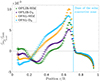 |
Fig. 2. Relative squared adiabatic sound speed differences between the Sun and models using the OPAL and OPLIB opacities, either within the standard solar model framework or including macroscopic mixing of chemical elements. |
In Fig. 3 we illustrate the impact of recovering the helioseismic value of 0.713 R⊙ of the BCZ using either adiabatic overshooting or a localised increase in the opacity. It appears that the two approaches are not equivalent, and the sound speed inversions would favour a localised opacity increase at the BCZ. Other results in the literature (e.g. Monteiro et al. 1994; Rempel 2004; Christensen-Dalsgaard et al. 2011; Zhang et al. 2019; Baraffe et al. 2022) show that a significant change in the temperature gradient on the radiative side is apparently favoured. Further investigations would be required to determine whether opacity modifications and effects of convective boundary mixing and thermalisation of the convective elements can be distinguished.
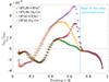 |
Fig. 3. Relative squared adiabatic sound speed differences between the Sun and models using the OPAL and OPLIB opacities, including macroscopic mixing of chemical elements and either adiabatic overshooting or a localised opacity increase to replace the BCZ at the helioseismic value. |
3.2. Entropy proxy inversions
The entropy proxy inversions for all SSMs and models including macroscopic mixing are illustrated in Fig. 4. Again, the best model seems to be the OPLIB SSM, which only shows small discrepancies throughout the radiative layers and a good agreement regarding the height of the entropy plateau in the CZ. This is in line with the conclusion of Buldgen et al. (2017b), who observed a similar trend for both AGSS09 and GN93 abundances when comparing OPAL to OPLIB models. The inclusion of macroscopic transport significantly improves the agreement around 0.6 R⊙ for the OPLIB model by essentially erasing the contribution of mean molecular weight gradients to this quantity. The situation is exactly the opposite for the OPAL model, as macroscopic transport leads to significiant discrepancies. The position of the entropy plateau in the CZ with macroscopic transport agrees less well by about 0.003, which is still significant at our precision level. It appears that none of the models, standard or otherwise, is able to place the entropy plateau at the correct height. In the deeper radiative layers and in the core, the changes remain quite small and are similar to the sound speed variations overall.
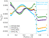 |
Fig. 4. Differences in the relative entropy proxy between the Sun and models using the OPAL and OPLIB opacities, either within the standard solar model framework or including macroscopic mixing of chemical elements. |
As for the sound speed inversion, the entropy proxy traces how the position of the base of the convective envelope is replaced. It appears that a localised opacity modification improves the height of the entropy plateau by about 0.005, but worsens the agreement just below the BCZ by about 0.6 R⊙ (see Fig. 5). This conclusion is reached for both OPAL and OPLIB opacity tables and is likely due to the shape of the opacity modification. Adiabatic overshooting does not affect the height of the entropy plateau at all, however. In the case of the AGSS09 abundances, Buldgen et al. (2019) found that when adiabatic overshooting extends deep enough, the height of the plateau in one of their models could be strongly affected, but the sound speed inversion results were then significantly worse. This implies that the temperature gradient in the radiative layers is poorly described with the current approach, but that some degree of steepening is required to place the plateau in the CZ at the correct height. This contradicts the sound speed profile inversions that would strictly favour a model using the opacity modification of Eq. (4).
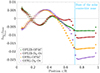 |
Fig. 5. Relative entropy proxy differences between the Sun and models using the OPAL and OPLIB opacities, including macroscopic mixing of chemical elements and either adiabatic overshooting or a localised opacity increase to replace the BCZ at the helioseismic value. |
Based on the entropy proxy inversions, the situation appears far more complex, despite the revision of the abundances by MB22, which improved the agreement from the point of view of the sound speed profile.
3.3. Ledoux discriminant inversions
The last inversion we investigated is that of the Ledoux discriminant profile, which amplifies the discrepancies at the BCZ. Figure 6 shows that the OPLIB SSM is only superior to that of OPAL close to the BCZ. In a similar way to what was observed for the GN93 abundances in Buldgen et al. (2017c), there seems to be a region, around 0.6 R⊙, where the temperature gradient is too steep in the OPLIB model. This can be due to a too high opacity in these layers as a result of the higher oxygen and iron abundance. This discrepancy is located very close to the peak in metallicity that is observed in the SSMs due to the competing effects of pressure and thermal diffusion, which in turn induce a higher opacity as the metals are the most dominant contributors at these temperatures (Blancard et al. 2012). The inclusion of macroscopic mixing erases this peak in metallicity and thus leads to a much fainter temperature gradient. For the OPLIB model, this significantly improves the agreement around 0.6 R⊙, but the improvement is much smaller for the OPAL model. The sharp variations at the base of the convective zone are slightly reduced by macroscopic mixing, indicating that a fainter chemical composition gradient is favoured, in agreement with previous studies (e.g. Brun et al. 2002; Takata & Shibahashi 2003; Baturin et al. 2015; Christensen-Dalsgaard et al. 2018).
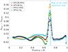 |
Fig. 6. Ledoux discriminant differences between the Sun and models using the OPAL and OPLIB opacities, either within the standard solar model framework or including macroscopic mixing of chemical elements. |
The effects of including adiabatic overshooting and a localised increase in opacity are illustrated in Fig. 7. Again, both effects can be easily distinguished. In both cases, the opacity increase efficiently reduces the sharp peak at the BCZ. The OPLIB model with the opacity increase is again favoured, while the OPAL model with the opacity increase shows a quite extended deviation in the bulk of the radiative zone. This is due to the exact shape of the opacity profile in the model, which extends to slightly higher temperatures in this case. The amplitude of the opacity modification was increased from 8.5% to 12% between the OPLIB and the OPAL model, but the width of the Gaussian function remained the same. Therefore, the amplitude remains slightly larger at higher temperatures and explains the deviations, as illustrated in Fig. 1. This demonstrates both that opacity modifications should remain very localised in these models and that the Ledoux discriminant inversion is extremely efficient at constraining the temperature gradient in the upper solar radiative layers.
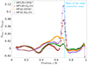 |
Fig. 7. Ledoux discriminant differences between the Sun and models using the OPAL and OPLIB opacities, including macroscopic mixing of chemical elements and either adiabatic overshooting or a localised opacity increase to replace the BCZ at the helioseismic value. |
3.4. Frequency separation ratios
The frequency separation ratios defined by Roxburgh & Vorontsov (2003) are classical constraints in helioseismology. They have been used in numerous discussions related to the solar abundances (e.g. Basu et al. 2007; Chaplin et al. 2007) and the physics of solar models (Buldgen et al. 2017b; Salmon et al. 2021). They serve as a direct test of the sound speed gradient in the deep solar layers (Roxburgh & Vorontsov 2003), as can be shown using asymptotic developments (Shibahashi 1979; Tassoul 1980) that they satisfy the following relation:
 (6)
(6)
with c the adiabatic sound speed defined above, ℓ the degree of the mode, and R the solar radius. This constraint is regularly used for the asteroseismic modelling of solar-like oscillators, but also as a straightforward test of solar models.
Therefore, we computed the frequency separation ratios for all the models in this study and compared them to an SSM using the GN93 abundances, FreeEOS, and OPAL opacities, which would be the reference of the 1990s to reproduce. To better illustrate the level of agreement, we compared the following quantity:
 (7)
(7)
with σrn, ℓ the uncertainty on the observed frequency separation ratios. This quantity has the advantage of directly showing how significant the differences are. However, it should be kept in mind that the very high precision of the solar data implies that almost no model reaches a 1σ level of agreement for all frequency separation ratios.
These results are illustrated in Fig. 8 for the standard solar models and for models with the revised turbulent formalism. Figure 9 shows the models with both macroscopic transport and overshooting or an opacity modification. According to Figs. 8 and 9, none of the models performs quite well, regardless of the opacity table that is used for them. When we compare the MB22 models to the GN93 model, we can clearly see that their level of agreement is significantly lower, particularly at low and intermediate frequencies, for both OPLIB and OPAL opacities, even when the BCZ position is replaced using overshooting or an opacity increase.
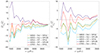 |
Fig. 8. Frequency separation ratios as a function of frequency of standard solar models and models including macroscopic mixing described in Table 1, compared to BiSON low-degree data. A standard solar model using the GN93 abundances is also shown in comparison. |
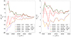 |
Fig. 9. Frequency separation ratios as a function of frequency of models including macroscopic mixing and an localised opacity increase or convective overshooting at the BCZ described in Table 1, compared to BiSON low-degree data. A standard solar model using the GN93 abundances is also shown in comparison. |
This situation is in clear contrast with the agreement found for higher-metallicity models of the 90s (see e.g. Chaplin et al. 2007; Basu et al. 2007; Serenelli et al. 2009; Buldgen et al. 2017b). Due to the similarities between the OP and the OPAL opacities, the same level of agreement was found when the experiment was repeated with an OP model. Further investigations regarding the exact layers to which the frequency separation ratios and their slope are sensitive might help determine the exact origins of the observed deviations. The AGSS09 models using the OPLIB opacities are found to provide a good agreement, but clearly disagree for other key constraints such as neutrino fluxes and the helium abundance in the convective zone (see Buldgen et al. 2017b; Salmon et al. 2021, and the associated discussion).
4. Discussion
The immediate result of our detailed analysis of solar models with revised MB22 abundances is that the agreement found for SSMs strongly depends on the radiative opacities used to compute them. While models using OPAL tables agree excellently with helioseismic and neutrino data, models using OPLIB tables show significant discrepancies in neutrino fluxes while showing a better agreement with helioseismic constraints overall, with the exception of the helium mass fraction in the CZ. This issue regarding the OPLIB tables was already discussed in Buldgen et al. (2019) and Salmon et al. (2021), and detailed comparisons are required to determine the origin of the differences between OPAL, OP, and OPLIB. Similarly, the good performance of the OPAL opacities are expected because the differences between OPAL and OP are small. Therefore, even for SSMs, a detailed analysis of the models leads us to conclude that despite the improvements due to the increase in the solar abundances, key issues remain linked to the current state of solar modelling. In this context, the existing degeneracies in classical helioseismic inferences cannot be used to validate abundance determinations. The conclusions we draw from the OPAL models can thus be applied to the OP models because the two opacity tables are similar. A striking issue is also found for the frequency separation ratios, which only provide a moderate agreement with solar models using the MB22 abundances. This is far from what was achieved with GS98 or GN93 models. In this respect the MB22 abundances are not exactly equivalent to the GS98 abundances. Further investigations are required to examine exactly from where these discrepancies arise.
The second main result is that the situation drastically changes when macroscopic mixing is taken into account to reproduce the lithium depletion at the solar surface. This has been discussed in Buldgen et al. (2023) and was generalised here to models including the OPAL and OPLIB opacities. The significant decrease in neutrino fluxes observed for models including macroscopic mixing is due the drastic change in the calibration results when we attempted to reproduce the lithium observations. As mentioned in Buldgen et al. (2023), a reliable beryllium determination would be required to further constrain the efficiency of macroscopic mixing at the BCZ. The impact of planetary formation could mitigate the issue (Kunitomo et al. 2022), but modifications to other key physical ingredients such as opacity at higher temperatures and electronic screening (Mussack & Däppen 2011; Mussack 2011) cannot be excluded.
The third main result is linked to the effect of macroscopic mixing on the position of the BCZ and its effect on key indicators of thermal gradients such as the entropy plateau in the CZ and the Ledoux discriminant. We confirm that helioseismic data strongly favour significant modifications of the thermal gradients in the radiative zone even with revised abundances. Replacing the BCZ to the helioseismic value of 0.713 R⊙ using adiabatic overshooting does not significantly improve the agreement of the models with helioseismic inferences, whereas a localised increase in the opacity decreases the observed discrepancies. Whether the changes in the temperature gradients can be due to the thermalisation of the convective elements in the radiative zone remains to be explored using physically motivated prescriptions (Baraffe et al. 2022). However, a key difference between an opacity increase and effects linked to convective overshooting resides in the mixing of chemical elements and the potential impact on the lithium and beryllium depletion. On the other hand, the opacity modification implemented here is not entirely realistic because an actual revision of opacities might lead to significant changes in opacity at higher temperatures, as was seen for the OPAS and OPLIB tables and as can be expected from new computations (e.g. Nahar & Pradhan 2016; Zhao et al. 2018; Pain & Gilleron 2020; Pradhan & Nahar 2018; Pradhan 2023).
Overall, the situation appears to be quite complex and still requires extensive investigations. While uncertainties between the various opacity tables are a concern, the dispersion of 0.6 dex inferred by MB22 for iron (Table A.1), which was not described by Asplund et al. (2021), significantly worsens the situation as this element, together with oxygen, is the first contributor to opacity at the BCZ and remains highly significant throughout the solar radiative zone. Given the uncertainties on iron opacity (Bailey et al. 2015) and the impact of new physical processes in the computations (Pradhan 2023), a detailed discussion of these discrepancies is required before a definitive conclusion regarding solar models can be reached. Further analyses using linear solar models (Villante & Ricci 2010), seismic models (Buldgen et al. 2020), or extended calibration procedures (Ayukov & Baturin 2017; Kunitomo & Guillot 2021) might be informative, but these will have to be combined with theoretical inputs to lift the degeneracies that appear when non-standard solar models are used in the solar calibration procedure. No such degeneracies are present in the SSM calibration that used a simplified physical picture.
5. Conclusion
We have analyzed in detail solar models computed with the abundances proposed by MB22. We investigated the effects of changing the opacity tables within the SSM framework, including macroscopic mixing at the BCZ mimicking the effects of rotating models (Eggenberger et al. 2022), and we then added the adiabatic overshooting or a localised opacity increase to compensate for the effects of macroscopic mixing on the position of the BCZ. A complete picture of the situation was drawn by studying the global properties and neutrino fluxes of the models in Sect. 2 as well as combined helioseismic inversions in Sect. 3. The results were discussed in Sect. 4, where three main points of discussion are outlined.
We conclude that the proposed revision of the solar abundances by MB22 does not change the need for future improvements of solar models. While MB22 considered that the remaining discrepancies can be solved using investigations following Buldgen et al. (2019), we showed in this study that this is not the case. On the contrary, it appears that the good agreement regarding sound speed, neutrino fluxes, and global parameters found by MB22 for their SSMs is due to a favourable combination of physical ingredients of their models. Like for a tightrope walker, a small push in a given direction worsens the situation for the SSMs. For example, changing the radiative opacities or including macroscopic transport leads to an overall worsening of the situation regarding helium, neutrino fluxes, or the BCZ position while significantly changing the results of helioseismic inferences, and not always for the better. In addition, choices regarding spectral lines, datasets, and microphysical ingredients in the spectroscopic analysis by MB22 need to be discussed, as well as the extreme spread in iron abundance they find, which would drastically change the properties of solar models.
A clear difference between low- and high-z solar models is that further improvements of the physics of the models, such as an opacity increase motivated by recent works or the inclusion of light-element depletion, tend to reduce some of the discrepancies in low-z models, while they increase them in high-z models. This is to be placed in perspective in the context of recent solar envelope metallicity determinations (Vorontsov et al. 2013; Buldgen et al. 2017a, 2024), which tend to be consistent with AAG21 spectrosopic values, leaving the differences with MB22 to be explained.
As outlined in Buldgen et al. (2019), renewed detailed analyses of solar models are required to determine the importance of numerical uncertainties in the comparisons of solar models with the highly precise constraints available for the Sun. In parallel, experimental efforts for more precise determinations of CNO neutrino fluxes as well as experimental and theoretical opacity values in solar conditions remain key factors to constrain the deep radiative interior of solar models. Regarding the solar convective layers and the BCZ interface, our work showed that combining helioseismic inversions to light element depletion might provide a data-driven analysis of both the chemical and thermal properties of the BCZ. Further improvements to the resolution of the inversion techniques, by using non-linear RLS methods (Corbard et al. 1999), might be required to obtain a full picture, however.
Acknowledgments
We thank the referee for their thorough reading of the manuscript. G.B. is funded by the SNF AMBIZIONE grant No. 185805 (Seismic inversions and modelling of transport processes in stars). A.M.A. gratefully acknowledges support from the Swedish Research Council (VR 2020-03940). P.E. received funding from the European Research Council (ERC) under the European Union’s Horizon 2020 research and innovation programme (grant agreement No. 833925, project STAREX). We acknowledge support by the ISSI team “Probing the core of the Sun and the stars” (ID 423) led by Thierry Appourchaux.
References
- Amarsi, A. M., Barklem, P. S., Asplund, M., Collet, R., & Zatsarinny, O. 2018, A&A, 616, A89 [NASA ADS] [CrossRef] [EDP Sciences] [Google Scholar]
- Amarsi, A. M., Grevesse, N., Asplund, M., & Collet, R. 2021, A&A, 656, A113 [NASA ADS] [CrossRef] [EDP Sciences] [Google Scholar]
- Appel, S., Bagdasarian, Z., Basilico, D., et al. 2022, Phys. Rev. Lett., 129, 252701 [NASA ADS] [CrossRef] [Google Scholar]
- Asplund, M., Grevesse, N., Sauval, A. J., & Scott, P. 2009, ARA&A, 47, 481 [NASA ADS] [CrossRef] [Google Scholar]
- Asplund, M., Amarsi, A. M., & Grevesse, N. 2021, A&A, 653, A141 [NASA ADS] [CrossRef] [EDP Sciences] [Google Scholar]
- Ayukov, S. V., & Baturin, V. A. 2017, Astron. Rep., 61, 901 [NASA ADS] [CrossRef] [Google Scholar]
- Badnell, N. R., Bautista, M. A., Butler, K., et al. 2005, MNRAS, 360, 458 [Google Scholar]
- Bahcall, J. N., Basu, S., Pinsonneault, M., & Serenelli, A. M. 2005, ApJ, 618, 1049 [NASA ADS] [CrossRef] [Google Scholar]
- Bailey, J. E., Nagayama, T., Loisel, G. P., et al. 2015, Nature, 517, 3 [Google Scholar]
- Baraffe, I., Constantino, T., Clarke, J., et al. 2022, A&A, 659, A53 [NASA ADS] [CrossRef] [EDP Sciences] [Google Scholar]
- Basu, S., & Antia, H. M. 1995, MNRAS, 276, 1402 [NASA ADS] [Google Scholar]
- Basu, S., & Antia, H. M. 1997, MNRAS, 287, 189 [NASA ADS] [CrossRef] [Google Scholar]
- Basu, S., Chaplin, W. J., Elsworth, Y., et al. 2007, ApJ, 655, 660 [NASA ADS] [CrossRef] [Google Scholar]
- Baturin, V. A., Gorshkov, A. B., & Oreshina, A. V. 2015, Astron. Rep., 59, 46 [NASA ADS] [CrossRef] [Google Scholar]
- Blancard, C., Cossé, P., & Faussurier, G. 2012, ApJ, 745, 10 [NASA ADS] [CrossRef] [Google Scholar]
- Borexino Collaboration (Agostini, M., et al.) 2018, Nature, 562, 505 [CrossRef] [Google Scholar]
- Borexino Collaboration (Agostini, M., et al.) 2020, Nature, 587, 577 [NASA ADS] [CrossRef] [Google Scholar]
- Brown, T. M., Christensen-Dalsgaard, J., Dziembowski, W. A., et al. 1989, ApJ, 343, 526 [Google Scholar]
- Brun, A. S., Antia, H. M., Chitre, S. M., & Zahn, J. P. 2002, A&A, 391, 725 [NASA ADS] [CrossRef] [EDP Sciences] [Google Scholar]
- Buldgen, G., Salmon, S. J. A. J., Noels, A., et al. 2017a, MNRAS, 472, 751 [NASA ADS] [CrossRef] [Google Scholar]
- Buldgen, G., Salmon, S. J. A. J., Noels, A., et al. 2017b, A&A, 607, A58 [NASA ADS] [CrossRef] [EDP Sciences] [Google Scholar]
- Buldgen, G., Salmon, S. J. A. J., Godart, M., et al. 2017c, MNRAS, 472, L70 [NASA ADS] [CrossRef] [Google Scholar]
- Buldgen, G., Salmon, S. J. A. J., Noels, A., et al. 2019, A&A, 621, A33 [NASA ADS] [CrossRef] [EDP Sciences] [Google Scholar]
- Buldgen, G., Eggenberger, P., Baturin, V. A., et al. 2020, A&A, 642, A36 [EDP Sciences] [Google Scholar]
- Buldgen, G., Eggenberger, P., Noels, A., et al. 2023, A&A, 669, L9 [NASA ADS] [CrossRef] [EDP Sciences] [Google Scholar]
- Buldgen, G., Noels, A., Baturin, V. A., et al. 2024, A&A, 681, A57 [NASA ADS] [CrossRef] [EDP Sciences] [Google Scholar]
- Chaplin, W. J., Serenelli, A. M., Basu, S., et al. 2007, ApJ, 670, 872 [NASA ADS] [CrossRef] [Google Scholar]
- Christensen-Dalsgaard, J., Dappen, W., Ajukov, S. V., et al. 1996, Science, 272, 1286 [Google Scholar]
- Christensen-Dalsgaard, J., Monteiro, M. J. P. F. G., Rempel, M., & Thompson, M. J. 2011, MNRAS, 414, 1158 [CrossRef] [Google Scholar]
- Christensen-Dalsgaard, J., Gough, D. O., & Knudstrup, E. 2018, MNRAS, 477, 3845 [CrossRef] [Google Scholar]
- Colgan, J., Kilcrease, D. P., Magee, N. H., et al. 2016, ApJ, 817, 116 [Google Scholar]
- Corbard, T., Blanc-Féraud, L., Berthomieu, G., & Provost, J. 1999, A&A, 344, 696 [NASA ADS] [Google Scholar]
- Deheuvels, S., Doğan, G., Goupil, M. J., et al. 2014, A&A, 564, A27 [NASA ADS] [CrossRef] [EDP Sciences] [Google Scholar]
- Deheuvels, S., Ballot, J., Beck, P. G., et al. 2015, A&A, 580, A96 [NASA ADS] [CrossRef] [EDP Sciences] [Google Scholar]
- Deheuvels, S., Ballot, J., Eggenberger, P., et al. 2020, A&A, 641, A117 [EDP Sciences] [Google Scholar]
- Eggenberger, P., Buldgen, G., Salmon, S. J. A. J., et al. 2022, Nat. Astron., 6, 788 [NASA ADS] [CrossRef] [Google Scholar]
- Gehan, C., Mosser, B., Michel, E., Samadi, R., & Kallinger, T. 2018, A&A, 616, A24 [NASA ADS] [CrossRef] [EDP Sciences] [Google Scholar]
- Grevesse, N., & Noels, A. 1993, in Origin and Evolution of the Elements, eds. N. Prantzos, E. Vangioni-Flam, & M. Casse, 15 [Google Scholar]
- Grevesse, N., & Sauval, A. J. 1998, Space Sci. Rev., 85, 161 [Google Scholar]
- Gryaznov, V. K., Ayukov, S. V., Baturin, V. A., et al. 2006, J. Phys. A Math. Gen., 39, 4459 [NASA ADS] [CrossRef] [Google Scholar]
- Gryaznov, V. K., Iosilevskiy, I. L., Fortov, V. E., et al. 2013, Contrib. Plasma Phys., 53, 392 [NASA ADS] [CrossRef] [Google Scholar]
- Iglesias, C. A., & Rogers, F. J. 1996, ApJ, 464, 943 [NASA ADS] [CrossRef] [Google Scholar]
- Kunitomo, M., & Guillot, T. 2021, A&A, 655, A51 [NASA ADS] [CrossRef] [EDP Sciences] [Google Scholar]
- Kunitomo, M., Guillot, T., & Buldgen, G. 2022, A&A, 667, L2 [NASA ADS] [CrossRef] [EDP Sciences] [Google Scholar]
- Magg, E., Bergemann, M., Serenelli, A., et al. 2022, A&A, 661, A140 [NASA ADS] [CrossRef] [EDP Sciences] [Google Scholar]
- Monteiro, M. J. P. F. G., Christensen-Dalsgaard, J., & Thompson, M. J. 1994, A&A, 283, 247 [NASA ADS] [Google Scholar]
- Mussack, K. 2011, Ap&SS, 336, 111 [CrossRef] [Google Scholar]
- Mussack, K., & Däppen, W. 2011, ApJ, 729, 96 [Google Scholar]
- Nahar, S. N., & Pradhan, A. K. 2016, Phys. Rev. Lett., 116, 235003 [Google Scholar]
- Orebi Gann, G. D., Zuber, K., Bemmerer, D., & Serenelli, A. 2021, Annu. Rev. Nucl. Part. Sci., 71, 491 [CrossRef] [Google Scholar]
- Pain, J.-C., & Gilleron, F. 2020, High Energy Density Phys., 34, 100745 [NASA ADS] [CrossRef] [Google Scholar]
- Paquette, C., Pelletier, C., Fontaine, G., & Michaud, G. 1986, ApJS, 61, 177 [Google Scholar]
- Pijpers, F. P., & Thompson, M. J. 1994, A&A, 281, 231 [NASA ADS] [Google Scholar]
- Pradhan, A. 2023, arXiv e-prints [arXiv:2301.07734] [Google Scholar]
- Pradhan, A. K., & Nahar, S. N. 2018, ASP Conf. Ser., 515, 79 [NASA ADS] [Google Scholar]
- Proffitt, C. R., & Michaud, G. 1991, ApJ, 380, 238 [Google Scholar]
- Rabello-Soares, M. C., Basu, S., & Christensen-Dalsgaard, J. 1999, MNRAS, 309, 35 [NASA ADS] [CrossRef] [Google Scholar]
- Rempel, M. 2004, ApJ, 607, 1046 [Google Scholar]
- Richard, O., Vauclair, S., Charbonnel, C., & Dziembowski, W. A. 1996, A&A, 312, 1000 [NASA ADS] [Google Scholar]
- Roxburgh, I. W., & Vorontsov, S. V. 2003, A&A, 411, 215 [NASA ADS] [CrossRef] [EDP Sciences] [Google Scholar]
- Salmon, S. J. A. J., Buldgen, G., Noels, A., et al. 2021, A&A, 651, A106 [NASA ADS] [CrossRef] [EDP Sciences] [Google Scholar]
- Schou, J., Antia, H. M., Basu, S., et al. 1998, ApJ, 505, 390 [Google Scholar]
- Scuflaire, R., Théado, S., Montalbán, J., et al. 2008, Ap&SS, 316, 83 [Google Scholar]
- Serenelli, A. 2016, Eur. Phys. J. A, 52, 78 [CrossRef] [Google Scholar]
- Serenelli, A. M., Basu, S., Ferguson, J. W., & Asplund, M. 2009, ApJ, 705, L123 [Google Scholar]
- Serenelli, A., Peña-Garay, C., & Haxton, W. C. 2013, Phys. Rev. D, 87, 043001 [Google Scholar]
- Shibahashi, H. 1979, PASJ, 31, 87 [NASA ADS] [Google Scholar]
- Spruit, H. C. 2002, A&A, 381, 923 [CrossRef] [EDP Sciences] [Google Scholar]
- Takata, M., & Shibahashi, H. 2003, PASJ, 55, 1015 [NASA ADS] [CrossRef] [Google Scholar]
- Talon, S., & Zahn, J. P. 1997, A&A, 317, 749 [NASA ADS] [Google Scholar]
- Tassoul, M. 1980, ApJS, 43, 469 [Google Scholar]
- Thompson, M. J., Toomre, J., Anderson, E. R., et al. 1996, Science, 272, 1300 [Google Scholar]
- Thoul, A. A., Bahcall, J. N., & Loeb, A. 1994, ApJ, 421, 828 [Google Scholar]
- Villante, F. L., & Ricci, B. 2010, ApJ, 714, 944 [NASA ADS] [CrossRef] [Google Scholar]
- Vinyoles, N., Serenelli, A. M., Villante, F. L., et al. 2017, ApJ, 835, 202 [NASA ADS] [CrossRef] [Google Scholar]
- Vorontsov, S. V., Baturin, V. A., Ayukov, S. V., & Gryaznov, V. K. 2013, MNRAS, 430, 1636 [Google Scholar]
- Wang, E. X., Nordlander, T., Asplund, M., et al. 2021, MNRAS, 500, 2159 [Google Scholar]
- Young, P. R. 2018, ApJ, 855, 15 [Google Scholar]
- Zahn, J. P. 1992, A&A, 265, 115 [NASA ADS] [Google Scholar]
- Zhang, Q.-S., Li, Y., & Christensen-Dalsgaard, J. 2019, ApJ, 881, 103 [Google Scholar]
- Zhao, L., Eissner, W., Nahar, S. N., & Pradhan, A. K. 2018, ASP Conf. Ser., 515, 89 [NASA ADS] [Google Scholar]
All Tables
All Figures
|
Fig. 1. Opacity profile as a function of the normalised radius for model OPAL DR (green) and model OPAL DR + OP (blue). |
| In the text | |
|
Fig. 2. Relative squared adiabatic sound speed differences between the Sun and models using the OPAL and OPLIB opacities, either within the standard solar model framework or including macroscopic mixing of chemical elements. |
| In the text | |
|
Fig. 3. Relative squared adiabatic sound speed differences between the Sun and models using the OPAL and OPLIB opacities, including macroscopic mixing of chemical elements and either adiabatic overshooting or a localised opacity increase to replace the BCZ at the helioseismic value. |
| In the text | |
|
Fig. 4. Differences in the relative entropy proxy between the Sun and models using the OPAL and OPLIB opacities, either within the standard solar model framework or including macroscopic mixing of chemical elements. |
| In the text | |
|
Fig. 5. Relative entropy proxy differences between the Sun and models using the OPAL and OPLIB opacities, including macroscopic mixing of chemical elements and either adiabatic overshooting or a localised opacity increase to replace the BCZ at the helioseismic value. |
| In the text | |
|
Fig. 6. Ledoux discriminant differences between the Sun and models using the OPAL and OPLIB opacities, either within the standard solar model framework or including macroscopic mixing of chemical elements. |
| In the text | |
|
Fig. 7. Ledoux discriminant differences between the Sun and models using the OPAL and OPLIB opacities, including macroscopic mixing of chemical elements and either adiabatic overshooting or a localised opacity increase to replace the BCZ at the helioseismic value. |
| In the text | |
|
Fig. 8. Frequency separation ratios as a function of frequency of standard solar models and models including macroscopic mixing described in Table 1, compared to BiSON low-degree data. A standard solar model using the GN93 abundances is also shown in comparison. |
| In the text | |
|
Fig. 9. Frequency separation ratios as a function of frequency of models including macroscopic mixing and an localised opacity increase or convective overshooting at the BCZ described in Table 1, compared to BiSON low-degree data. A standard solar model using the GN93 abundances is also shown in comparison. |
| In the text | |
Current usage metrics show cumulative count of Article Views (full-text article views including HTML views, PDF and ePub downloads, according to the available data) and Abstracts Views on Vision4Press platform.
Data correspond to usage on the plateform after 2015. The current usage metrics is available 48-96 hours after online publication and is updated daily on week days.
Initial download of the metrics may take a while.