| Issue |
A&A
Volume 694, February 2025
|
|
|---|---|---|
| Article Number | A285 | |
| Number of page(s) | 10 | |
| Section | The Sun and the Heliosphere | |
| DOI | https://doi.org/10.1051/0004-6361/202452918 | |
| Published online | 20 February 2025 | |
Constraints on the properties of macroscopic transport in the Sun from combined lithium and beryllium depletion
1
STAR Institute, Université de Liège, Liège, Belgium
2
Theoretical Astrophysics, Department of Physics and Astronomy, Uppsala University, Box 516 751 20 Uppsala, Sweden
3
University of Virginia, Astronomy Building, 530 McCormick Road, PO Box 400325 Charlottesville, VA 22904, USA
4
LUPM, Université de Montpellier, CNRS, Place Eugène Bataillon, 34095 Montpellier, France
5
Centre Spatial de Liège, Université de Liège, Angleur-Liège, Belgium
⋆ Corresponding author; This email address is being protected from spambots. You need JavaScript enabled to view it.
Received:
7
November
2024
Accepted:
6
January
2025
Abstract
Context. The Sun is a privileged laboratory of stellar evolution, thanks to the quality and complementary nature of available constraints. Using these observations, we are able to draw a detailed picture of its internal structure and dynamics, which forms the basis of the successes of solar modelling. Amongst such observations, constraints on the depletion of lithium and beryllium are key tracers of the required efficiency and extent of macroscopic mixing just below the solar convective envelope. Thanks to revised determinations of these abundances, we may use them in conjunction with other existing spectroscopic and helioseismic constraints to study in detail the properties of macroscopic transport.
Aims. We aim to constrain the efficiency of macroscopic transport at the base of the solar convective zone (BCZ) and determining the compatibility of the observations with a suggested candidate linked with the transport of angular momentum in the solar radiative interior.
Methods. We use recent spectroscopic observations of lithium and beryllium abundance and include them in solar evolutionary model calibrations. We test the agreement of such models in terms of position of the convective envelope, helium mass fraction in the convective zone, sound speed profile inversions, and neutrino fluxes.
Results.We constrain the required efficiency and extent of the macroscopic mixing at the base of the BCZ, finding that a power-law density with an index, n, between 3 and 6 would reproduce the data, with efficiencies at the BCZ of about 6000 cm2/s, depending on the value of n. We also confirm that macroscopic mixing worsens the agreement with neutrino fluxes and that the current implementations of the magnetic Tayler instability are unable to explain the observations.
Key words: Sun: abundances / Sun: fundamental parameters / Sun: helioseismology / Sun: oscillations
© The Authors 2025
 Open Access article, published by EDP Sciences, under the terms of the Creative Commons Attribution License (https://creativecommons.org/licenses/by/4.0), which permits unrestricted use, distribution, and reproduction in any medium, provided the original work is properly cited.
This article is published in open access under the Subscribe to Open model. This email address is being protected from spambots. You need JavaScript enabled to view it. to support open access publication.
1. Introduction
The Sun is a crucial laboratory of stellar physics at microscopic and macroscopic scales and an important reference point for stellar evolution in general (see Christensen-Dalsgaard 2021, and references therein). Thanks to helioseismic and spectroscopic constraints, supplemented by the detections of neutrinos directly informing us on the properties of the solar core, we are able to draw a detailed picture of the internal structure and dynamics of the Sun (see e.g. Christensen-Dalsgaard et al. 1991, 1996; Basu & Antia 1995, 1997; Basu et al. 2009; Schou et al. 1998; Orebi Gann et al. 2021; Appel et al. 2022; Basilico et al. 2023, and references therein). Apart from a few studies (Buldgen et al. 2023, 2024a; Basinger et al. 2024), most of the recent standard solar models do not yet take into account the effects of light-element depletion (e.g. Vinyoles et al. 2017). Indeed, the current photospheric lithium and beryllium abundances inform us on the dynamical processes acting at the BCZ and had already been recognized as crucial constraints in earlier studies of the Sun (e.g. Pinsonneault et al. 1989; Swenson & Faulkner 1991; Christensen-Dalsgaard et al. 1996, 2018; Richard et al. 1996; Charbonneau et al. 2000; Brun et al. 2002; Boesgaard & Krugler Hollek 2009; Jørgensen & Weiss 2018; Boesgaard et al. 2022) and other stars (e.g. Boesgaard 1988; Lyubimkov 2016; Salaris & Cassisi 2017; Lyubimkov 2018, for reviews). Lithium and beryllium are key tracers of macroscopic mixing at the BCZ of cool stars thanks to their low fusion temperatures (2.5 × 10⁶ K and 3.5 × 10⁶ K, respectively). Both elements have been studied in detail and linked with the effects of rotation (or under a more general umbrella term, macroscopic mixing) (Pinsonneault 1997; Chaboyer 1998). The link between lithium depletion and age has also been clearly demonstrated in numerous cases (e.g. Carlos et al. 2016, 2019; Baraffe et al. 2017; Thévenin et al. 2017; Dumont et al. 2021, for recent works). The question of lithium has also been discussed in the context of metal-poor stars and primordial nucleosynthesis models, where the amount of mixing in old metal-poor stars plays a central role (see e.g. Deal et al. 2021; Deal & Martins 2021, and references therein) and globular clusters are prime targets for constraining primordial nucleosynthesis (see e.g. Boesgaard 2023; Boesgaard & Deliyannis 2024, for recent works).
The solar photospheric values have changed significantly over the past thirty years. These abundances are provided using the usual logarithmic scale relative to hydrogen, defined as A(X) = log(N(X)/N(H))+12.00, with A(H) = 12. For lithium, Anders & Grevesse (1989) reported a value of A(Li) = 1.16, Grevesse & Sauval (1998) reported 1.10 while Asplund et al. (2009) reported A(Li) = 1.05 ± 0.10. Even more recently, Wang et al. (2021) estimate A(Li) = 0.96 ± 0.05, which is adopted in Asplund et al. (2021). In general, the steady decrease in lithium is largely due to improved modelling of departures from local thermodynamic equilibrium (LTE). For beryllium, the picture is more complex, with the evolution going from A(Be) = 1.15 in Anders & Grevesse (1989), based on Chmielewski et al. (1975), to A(Be) = 1.40 in Grevesse & Sauval (1998), and A(Be) = 1.38 in Asplund et al. (2009). The latter two results were based on the analyses of Balachandran & Bell (1998) and Asplund (2004), which carefully calibrated the missing UV opacity but did not take into account a significant blend of the Be II resonance line. Taking this into account, combined with 3D non-LTE models, Amarsi et al. (2024) find A(Be) = 1.21 ± 0.05.
In this work, we take advantage of recent photospheric determinations of Wang et al. (2021) and Amarsi et al. (2024), combined with expectations of present-day surface abundances from meteorites converted to the solar scale and taking into account the effects of the transport of chemicals, A(Li) = 3.27 ± 0.03 and A(Be) = 1.31 ± 0.04 (Lodders 2021), to study in detail the properties of macroscopic transport of chemicals at the BCZ. These values served as initial abundances for our models, to which we added the effects of mixing and solar calibration (see Sect. 2). We also studied in detail the potential link with angular momentum transport based on implementations of the combined effects of shear instability, meridional circulation, and the magnetic Tayler instability (Eggenberger et al. 2022a) as applied in the solar case to explain the observed lithium depletion. The recently determined beryllium abundance of Amarsi et al. (2024) demonstrates the need for mixing on the main sequence too, as the higher fusion temperature of beryllium does not allow it to be efficiently burned during the pre–main sequence (PMS). It essentially offers a new anchoring point for studying the required properties of macroscopic mixing at the BCZ in the context of the current issues following the revision of solar abundances.
We start by introducing our solar evolutionary models in Sect. 2, presenting a calibration of macroscopic mixing at the BCZ and discussing its implication for classical helioseismic inversions and neutrino fluxes. We also detail the observed behaviour of our models regarding global properties in Sect. 2. We studied various approaches to representing macroscopic mixing at the base of the convective envelope and discuss our findings in light of potential candidates mentioned in previous works (Eggenberger et al. 2022a). We further discuss these aspects in Sect. 3 when looking at the expected behaviour of the magnetic Tayler instability (called Tayler-Spruit instability of the Tayler-Spruit dynamo). We conclude in Sect. 4 with further progress avenues and application of our findings in constructing data-driven models of the Sun as well as extensions to other stars to place our findings in the more general context of the modelling of solar-like stars and the determination of their age using asteroseismic data.
2. Solar models
We computed solar-calibrated models using the Liège Stellar Evolution Code (CLES; Scuflaire et al. 2008), including the latest version of the SAHA-S equation of state (Gryaznov et al. 2004; Baturin et al. 2013), the OPAL opacities (Iglesias & Rogers 1996) supplemented at low temperatures by tables from Ferguson et al. (2005), and the Asplund et al. (2021) abundances (hereafter AAG21). The models were calibrated following a standard calibration procedure using the initial hydrogen mass fraction, X, the initial heavy element mass fraction, Z, and the mixing length parameter, αMLT, as free parameters, and the solar radius, luminosity, and surface metallicity, (Z/X)s, as constraints. The surface metallicity for the calibration was taken from Asplund et al. (2021), (Z/X)s = 0.0187, and the solar radius and luminosity taken from the 2015 International Astronomical Union’s recommended values (Mamajek et al. 2015). The solar age was fixed to 4.57 Gy in all our calibrations. Microscopic diffusion was included in the models using the formalism of Thoul et al. (1994) and the screening coefficients of Paquette et al. (1986). Those effects include thermal diffusion, gravitational settling, and composition diffusion. Radiative accelerations were not included in these models as they have been shown to have a very limited impact in solar interior conditions (Turcotte et al. 1998). The PMS phase was fully taken into account in our evolutionary computations, starting from a fully convective seed of one solar mass, following its initial contraction and the onset of reactions such as Deuterium burning and out-of-equilibrium 3He burning. We did not, however, consider accretion of protosolar material as in Kunitomo et al. (2022), but this has been shown to have limited impact on the lithium and beryllium depletion.
The evolution during the PMS leads to a significant depletion of lithium and a small depletion of beryllium. Not considering this would have biased our conclusions regarding the efficiency of the turbulent transport during the main sequence. For example, our models show a depletion of about 0.8 dex for lithium during the PMS phase. An even higher depletion is found if overshooting at the BCZ is included, while the impact on beryllium remains limited as a result of its higher fusion temperature. It is likely that aiming to reproduce both lithium and beryllium, as well as the helioseismic position of the BCZ, using overshooting alone is unfeasible and leaves only turbulent mixing to deplete beryllium during the main sequence. Further evidence of this can be seen in Fig. 6 of Eggenberger et al. (2022a) and in Fig. 1 of Buldgen et al. (2023), where the lithium abundance of young solar twins is not reproduced when overshooting is used to replace the BCZ at the helioseismic value.
Additional macroscopic mixing was modelled using two approaches. First, we used the Proffitt & Michaud (1991) empirical coefficient, that is a simple power law of density
 (1)
(1)
with ρBCZ the density at the BCZ position, ρ the local density, and DT and n being the free parameters in this formalism.
The second parametrization of macroscopic mixing was based on an asymptotic formulation of the transport by the combined effect of shear instability, meridional circulation and the magnetic Tayler instability. Recently, Eggenberger et al. (2022b) have proposed a simple modification of the parametrization of the magnetic Tayler instability, from which we can generalize the diffusion coefficient found in Buldgen et al. (2024a),
 (2)
(2)
with ηM the magnetic diffusivity, Ω the angular velocity in the upper solar radiative zone (fixed to the helioseismic value), Nμ the mean molecular weight term of the Brunt-Väisälä frequency, Dh the horizontal turbulence, and CT a calibration coefficient to take into account the uncertainties on the damping timescale of the azimuthal magnetic field.
These coefficients were then adjusted to reproduce the observed lithium (Wang et al. 2021) and beryllium (Amarsi et al. 2024) depletions but were not included directly in the calibration scheme. In the case of the formulation linked with the magnetic instability, the only adjustable parameter was the efficiency of the mixing, linked to Dh, which was adjusted on lithium as in Eggenberger et al. (2022a).
Given that the efficiency of this mixing is directly linked to the position of the BCZ, we also investigated the required variations in efficiency for two ways of replacing the position of the BCZ at the helioseismic value, following Buldgen et al. (2024a). First, we used adiabatic overshooting in an extended calibration procedure. Second, we used an ad hoc increase of opacity in radiative regions just under the BCZ. The two methods lead to different depletion histories of lithium and different signatures in helioseismic inversions (see Sect. 2.3).
2.1. Light element depletion and helium mass fraction
We started by taking a look at the relevant global properties describing solar models, namely the radial coordinate position of the base of the convective envelope, the mass coordinate at the position of the base of the convective envelope, the helium mass fraction in the convective envelope, and the photospheric lithium and beryllium abundances, as well as the initial helium abundance and mixing length parameter, αMLT, used for the calibration. The values of these various properties for each model are provided in Table 1. We also recalled the observational constraints available from the literature for some of these quantities. The names of the models reflect the required mixing parameters in Eq. (1). The initial abundances for lithium and beryllium were taken from the meteoritic abundances from Lodders (2021), corrected by the effects of mixing which lead to initial abundances being slightly higher, by about 0.04 dex, depending on the exact solar calibration procedure.
It is evident that by calibrating the efficiency of the macroscopic transport at the BCZ on the lithium depletion, we always reach very similar values of YCZ and (r/R)BCZ. This confirms our previous findings regarding the issue of models including macroscopic mixing and helioseismic constraints: namely, that the BCZ position is pushed out by the erasing of the metallicity peak observed in standard solar models (see Baturin et al. 2006, for a discussion of the origin of this peak).
In Fig. 1, we illustrate the beryllium and lithium depletion for the various solar-calibrated models of Table 1. The models were computed to show a range of predicted photospheric abundances around the Wang et al. (2021) lithium value. From a quick inspection, we can clearly see that a value of n ≥ 3 will be required to allow the reproduction of both lithium and beryllium simultaneously. Indeed, all models with n = 2, represented by dashed lines in Fig. 1, have a too high depletion of beryllium, even if we reduced the multiplicative factor, DT, to a value leading to a too low depletion of lithium. The situation is less problematic for models with n = 3, as the models come very close to agreeing with both lithium and beryllium simultaneously. This already raises some issues regarding the initial calibrations of Eggenberger et al. (2022a), which used n = 1.3 to best reproduce the effects of angular momentum transport processes.
 |
Fig. 1. Depletion of light element as a function of age for solar models. Left panel: Lithium depletion as a function of age for the solar models in Table 1. Right panel: Beryllium depletion as a function of age for the solar models in Table 1. The green crosses indicate the observed values of lithium (Wang et al. 2021) and beryllium (Amarsi et al. 2024). The duration of the PMS phase in our models is 40 Myr and leads to a significant depletion of lithium and a moderate depletion of beryllium, which are unfortunately barely visible. |
In Fig. 2 we illustrate the evolution of the surface helium abundance as a function of age for the models of Table 1. We can see that the efficiency required to reproduce both lithium and beryllium leads to a reduction of the initial helium abundance, as well as a lower efficiency of settling over time. This reduction is significant, as it allows models built with the AAG21 abundances to reproduce the surface helium inferred from helioseismology by Basu & Antia (1995). This reduced efficiency can be understood from the shape of the diffusion velocity curves close to the BCZ (see Turcotte et al. 1998) and agrees with previous findings (Richard et al. 1996; Dumont et al. 2021; Buldgen et al. 2023).
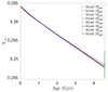 |
Fig. 2. Evolution of the surface helium mass fraction as a function of age for the models of Table 1. The green crosses indicate the surface helium abundance inferred from helioseismology by Basu & Antia (1995). |
In Table 2, we provide the same constraints for models implementing an asymptotic formulation of the combined effect of shear instability, meridional circulation and magnetic Tayler instability. The classical formulation of Spruit (2002) had been put forward in Eggenberger et al. (2022a) as a potential explanation for the lithium depletion as a result of the shear in the solar radiative envelope being reduced to an appropriate value. This formulation is, however, shown to lead to a too high depletion of beryllium at the age of the Sun compared to the observations (Amarsi et al. 2024). This is further confirmed from the supplementary materials of Eggenberger et al. (2022a) (see their Fig. S3), which show that their mixing coefficient of chemicals goes as low as 0.4 R⊙, exhibiting a relatively flat behaviour.
However, as Buldgen et al. (2024a) mention and multiple works (Cantiello et al. 2014; Deheuvels et al. 2020) note, another key issue of the classical formalism of the Tayler-Spruit dynamo is its inability to reproduce the internal rotation of solar-like subgiants and red giants. Revision of the formalism by Fuller et al. (2019) and an ad hoc recalibration of the efficiency of the coefficient for the dissipation of the magnetic fields (CT) in Eggenberger et al. (2022b) have been suggested to increase the efficiency of the angular momentum transport after the main sequence. In what follows, the impact of such revisions on the solar properties is studied in detail. We start by providing the global parameters of the solar models in Table 2. The exponents in Eq. (2) are varied following Eggenberger et al. (2022b), n = 3 being linked with Fuller et al. (2019), where Eggenberger et al. (2022b) assumed two modifications of CT to marginally improve the agreement with post-main sequence rotation, namely CT = 1 or 0.125, n = 1, and CT = 256 being their suggested recalibration. From Table 2, we can already grasp the main problem of models including a recalibrated version of the magnetic Tayler instability, namely that their behaviour is that of a standard solar model. Indeed, the main impact of these modified formalisms is to lock the allowed shear below a given threshold, provided by Eq. (12) in Eggenberger et al. (2022b). Therefore, when using the recalibrated formalisms with the same horizontal turbulence efficiency, the allowed threshold is so low that no mixing of chemicals occurs during the main sequence.
The evolution of the photospheric lithium and beryllium abundances is illustrated in Fig. 3 for the various models, including the asymptotic treatment of macroscopic mixing by shear, circulation, and magnetic instabilities. A clear pattern again emerges from this analysis, namely that the need for a very efficient angular momentum transport to reproduce the core rotation of red giants pushes the models with this implementation of macroscopic transport to behave like standard models and show no depletion of light elements.
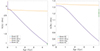 |
Fig. 3. Light element depletion as a function of age for solar models. Left panel: Lithium depletion as a function of age for models including an asymptotic treatment of the magnetic instabilities. Right panel: Beryllium depletion as a function of age for models including an asymptotic treatment of the magnetic instabilities. In both panels, models using the revised treatment of magnetic instabilities, namely Model D |


We made further attempts, including overshooting and an opacity increase replacing the BCZ at the helioseismic value, to attempt to find a regime where such models could simultaneously reproduce the lithium and beryllium depletion. The results for these attempts are illustrated in Fig. 4. Again, even if we reduce the efficiency of the mixing and increase the lithium depletion during the PMS as a result of envelope overshooting, the mixing induced by the combined effects of magnetic instabilities, shear, and circulation goes too deep and leads to a too high depletion of beryllium at the age of the Sun. This confirms the trends that Amarsi et al. (2024) observe on a larger set of models. We will come back to the physical implications of these results in Sect. 3.
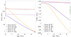 |
Fig. 4. Light element depletion as a function of age for solar models. Left panel: Lithium depletion as a function of age for models including an asymptotic treatment of the magnetic instabilities coupled with overshooting or opacity increase. Right panel: Beryllium depletion as a function of age for models including an asymptotic treatment of the magnetic instabilities coupled with overshooting or opacity increase. In both panels, models using the revised treatment of magnetic instabilities, namely Model OP D |


As mentioned above, the position of the BCZ matters significantly for the calibration of macroscopic transport. Indeed, the overall mixing efficiency will likely be overestimated in AAG21 models that show a significant mismatch in their position of the BCZ. A thinner envelope leads to lower temperatures at the BCZ and thus requires a more efficient mixing to deplete lithium and beryllium. In previous works (e.g. Buldgen et al. 2024a), we discuss the impact of using overshooting or an opacity increase to replace the BCZ position in models including macroscopic mixing. As shown in Buldgen et al. (2023), including adiabatic overshooting to correct the BCZ in solar models leads to a too high depletion of lithium in young solar twins. We therefore chose here to focus on the effect of an opacity increase in our models. We summarize in Table 3 the main properties of these models. As can be seen, our evolutionary models are tailored to reproduce the BCZ position and are in good agreement with the helium abundance inferred from helioseismology. The required opacity increase was modelled in the same way as in Buldgen et al. (2024a), with an amplitude of about 14% close to the BCZ. As we can see from the naming convention of the models, the efficiency of the mixing for a given n is approximately half of what is required in Table 1. This is a direct result of the change in position of the BCZ as a function of time.
Global parameters of the solar evolutionary models reproducing both lithium and beryllium, and BCZ position.
In Fig. 5, we illustrate the lithium and beryllium depletion as a function of time for the models of Table 3. By allowing ourselves to modify both parameters of Eq. (1), reproducing both constraints becomes quite straightforward, and we see that agreeing with the beryllium abundance at the solar age also leads to a much narrower evolution of lithium as a function of time. From the observed trends in the behaviour of the mixing coefficient, it appears that allowed values of n range between 3 and 6, with the lower values leading to a slightly too high depletion of beryllium and the highest ones to almost no depletion at all. This is in line with the calibrated values found in A-type stars with n = 3 or 4 (Richer et al. 2000; Richard et al. 2001; Michaud et al. 2005). Further extending such analyses to solar-like stars observed with the Kepler mission for which high-quality asteroseismic data are available might provide more insight into the underlying physical process responsible for lithium depletion as well as further test its link with angular momentum transport mechanisms.
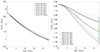 |
Fig. 5. Light element depletion as a function of age for solar models. Left panel: Lithium depletion as a function of time for the models of Table 3, including an opacity increase at the BCZ. Right panel: Beryllium depletion as a function of time for the models of Table 3. The green crosses indicate the observed values at the current solar age. |
2.2. Constraints on macroscopic transport efficiency
In Fig. 6, we illustrate the evolution of the surface helium mass fraction as a function of time and the metallicity profile of our models, reproducing both lithium and beryllium photospheric abundances and the BCZ position through an opacity increase. The first striking feature of these models is the very narrow range of initial and final helium abundance they exhibit. A slight trend is observed with more pronounced coefficients (higher values of n) leading to slightly lower final helium values as a result of the shallower mixing regions that allow for a larger impact of settling on the evolution. This is a direct result of the calibration of the mixing using beryllium that essentially controls the efficiency required during the main sequence. This implies that a relatively narrow range of final and initial helium abundances is allowed when macroscopic mixing is included, allowing us to refine previous estimates of protosolar helium based on standard solar models (Serenelli & Basu 2010).
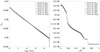 |
Fig. 6. Left panel: Surface helium mass fraction evolution as a function of time for our models including macroscopic transport and opacity modifications. Right panel: Metallicity profile as a function of normalized radius for the our models including macroscopic transport and opacity modifications. |
A second important feature of the models is the similarities in the metallicity profile close to the BCZ. Essentially, the presence of efficient transport in these layers leads to the metals being efficiently mixed down to 0.6 R⊙. Some form of differentiation between the various efficiencies appears below these layers, where the effects of settling may still be felt. Nevertheless, this spread remains small and the same conclusion can be drawn looking at the central metallicity values. These results have strong implications for neutrino fluxes, as we will see in Sect. 2.3, and are a natural result of models including macroscopic mixing.
2.3. Impact on helioseismic results and neutrino fluxes
We illustrate in Fig. 7 the sound speed profile for our models, including macroscopic mixing at the BCZ and an opacity increase in its vicinity to replace its position at the helioseismic value. As can be seen, the usual deviation at the BCZ has been completely erased by the combination of the opacity increase and the macroscopic mixing. Some deviations nevertheless remain in the radiative layers and in the core. Such effects have been seen in previous studies (see e.g. Buldgen et al. 2023, 2024a) and can be attributed to the lowering of the core metallicity that results from the effects of macroscopic mixing on the calibration. As mentioned above, the effects are similar to helium and thus a lower initial metallicity is found for models including macroscopic mixing compared to standard solar models that only consider the effects of settling. It is no surprise that the localized increase in opacity we implemented, following Buldgen et al. (2024a), does not correct the lower layers. We stress again that the opacity modification implemented here is not based on a physical process; we merely implemented a Gaussian-like increase of about 14% in the vicinity of the iron peak around log T = 6.35, similarly to previous extended calibration experiments (Ayukov & Baturin 2017; Kunitomo & Guillot 2021). It is likely that some of the effects currently being studied (Pain & Gilleron 2020; Pradhan 2024; Pradhan et al. 2024) would also impact higher temperature regions in the solar models. Therefore, Fig. 7 mostly illustrates how the BCZ region can be easily corrected and how models including macroscopic transport show very similar properties in their deeper radiative layers, which was already hinted at from looking at Fig. 6.
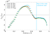 |
Fig. 7. Relative squared adiabatic sound speed differences between the Sun and models including macroscopic mixing and an opacity increase at the BCZ reproducing both Be and Li photospheric abundances. |
The situation is similar for neutrino fluxes regarding the comparative behaviours of the models that are provided in Table 4. Given their similar chemical evolution and initial chemical composition resulting from the solar calibration, they have quite similar central conditions, and therefore neutrino fluxes. However, in this case, macroscopic mixing leads to much lower fluxes for ϕ(Be), ϕ(B), and ϕ(CNO), and therefore to a stark disagreement with observed values if we focus on the Borexino results. The situation is not so problematic if one considers the values that the work of Orebi Gann et al. (2021) provides, based on multiple experiments. This is also in agreement with what we find in Buldgen et al. (2024a) for models using the abundances of Magg et al. (2022). This issue is more pronounced for the AAG21 models, as they start from a lower initial value due to their intrinsically lower metallicity. It remains to be seen whether other processes such as planetary formation (Kunitomo et al. 2022) might compensate for the lowering of the central metallicity or whether other effects may come into play. Indeed, planetary formation through the evolution of the metallicity of the accreted matter from the protosolar disk may significantly impact the central metallicity at the current solar age and lead to an increase of about 5%. Further tests with the latest nuclear reaction rates (Acharya et al. 2024) and the effects of dynamical electronic screening may need to be investigated. It should also be mentioned that potential opacity revisions (Bailey et al. 2015; Pain & Gilleron 2020; Pradhan 2024; Pradhan et al. 2024) may also extend to higher temperatures and affect the initial conditions of solar calibrations and thus the predicted neutrino fluxes of solar models. In addition, a steeper macroscopic transport coefficient also seems to slightly reduce the impact on neutrino fluxes, although by a very small amount.
Neutrino fluxes of the evolutionary models.
3. Link with magnetic Tayler instability
As discussed above, the magnetic Tayler instability is a potential candidate, alongside fossil magnetic fields (Gough & McIntyre 1998) and internal gravity waves (Charbonnel & Talon 2005; Pinçon et al. 2016), for explaining the current solar rotation profile. While some debate existed in the literature regarding its potential occurrence in hydrodynamical simulations (Zahn et al. 2007), recent works by Petitdemange et al. (2023) show that it was actually present in their simulations. Revision of the work of Spruit (2002) was carried out by Fuller et al. (2019) to explain the slow rotation of red giants and core-helium-burning stars.
From Figs. 3 and 4, we can see that there seems to be an intrinsic problem with the macroscopic transport provided by the asymptotic depiction of rotation and the magnetic Tayler instability. In the “classical” case of the initial Spruit (2002) formulation, the obtained beryllium depletion was too high. This is a direct result of the functional expression of the transport coefficient that goes as deep as 0.4 R⊙ and only has a slow decreasing trend. Indeed, Eggenberger et al. (2022a) show that its efficiency could be reproduced in CLES models using n = 1.3 in the Proffitt & Michaud (1991) formulation. The reason for this efficiency is linked with the allowed shear by the magnetic Tayler instability. Even if the rotation profile appears to be quite flat, the instability is considered to be active only after a given level of shear is reached (see Spruit 2002, for a discussion), meaning that it undergoes some sort of limit cycle that still allows for some mixing of chemicals at the BCZ, where mean molecular weight gradients are formed over time as a result of microscopic diffusion and the envelope slows down as a result of the magnetic braking of the surface.
The main issue with this formulation of the magnetic Tayler instabilities is that it leads to a too low efficiency of the angular momentum transport on the subgiant and red giant branch and is therefore unable to reproduce the asteroseismic constraints for subgiants (Deheuvels et al. 2014, 2020) and red giants (Cantiello et al. 2014). This has led to the derivation of a new formulation by Fuller et al. (2019) and an ad hoc calibration of the efficiency of the magnetic field dissipation in Eggenberger et al. (2022b). Both formulations provide a similar agreement on the red giant branch but fail to reproduce the trend observed in core rotations at the transition between the subgiants and red giants. It is also unclear whether these formulations would agree with recent inferences of the internal rotation of subgiants in Buldgen et al. (2024b). There is also currently no clear justification as to why the instability would switch from the behaviour that Spruit (2002) describe to that of Fuller et al. (2019) at the end of the main sequence.
Regarding the transport of chemical elements, we are either left with a too efficient mixing and large depletion of lithium and beryllium in the standard formulation of the magnetic Tayler instability or no depletion at all in the case of the more efficient formalisms used when studying red giants and subgiants. The remaining question is whether an in-between regime could be derived and whether some free parameters can be tweaked in the equations to ensure a higher depletion of lithium in the new formalisms and a steep decrease of the transport coefficients, allowing the observed beryllium depletion to be simultaneously reproduced.
Turning to the transport equations used in stellar evolutionary models, the only free parameter that can be tweaked is the efficiency of the horizontal turbulence, noted Dh, intervening in both the transport by shear instability and meridional circulation. The transport of chemicals by both these processes is modelled as diffusive, using the following expressions in Eggenberger et al. (2022a).
The diffusive transport of chemicals by rotation is given by the expression
 (3)
(3)
with Deff the transport by the meridional circulation and DX the transport by shear. For the meridional circulation, Deff is defined as
 (4)
(4)
with Dh the horizontal turbulence coefficient and U(r) the velocity of the meridional circulation. Both Dh and U(r) are related through some analytical prescriptions from Zahn (1992), Maeder (2003), and Mathis et al. (2004) that we recall below.
 (5)
(5)
 (6)
(6)
 (7)
(7)
with U(r) and V(r) the vertical and horizontal components of the velocity of the meridional circulation,  the average angular velocity over latitude at a given radius, and
  , while ch, A and β are constants.
Regarding the shear instability, we followed the prescription of Talon & Zahn (1997):
 (8)
(8)
with Dh the horizontal turbulence coefficient, Ric the critical Richardson number, dW/dz = r sin θ(dΩ/dr) the shear rate, K the thermal diffusivity, and Nμ and NT the chemical and thermal contributions to the Brunt-Väisälä frequency.
From a direct comparison between the asymptotic coefficients, we note that the transport coefficient of chemical elements in the revised magnetic instability formalism is about 104 times smaller than the one from the original formulation. This explains why such models behave essentially as standard solar models from a chemical point of view. The key point is that, as noted by Maeder & Meynet (2004), the magnetic Tayler instability itself does not transport a lot of chemicals, and indeed the observed depletion of lithium and beryllium is due to the effect of shear and meridional circulation, as regulated by the magnetic instability to the critical value of shear above which the magnetic Tayler instability operates. It is thus natural that a more efficient magnetic instability leads to a lower degree of shear and thus a lower overall mixing. The remaining question is whether an arbitrary increase in Dh may compensate for this, keeping in mind that intrinsic treatments of the transport of chemicals by rotation might slightly alter the observed trends (Dumont et al. 2021).
First, we can comment on the required increase. An increase of four orders of magnitude already casts doubt on the reliability of the magnetic Tayler instability being considered responsible for the lithium and beryllium depletion in the Sun. Indeed, the horizontal turbulence as derived from the above expressions may lead to values of one or two orders of magnitude at most (see e.g. Nandal et al. 2024, for an application to massive stars). Nevertheless, one could be under the impression that increasing Dh would be the solution, due to the fact that a direct increase in Dh increases DX in Eq. (8) and thus the mixing by the shear instability which could remain localized. However, the increase in Dh would also increase the efficiency of the transport by the meridional circulation. Indeed, in each of the expressions, we see that
 (9)
(9)
with n ≥ 1. This is also in line with Chaboyer & Zahn (1992) and Eqs. (4.37) and (4.38) in Maeder & Zahn (1998). In other words, Deff would increase under both the effect of the increase in Dh and the reduced shear induced by the efficient transport by the magnetic instability, implying that α ≪ 1. Therefore, such an increased transport by the meridional circulation would imply mixing chemicals down to temperatures high enough to lead to the efficient combustion of beryllium.
In essence, the meridional circulation naturally becomes more efficient if the horizontal turbulence is increased, meaning that simultaneous reproduction of both lithium and beryllium may not be achieved by modifying Dh. In other words, the magnetic Tayler instability, in its current implementation or calibration to reproduce observational data, cannot be linked with the depletion of the light elements in the Sun. This is due to its intrinsic inefficient transport of chemicals, leaving other magnetic instabilities (e.g. Jouve et al. 2020; Griffiths et al. 2022; Meduri et al. 2024 when talking about magnetic instabilities), improved depictions of the magnetic Tayler instability (e.g. Petitdemange et al. 2023, 2024) taking into account additional hydrodynamical effects, or other physical mechanisms (Charbonnel & Talon 2005; Pinçon et al. 2016) as remaining candidates. It is, however, worth noting that the light-element depletion in the Charbonnel & Talon (2005) approach was due to the shear-layer oscillation and not the transport by the gravity waves themselves. In practice, this requires further investigation into the actual impact of the solar tachocline and its potential link with the observed lithium and beryllium depletion.
Regarding the magnetic Tayler instability, its eligibility as an angular momentum transport candidate in the Sun is not affected by the conclusions of our analysis, but would require a measurement of the rotation of the deep solar core using gravity modes (Appourchaux et al. 2010; Leibacher et al. 2023) in order to be confirmed beyond doubt, as well as further theoretical developments beyond calibrations of its efficiency to explain the observed trends in asteroseismic inferences. It is also worth mentioning that there is no guarantee that the current picture drawn from asteroseismic inferences requires a unique solution. For example, the presence of a convective core during extended periods of evolution may also influence the presence of magnetic fields inside the star and thus the angular momentum transport in the interior and consequently the observed light-element depletion. In the context of actual measurements of large radial fields (Li et al. 2022, 2023; Hatt et al. 2024), incompatible with the magnetic Tayler instability, it might be worth considering the possibility of multiple explanations or other angular momentum transport candidates.
4. Conclusion
In this paper, we investigate in detail the required properties of macroscopic mixing at the base of the solar convective envelope to simultaneously reproduce the observed lithium (Wang et al. 2021) and beryllium (Amarsi et al. 2024) photospheric abundances. We used solar-calibrated models, including both a simple parametric coefficient for macroscopic transport from Proffitt & Michaud (1991) and an asymptotic formulation based on models including angular momentum transport (Eggenberger et al. 2022a). We also investigate the impact of replacing the base of the convective envelope at the helioseismic value on the inferred efficiency of macroscopic transport. We find that not taking into account the current position of the BCZ may lead to an overestimation of the transport by a factor of two and that the observed lithium and beryllium abundances imply an efficient transport with a relatively short extent, in line with what has been found in more massive stars (Richer et al. 2000). This behaviour is impossible to reproduce with the current implementations of the effects of shear, meridional circulation, and magnetic Tayler instability, which intrinsically lead to an efficient mixing down to higher temperatures. We investigated the possibility of using revised prescriptions of these effects based on the current issues with angular momentum transport after the main sequence and find that such models present almost no mixing, as a result of the reduced shear allowed by the revised magnetic Tayler instabilities (Fuller et al. 2019; Eggenberger et al. 2022b). Our findings thus cast doubt on the ability to link the observed light-element depletion to the combined effects of shear, circulation, and magnetic Tayler instability, as suggested in Eggenberger et al. (2022a).
Our final calibration, using a power law of density, as in Proffitt & Michaud (1991), leads to values of n in Eq. (1) of between 3 and 6, the efficiency of the transport at the BCZ varying depending on this exact value but being of about 6000 cm2/s for moderate values of n that are in line with the values found for AMFM stars (Richer et al. 2000).
Further analyses on solar-like stars observed by Kepler might provide additional insights as to the underlying physical mechanism behind the light-element depletion. In this respect, the Kepler LEGACY sample (Lund et al. 2017; Silva Aguirre et al. 2017) might provide the perfect test bed, as helium abundance in the envelope of some stars may be inferred from asteroseismic data and correlated with lithium and beryllium depletion (when these are available). Indeed, Verma et al. (2017) show the need to introduce additional turbulent mixing (Verma & Silva Aguirre 2019). The availability of surface or even internal rotation for some of these stars makes them prime targets for furthering our understanding of the missing dynamical processes in our current generation of stellar models. Due to their importance as tracers of mixing, and the key role of lithium in primordial nucleosynthesis models, further extension of our analysis to low-metallicity regimes and globular clusters would also provide additional tests of the prescriptions we use for the Sun in a more global context of the theory of stellar structure and evolution. In this respect, the role of the PLATO mission (Rauer et al. 2024) in providing additional high-quality asteroseismic targets for high-quality spectroscopic follow-up will be crucial. Such stars would allow us to define the basic requirements for the underlying processes leading to the observed light-element depletion and their potential link to the efficient angular momentum transport processes acting in the solar and stellar interiors.
Acknowledgments
We thank the referee for their careful reading of the manuscript. GB acknowledges fundings from the Fonds National de la Recherche Scientifique (FNRS) as a postdoctoral researcher. AMA gratefully acknowledges support from the Swedish Research Council (VR 2020-03940) and from the Crafoord Foundation via the Royal Swedish Academy of Sciences (CR 2024-0015). We acknowledge support by the ISSI team “Probing the core of the Sun and the stars” (ID 423) led by Thierry Appourchaux.
References
- Acharya, B., Aliotta, M., Balantekin, A. B., et al. 2024, ArXiv e-prints [arXiv:2405.06470] [Google Scholar]
- Amarsi, A. M., Ogneva, D., Buldgen, G., et al. 2024, A&A, 690, A128 [NASA ADS] [CrossRef] [EDP Sciences] [Google Scholar]
- Anders, E., & Grevesse, N. 1989, Geochim. Cosmochim. Acta, 53, 197 [Google Scholar]
- Appel, S., Bagdasarian, Z., Basilico, D., et al. 2022, Phys. Rev. Lett., 129, 252701 [NASA ADS] [CrossRef] [Google Scholar]
- Appourchaux, T., Belkacem, K., Broomhall, A. M., et al. 2010, A&ARv, 18, 197 [Google Scholar]
- Asplund, M. 2004, A&A, 417, 769 [NASA ADS] [CrossRef] [EDP Sciences] [Google Scholar]
- Asplund, M., Grevesse, N., Sauval, A. J., & Scott, P. 2009, ARA&A, 47, 481 [NASA ADS] [CrossRef] [Google Scholar]
- Asplund, M., Amarsi, A. M., & Grevesse, N. 2021, A&A, 653, A141 [NASA ADS] [CrossRef] [EDP Sciences] [Google Scholar]
- Ayukov, S. V., & Baturin, V. A. 2017, Astron. Rep., 61, 901 [NASA ADS] [CrossRef] [Google Scholar]
- Bailey, J. E., Nagayama, T., Loisel, G. P., et al. 2015, Nature, 517, 3 [Google Scholar]
- Balachandran, S. C., & Bell, R. A. 1998, Nature, 392, 791 [NASA ADS] [CrossRef] [Google Scholar]
- Baraffe, I., Pratt, J., Goffrey, T., et al. 2017, ApJ, 845, L6 [Google Scholar]
- Basilico, D., Bellini, G., Benziger, J., et al. 2023, Phys. Rev. D, 108, 102005 [NASA ADS] [CrossRef] [Google Scholar]
- Basinger, C., Pinsonneault, M., Bastelberger, S. T., Gaudi, B. S., & Domagal-Goldman, S. D. 2024, MNRAS, 534, 2968 [NASA ADS] [CrossRef] [Google Scholar]
- Basu, S., & Antia, H. M. 1995, MNRAS, 276, 1402 [NASA ADS] [Google Scholar]
- Basu, S., & Antia, H. M. 1997, MNRAS, 287, 189 [NASA ADS] [CrossRef] [Google Scholar]
- Basu, S., Chaplin, W. J., Elsworth, Y., New, R., & Serenelli, A. M. 2009, ApJ, 699, 1403 [NASA ADS] [CrossRef] [Google Scholar]
- Baturin, V. A., Gorshkov, A. B., & Ayukov, S. V. 2006, Astron. Rep., 50, 1001 [NASA ADS] [CrossRef] [Google Scholar]
- Baturin, V. A., Ayukov, S. V., Gryaznov, V. K., et al. 2013, ASP Conf. Ser., 479, 11 [NASA ADS] [Google Scholar]
- Boesgaard, A. M. 1988, Vistas Astron., 31, 167 [NASA ADS] [CrossRef] [Google Scholar]
- Boesgaard, A. M. 2023, ApJ, 943, 40 [NASA ADS] [CrossRef] [Google Scholar]
- Boesgaard, A. M., & Deliyannis, C. P. 2024, ApJ, 972, 136 [NASA ADS] [CrossRef] [Google Scholar]
- Boesgaard, A. M., & Krugler Hollek, J. 2009, ApJ, 691, 1412 [NASA ADS] [CrossRef] [Google Scholar]
- Boesgaard, A. M., Deliyannis, C. P., Lum, M. G., & Chontos, A. 2022, ArXiv e-prints [arXiv:2209.15158] [Google Scholar]
- Borexino Collaboration (Agostini, M., et al.) 2018, Nature, 562, 505 [CrossRef] [Google Scholar]
- Borexino Collaboration (Agostini, M., et al.) 2020, Nature, 587, 577 [NASA ADS] [CrossRef] [Google Scholar]
- Brun, A. S., Antia, H. M., Chitre, S. M., & Zahn, J.-P. 2002, A&A, 391, 725 [NASA ADS] [CrossRef] [EDP Sciences] [Google Scholar]
- Buldgen, G., Eggenberger, P., Noels, A., et al. 2023, A&A, 669, L9 [NASA ADS] [CrossRef] [EDP Sciences] [Google Scholar]
- Buldgen, G., Noels, A., Scuflaire, R., et al. 2024a, A&A, 686, A108 [NASA ADS] [CrossRef] [EDP Sciences] [Google Scholar]
- Buldgen, G., Fellay, L., Bétrisey, J., et al. 2024b, A&A, 689, A307 [NASA ADS] [CrossRef] [EDP Sciences] [Google Scholar]
- Cantiello, M., Mankovich, C., Bildsten, L., Christensen-Dalsgaard, J., & Paxton, B. 2014, ApJ, 788, 93 [Google Scholar]
- Carlos, M., Nissen, P. E., & Meléndez, J. 2016, A&A, 587, A100 [NASA ADS] [CrossRef] [EDP Sciences] [Google Scholar]
- Carlos, M., Meléndez, J., Spina, L., et al. 2019, MNRAS, 485, 4052 [Google Scholar]
- Chaboyer, B. 1998, IAU Symp., 185, 25 [NASA ADS] [Google Scholar]
- Chaboyer, B., & Zahn, J. P. 1992, A&A, 253, 173 [NASA ADS] [Google Scholar]
- Charbonneau, P., Barnes, G., & MacGregor, K. B. 2000, IAU Joint Discussion, 24, 14 [NASA ADS] [Google Scholar]
- Charbonnel, C., & Talon, S. 2005, Science, 309, 2189 [Google Scholar]
- Chmielewski, Y., Brault, J. W., & Mueller, E. A. 1975, A&A, 42, 37 [NASA ADS] [Google Scholar]
- Christensen-Dalsgaard, J. 2021, Liv. Rev. Sol. Phys., 18, 2 [NASA ADS] [CrossRef] [Google Scholar]
- Christensen-Dalsgaard, J., Gough, D. O., & Thompson, M. J. 1991, ApJ, 378, 413 [NASA ADS] [CrossRef] [Google Scholar]
- Christensen-Dalsgaard, J., Dappen, W., Ajukov, S. V., et al. 1996, Science, 272, 1286 [Google Scholar]
- Christensen-Dalsgaard, J., Gough, D. O., & Knudstrup, E. 2018, MNRAS, 477, 3845 [CrossRef] [Google Scholar]
- Deal, M., & Martins, C. J. A. P. 2021, A&A, 653, A48 [NASA ADS] [CrossRef] [EDP Sciences] [Google Scholar]
- Deal, M., Richard, O., & Vauclair, S. 2021, A&A, 646, A160 [NASA ADS] [CrossRef] [EDP Sciences] [Google Scholar]
- Deheuvels, S., Doğan, G., Goupil, M. J., et al. 2014, A&A, 564, A27 [NASA ADS] [CrossRef] [EDP Sciences] [Google Scholar]
- Deheuvels, S., Ballot, J., Eggenberger, P., et al. 2020, A&A, 641, A117 [EDP Sciences] [Google Scholar]
- Dumont, T., Palacios, A., Charbonnel, C., et al. 2021, A&A, 646, A48 [EDP Sciences] [Google Scholar]
- Eggenberger, P., Buldgen, G., Salmon, S. J. A. J., et al. 2022a, Nat. Astron., 6, 788 [NASA ADS] [CrossRef] [Google Scholar]
- Eggenberger, P., Moyano, F. D., & den Hartogh, J. W. 2022b, A&A, 664, L16 [NASA ADS] [CrossRef] [EDP Sciences] [Google Scholar]
- Ferguson, J. W., Alexander, D. R., Allard, F., et al. 2005, ApJ, 623, 585 [Google Scholar]
- Fuller, J., Piro, A. L., & Jermyn, A. S. 2019, MNRAS, 485, 3661 [NASA ADS] [Google Scholar]
- Gough, D. O., & McIntyre, M. E. 1998, Nature, 394, 755 [Google Scholar]
- Grevesse, N., & Sauval, A. J. 1998, Space Sci. Rev., 85, 161 [Google Scholar]
- Griffiths, A., Eggenberger, P., Meynet, G., Moyano, F., & Aloy, M.-A. 2022, A&A, 665, A147 [NASA ADS] [CrossRef] [EDP Sciences] [Google Scholar]
- Gryaznov, V. K., Ayukov, S. V., Baturin, V. A., et al. 2004, AIP Conf. Ser., 731, 147 [NASA ADS] [CrossRef] [Google Scholar]
- Hatt, E. J., Ong, J. M. J., Nielsen, M. B., et al. 2024, MNRAS, 534, 1060 [NASA ADS] [CrossRef] [Google Scholar]
- Iglesias, C. A., & Rogers, F. J. 1996, ApJ, 464, 943 [NASA ADS] [CrossRef] [Google Scholar]
- Jørgensen, A. C. S., & Weiss, A. 2018, MNRAS, 481, 4389 [Google Scholar]
- Jouve, L., Lignières, F., & Gaurat, M. 2020, A&A, 641, A13 [EDP Sciences] [Google Scholar]
- Kunitomo, M., & Guillot, T. 2021, A&A, 655, A51 [NASA ADS] [CrossRef] [EDP Sciences] [Google Scholar]
- Kunitomo, M., Guillot, T., & Buldgen, G. 2022, A&A, 667, L2 [NASA ADS] [CrossRef] [EDP Sciences] [Google Scholar]
- Leibacher, J., Appourchaux, T., Buldgen, G., et al. 2023, BAAS, 55, 235 [NASA ADS] [Google Scholar]
- Li, G., Deheuvels, S., Ballot, J., & Lignières, F. 2022, Nature, 610, 43 [NASA ADS] [CrossRef] [Google Scholar]
- Li, G., Deheuvels, S., Li, T., Ballot, J., & Lignières, F. 2023, A&A, 680, A26 [NASA ADS] [CrossRef] [EDP Sciences] [Google Scholar]
- Lodders, K. 2021, Space Sci. Rev., 217, 44 [NASA ADS] [CrossRef] [Google Scholar]
- Lund, M. N., Silva Aguirre, V., Davies, G. R., et al. 2017, ApJ, 835, 172 [Google Scholar]
- Lyubimkov, L. S. 2016, Astrophysics, 59, 411 [NASA ADS] [CrossRef] [Google Scholar]
- Lyubimkov, L. S. 2018, Astrophysics, 61, 262 [NASA ADS] [CrossRef] [Google Scholar]
- Maeder, A. 2003, A&A, 399, 263 [NASA ADS] [CrossRef] [EDP Sciences] [Google Scholar]
- Maeder, A., & Meynet, G. 2004, A&A, 422, 225 [NASA ADS] [CrossRef] [EDP Sciences] [Google Scholar]
- Maeder, A., & Zahn, J.-P. 1998, A&A, 334, 1000 [NASA ADS] [Google Scholar]
- Magg, E., Bergemann, M., Serenelli, A., et al. 2022, A&A, 661, A140 [NASA ADS] [CrossRef] [EDP Sciences] [Google Scholar]
- Mamajek, E. E., Prsa, A., Torres, G., et al. 2015, ArXiv e-prints [arXiv:1510.07674] [Google Scholar]
- Mathis, S., Palacios, A., & Zahn, J. P. 2004, A&A, 425, 243 [NASA ADS] [CrossRef] [EDP Sciences] [Google Scholar]
- Meduri, D. G., Jouve, L., & Lignières, F. 2024, A&A, 683, A12 [NASA ADS] [CrossRef] [EDP Sciences] [Google Scholar]
- Michaud, G., Richer, J., & Richard, O. 2005, ApJ, 623, 442 [NASA ADS] [CrossRef] [Google Scholar]
- Nandal, D., Meynet, G., Ekström, S., et al. 2024, A&A, 684, A169 [NASA ADS] [CrossRef] [EDP Sciences] [Google Scholar]
- Orebi Gann, G. D., Zuber, K., Bemmerer, D., & Serenelli, A. 2021, Annu. Rev. Nucl. Part. Sci., 71, 491 [CrossRef] [Google Scholar]
- Pain, J.-C., & Gilleron, F. 2020, High Energy Density Physics, 34, 100745 [NASA ADS] [CrossRef] [Google Scholar]
- Paquette, C., Pelletier, C., Fontaine, G., & Michaud, G. 1986, ApJS, 61, 177 [Google Scholar]
- Petitdemange, L., Marcotte, F., & Gissinger, C. 2023, Science, 379, 300 [NASA ADS] [CrossRef] [Google Scholar]
- Petitdemange, L., Marcotte, F., Gissinger, C., & Daniel, F. 2024, A&A, 681, A75 [NASA ADS] [CrossRef] [EDP Sciences] [Google Scholar]
- Pinçon, C., Belkacem, K., & Goupil, M. J. 2016, A&A, 588, A122 [NASA ADS] [CrossRef] [EDP Sciences] [Google Scholar]
- Pinsonneault, M. 1997, ARA&A, 35, 557 [NASA ADS] [CrossRef] [Google Scholar]
- Pinsonneault, M. H., Kawaler, S. D., Sofia, S., & Demarque, P. 1989, ApJ, 338, 424 [Google Scholar]
- Pradhan, A. K. 2024, J. Phys. B At. Mol. Phys., 57, 125003 [NASA ADS] [CrossRef] [Google Scholar]
- Pradhan, A. K., Nahar, S. N., & Eissner, W. 2024, J. Phys. B At. Mol. Phys., 57, 125001 [NASA ADS] [CrossRef] [Google Scholar]
- Proffitt, C. R., & Michaud, G. 1991, ApJ, 380, 238 [Google Scholar]
- Rauer, H., Aerts, C., Cabrera, J., et al. 2024, ArXiv e-prints [arXiv:2406.05447] [Google Scholar]
- Richard, O., Vauclair, S., Charbonnel, C., & Dziembowski, W. A. 1996, A&A, 312, 1000 [NASA ADS] [Google Scholar]
- Richard, O., Michaud, G., & Richer, J. 2001, ApJ, 558, 377 [Google Scholar]
- Richer, J., Michaud, G., & Turcotte, S. 2000, ApJ, 529, 338 [Google Scholar]
- Salaris, M., & Cassisi, S. 2017, Roy. Soc. Open Sci., 4, 170192 [Google Scholar]
- Schou, J., Antia, H. M., Basu, S., et al. 1998, ApJ, 505, 390 [Google Scholar]
- Scuflaire, R., Théado, S., Montalbán, J., et al. 2008, Ap&SS, 316, 83 [Google Scholar]
- Serenelli, A. M., & Basu, S. 2010, ApJ, 719, 865 [NASA ADS] [CrossRef] [Google Scholar]
- Silva Aguirre, V., Lund, M. N., Antia, H. M., et al. 2017, ApJ, 835, 173 [Google Scholar]
- Spruit, H. C. 2002, A&A, 381, 923 [CrossRef] [EDP Sciences] [Google Scholar]
- Swenson, F. J., & Faulkner, J. 1991, in Challenges to Theories of the Structure of Moderate-Mass Stars, eds. D. Gough, & J. Toomre, 388, 345 [NASA ADS] [CrossRef] [Google Scholar]
- Talon, S., & Zahn, J. P. 1997, A&A, 317, 749 [NASA ADS] [Google Scholar]
- Thévenin, F., Oreshina, A. V., Baturin, V. A., et al. 2017, A&A, 598, A64 [NASA ADS] [CrossRef] [EDP Sciences] [Google Scholar]
- Thoul, A. A., Bahcall, J. N., & Loeb, A. 1994, ApJ, 421, 828 [Google Scholar]
- Turcotte, S., Richer, J., Michaud, G., Iglesias, C. A., & Rogers, F. J. 1998, ApJ, 504, 539 [Google Scholar]
- Verma, K., & Silva Aguirre, V. 2019, MNRAS, 489, 1850 [NASA ADS] [CrossRef] [Google Scholar]
- Verma, K., Raodeo, K., Antia, H. M., et al. 2017, ApJ, 837, 47 [NASA ADS] [CrossRef] [Google Scholar]
- Vinyoles, N., Serenelli, A. M., Villante, F. L., et al. 2017, ApJ, 835, 202 [NASA ADS] [CrossRef] [Google Scholar]
- Wang, E. X., Nordlander, T., Asplund, M., et al. 2021, MNRAS, 500, 2159 [Google Scholar]
- Zahn, J. P. 1992, A&A, 265, 115 [NASA ADS] [Google Scholar]
- Zahn, J. P., Brun, A. S., & Mathis, S. 2007, A&A, 474, 145 [NASA ADS] [CrossRef] [EDP Sciences] [Google Scholar]
All Tables
Global parameters of the solar evolutionary models reproducing both lithium and beryllium, and BCZ position.
All Figures
|
Fig. 1. Depletion of light element as a function of age for solar models. Left panel: Lithium depletion as a function of age for the solar models in Table 1. Right panel: Beryllium depletion as a function of age for the solar models in Table 1. The green crosses indicate the observed values of lithium (Wang et al. 2021) and beryllium (Amarsi et al. 2024). The duration of the PMS phase in our models is 40 Myr and leads to a significant depletion of lithium and a moderate depletion of beryllium, which are unfortunately barely visible. |
| In the text | |
|
Fig. 2. Evolution of the surface helium mass fraction as a function of age for the models of Table 1. The green crosses indicate the surface helium abundance inferred from helioseismology by Basu & Antia (1995). |
| In the text | |
|
Fig. 3. Light element depletion as a function of age for solar models. Left panel: Lithium depletion as a function of age for models including an asymptotic treatment of the magnetic instabilities. Right panel: Beryllium depletion as a function of age for models including an asymptotic treatment of the magnetic instabilities. In both panels, models using the revised treatment of magnetic instabilities, namely Model D |
| In the text | |
|
Fig. 4. Light element depletion as a function of age for solar models. Left panel: Lithium depletion as a function of age for models including an asymptotic treatment of the magnetic instabilities coupled with overshooting or opacity increase. Right panel: Beryllium depletion as a function of age for models including an asymptotic treatment of the magnetic instabilities coupled with overshooting or opacity increase. In both panels, models using the revised treatment of magnetic instabilities, namely Model OP D |
| In the text | |
|
Fig. 5. Light element depletion as a function of age for solar models. Left panel: Lithium depletion as a function of time for the models of Table 3, including an opacity increase at the BCZ. Right panel: Beryllium depletion as a function of time for the models of Table 3. The green crosses indicate the observed values at the current solar age. |
| In the text | |
|
Fig. 6. Left panel: Surface helium mass fraction evolution as a function of time for our models including macroscopic transport and opacity modifications. Right panel: Metallicity profile as a function of normalized radius for the our models including macroscopic transport and opacity modifications. |
| In the text | |
|
Fig. 7. Relative squared adiabatic sound speed differences between the Sun and models including macroscopic mixing and an opacity increase at the BCZ reproducing both Be and Li photospheric abundances. |
| In the text | |
Current usage metrics show cumulative count of Article Views (full-text article views including HTML views, PDF and ePub downloads, according to the available data) and Abstracts Views on Vision4Press platform.
Data correspond to usage on the plateform after 2015. The current usage metrics is available 48-96 hours after online publication and is updated daily on week days.
Initial download of the metrics may take a while.