| Issue |
A&A
Volume 681, January 2024
|
|
|---|---|---|
| Article Number | A60 | |
| Number of page(s) | 14 | |
| Section | The Sun and the Heliosphere | |
| DOI | https://doi.org/10.1051/0004-6361/202245638 | |
| Published online | 11 January 2024 | |
Impulsively generated waves in two-fluid plasma in the solar chromosphere: Heating and generation of plasma outflows
1
Institute of Physics, University of M. Curie-Skłodowska, Pl. M. Curie-Skłodowskiej 1, 20-031 Lublin, Poland
2
Department of Physics, University of Helsinki, Helsinki, Finland
3
Shenzhen Key Laboratory of Numerical Prediction for Space Storm, Institute of Space Science and Applied Technology, Harbin Institute of Technology, 518055 Shenzhen, PR China
e-mail: kuzma@hit.edu.cn
4
Key Laboratory of Solar Activity and Space Weather, National Space Science Center, Chinese Academy of Sciences, 100190 Beijing, PR China
Received:
7
December
2022
Accepted:
21
October
2023
Context. We present new insights into impulsively generated Alfvén and magneto-acoustic waves in the partially ionized two-fluid plasma of the solar atmosphere and their contribution to chromospheric heating and plasma outflows.
Aims. Our study attempts to elucidate the mechanisms responsible for chromospheric heating and excitation of plasma outflows that may contribute to the generation of the solar wind in the upper atmospheric layers. The main aim of this work is to investigate the impulsively generated waves by taking into account two-fluid effects. These effects may alter the wave propagation leading to attenuation and collisional plasma heating.
Methods. The two-fluid equations were solved by the JOint ANalytical Numerical Approach (JOANNA) code in a 2.5-dimensional (2.5D) framework to simulate the dynamics of the solar atmosphere. Here, electrons + ions (protons) and neutrals (hydrogen atoms) are treated as separate fluids, which are coupled via ion-neutral collisions. The latter acts as a dissipation mechanism for the energy carried by the waves in two-fluid plasma and may ultimately lead to the frictional heating of the partially ionized plasma. The waves in two-fluid plasma, which are launched from the top of the photosphere, are excited by perturbations induced by localized Gaussian pulses in the horizontal components of the ion and neutral velocities.
Results. In the middle and upper chromosphere, a substantial fraction of the energy carried by large amplitude waves in the two-fluid plasma is dissipated in ion-neutral collisions, resulting in the thermalization of wave energy and generation of plasma outflows. We find that coupled Alfvén and magneto-acoustic waves are more effective in heating the chromosphere than magneto-acoustic waves.
Conclusions. Large-amplitude waves in the two-fluid plasma may be responsible for heating the chromosphere. The net flow of ions is directed outward, leading to plasma outflows in the lower solar corona, which may contribute to the solar wind at higher altitudes The primary source of wave energy dissipation in the current paradigm comes from collisions between ions and neutrals.
Key words: Sun: abundances / Sun: chromosphere / Sun: activity / Sun: atmosphere / solar wind / Sun: corona
© The Authors 2024
 Open Access article, published by EDP Sciences, under the terms of the Creative Commons Attribution License (https://creativecommons.org/licenses/by/4.0), which permits unrestricted use, distribution, and reproduction in any medium, provided the original work is properly cited.
This article is published in open access under the Subscribe to Open model. Subscribe to A&A to support open access publication.
1. Introduction
As a result of the relatively low temperatures the photosphere and chromosphere remain only partially ionized (Zaqarashvili et al. 2011). The degree of ionization in the photosphere is about 10−4, and the ratio of the number of ions to neutrals increases with height in the chromosphere (Khomenko et al. 2014). Therefore, studies of these atmospheric layers using analytical and numerical approaches should take into account the presence of neutrals. Zaqarashvili et al. (2011) was the first to demonstrate that the single-fluid technique may be inadequate for partially ionized plasma. They contrasted the outcomes of single-fluid (describing the evolution of ions only) and two-fluid (for ions + electrons and neutrals) models and concluded that the investigated single-fluid technique failed for time scales comparable to ion-neutral collision time-scale in a partially-ionized plasma. Recent studies have also revealed the importance of two-fluid models for a much wider range of solar phenomena. For instance, Martínez-Gómez et al. (2018) studied nonlinear Alfvén waves in partially-ionized plasma using a multi-fluid model that accounts for the impact of elastic collisions between all plasma species. The conditions they investigated were similar to those of a quiescent solar prominence and the authors summarise that the effects of non-linearity are stronger for standing waves than for propagating waves. The two-fluid numerical modeling of the coronal rain blob in the isothermal stratified solar atmosphere was discussed by Martínez-Gómez et al. (2022). They inferred that ion-neutral decoupling causes an increase in the drift velocity and temperature that can result in increased emission from the plasma present at the edge of the coronal rain. Song et al. (2023) modeled the formation of the transition region using a two-fluid approach and reported on the essential structural characteristic of the transition region.
Since the chromosphere has a higher mass density than the solar corona, it radiates energy more rapidly than the corona; thus, an extra heating mechanism is required to compensate for this loss. The energy inputs from the lower layers of the solar atmosphere are insufficient to compensate for this loss. Various possible mechanisms behind the local heating of the chromosphere were briefly reviewed in Narain & Ulmschneider (1991, 1996), and references therein. Hollweg (1985) considered turbulence as the main dissipation mechanism and proposed that Alfvén waves (Alfvén 1942) are the prime candidates for energy transport. Convective instabilities in plasma usually propagate in the form of magneto-hydrodynamic (MHD) waves. These waves include fast, and slow magneto-acoustic waves (hereafter MAWs) and Alfvén waves (Musielak 1992). The damping of MHD waves by ion-neutral collisions and the thermalization of wave energy may also play an important role in chromospheric heating (e.g., Erdélyi & James 2004; Niedziela et al. 2021; Pelekhata et al. 2021; Tu & Song 2013; Song & Vasyliūnas 2011). Kuźma et al. (2020) reported that substantial damping caused by ion-neutral collisions allows nonlinear Alfvén waves to efficiently heat the chromosphere. However, such waves are not able to account for the heat losses in the solar atmosphere plasma because of their small amplitudes. Recently, Zhang et al. (2021a) studied acoustic wave propagation and energy deposition while accounting for ionization and recombination as well as ion-neutral collisions. They showed that the energy deposition in partially ionized plasma may be underestimated due to ionization and recombination. On the other hand, Niedziela et al. (2021) and Pelekhata et al. (2021) performed parametric studies and showed that impulsively generated large-amplitude Alfvén and MAWs heat the chromosphere through ion-neutral collisions and generate plasma outflows in the low solar corona.
Large amplitude waves may also turn into shocks that may heat the solar atmosphere. For instance, Orta et al. (2003) concluded that MHD shocks could be a plausible mechanism for coronal heating and solar wind acceleration in open magnetic field line regions of strongly magnetized plasma. Fawzy et al. (2002) conducted a study taking the shock formation as a means of dissipation of the wave energy. They determined the energy balance between the most notable chromospheric radiative losses and the dissipated wave energy as a function of the height in the solar atmosphere. In contrast, Wójcik et al. (2020) examined the wave heating by replacing the shock formation with ion-neutral collisions. Here the authors concluded an agreement with the semi-empirical model of Avrett & Loeser (2008).
The aim of this paper is to extend the models of Niedziela et al. (2021) and Pelekhata et al. (2021) by considering linearly coupled Alfvén and MAWs in two-fluid plasma and to study how they contribute to the heating of the chromosphere and to the generation of the plasma outflows. Niedziela et al. (2021) showed the heating of the chromospheric plasma by the two-fluid MAWs and neutral acoustic waves by ion-neutral collisions. These waves were excited by perturbations in the vertical component of the ion and neutral velocities (i.e., Viy, Vny), while keeping the transversal component of the background magnetic field zero (i.e., Bz = 0 Gs). We note that the 1D models used by the authors prevented the propagation of internal gravity waves. Pelekhata et al. (2021) reported that large amplitude Alfvén waves can contribute to plasma heating in the chromosphere by initially injecting the perturbations in the transversal component of ion and neutral velocities (i.e., Viz, Vnz). In addition, Niedziela et al. (2021) and Pelekhata et al. (2021) excited the waves by small amplitude Gaussian pulses in the vertical and transverse components of velocities, respectively. In the present study, the linearly coupled Alfvén and MAWs are generated by launching the Gaussian pulse in a 2.5D system in the horizontal component of the ion and neutral velocities (i.e., Vix, Vnx).
This paper is organized as follows. Section 2 consists of a set of the governing two-fluid equations describing the dynamics of the plasma in the solar atmosphere. Section 3 describes the setup of our numerical simulations. The numerical results are presented and discussed in Sect. 4. An overview and conclusions are given in Sect. 5.
2. Model of the solar atmosphere
2.1. Two-fluid equations
The plasma in the lower layers of the solar atmosphere is a self-consistent system, meaning that each particle simultaneously affects the other particle with its electric and magnetic field. Since the spatial scales of interest are large compared to the mean free path, following the trajectories of each particle would be a daunting task. However, the majority of the plasma phenomena can be explained by the fluid models where the identity of each particle is ignored and treated as a continuum, that is, as a fluid (Roy & Pandey 2002). As aforementioned, it is consequently crucial to consider the behavior of neutral particles along with ions in these atmospheric layers. Therefore, the gravitationally stratified and magnetically confined solar atmosphere is represented by a two-fluid numerical model. We treat ions + electrons and neutrals as two distinct interacting fluids and each fluid has its own characteristics in terms of flow velocity, mass density, and gas pressure (e.g., Zaqarashvili et al. 2011; Maneva et al. 2017; Popescu Braileanu et al. 2019, and references therein). Other species are not considered here for the sake of simplicity. We assume that ions comprise protons and neutrals are hydrogen atoms. Factors such as recombination, ionization, the influence of electrons on ions, charge exchange, heat conduction, and radiative losses are not considered in this model (e.g., Murawski et al. 2022). The two-fluid model in this paper is based on the following set of equations:
(a) mass conservation equations:
(b) momentum equations:

(c) energy equations:
![$$ \begin{aligned}&\frac{\partial E_{\rm i}}{\partial t} + \nabla \cdot \left[\left(E_{\rm i}+ p_{\mathrm{ie}}+ \frac{{\boldsymbol{B}}^2}{2\mu }\right){\boldsymbol{V}}_{\rm i}-\frac{{\boldsymbol{B}}}{\mu }(V_{\rm i}\cdot \boldsymbol{B})\right] = (\varrho _{\rm i}{\boldsymbol{g}} + {\boldsymbol{S}}_{\rm m})\cdot {\boldsymbol{V}}_{\rm i} + Q_{\rm i}, \end{aligned} $$](/articles/aa/full_html/2024/01/aa45638-22/aa45638-22-eq5.gif)
![$$ \begin{aligned}&\frac{\partial E_{\rm n}}{\partial t} + \nabla \cdot [(E_{\rm n} + p_{\rm n}){\boldsymbol{V}}_{\rm n}] = (\varrho _{\rm n}\boldsymbol{g} - {\boldsymbol{S}}_{\rm m})\cdot {\boldsymbol{V}}_{\rm n} + Q_{\rm n}, \end{aligned} $$](/articles/aa/full_html/2024/01/aa45638-22/aa45638-22-eq6.gif)
with energy densities given as
Induction and solenoidal constraints supplement the aforementioned equations, expressed as:
In Eqs. (1)–(8), subscripts i and n denote ion and neutral components, 𝜚i, 𝜚n are mass densities, Ei, En energy densities, Ti, Tn temperatures, pie, pn denote the ion+electron and neutral gas pressures (Eq. (13)), while Vi, Vn represent ion and neutral velocities. The magnetic field and magnetic permeability are denoted respectively by B and μ and I stands for the identity matrix. The gravitational acceleration (g) points toward the negative y-axis with magnitude 274.78 m s−2, γ is the ratio of specific heat under constant pressure to its constant volume counterpart, here taken as 5/3. Other symbols have their standard meaning. Collisional momentum, Sm, and energy exchange terms, Qi, Qn are defined as (Oliver et al. 2016; Meier & Shumlak 2012):
Here, vin is ion-neutral collision frequency defined as (Braginskii 1965; Ballester et al. 2018)
with mi = mHμi and mn = mHμn being respectively the mass of ions and neutrals, taken here equal to the hydrogen mass (mH). The symbols μi = 1, μn = 1 are respectively the mean masses of ions and neutrals. The collision cross section (σin) here is taken as 1.4 × 10⁻¹⁹ m2 (Vranjes & Krstic 2013; Chapman & Cowling 1970). Ion and neutral temperatures are specified by the ideal gas laws:
Here, kB is the Boltzmann constant. Unlike MHD models, two-fluid models separately simulate ions + electrons and neutrals, allowing the assumptions of quasi-neutrality, small Larmor radius, and small Debye length to be dropped. The two-fluid equations accurately describe the chromosphere and low corona, which is a region of attention in the present model, but they have limitations in illustrating the photosphere (Khomenko et al. 2014).
2.2. Magneto-hydrostatic equilibrium of the solar atmosphere
We initially (i.e., at t = 0 s) assume that the plasma in the solar atmosphere is in magneto-hydrostatic equilibrium. Magneto-hydrostatic equilibrium is the state for still fluids (Vi = 0) in which the radially outward pressure gradient force is balanced by the inward gravitational force. In mathematical terms, it can be described as:
The above expression can be obtained from Eqs. (3) and (4) by setting Vi = Vn = 0 and B = 0. Here, the hydro-static gas pressure and mass densities are expressed respectively as (e.g., Kuźma et al. 2017)
where Λie, n = kBT/μie, ng are ion and neutral pressure scale-heights that are specified by T(y) taken from the semi-empirical model of Avrett & Loeser (2008). We note that the pressure scale height is the distance in the isothermal atmosphere (not considered here) at which pressure the decreases by e times. The equilibrium pressures of the ions and neutrals at the reference height are denoted by p0ie, n. The reference height is taken at y = yr = 50 Mm with p0n = 0.05 Pa and p0ie = 0.1 Pa. Figure 1 illustrates the temperature (a) and mass density (b) profiles of ions (dashed) and neutrals (dotted) with the height adapted from the model of Avrett & Loeser (2008). We note that T(y) attains its minimum at y ≈ 0.6 Mm. At y = 2.1 Mm, a sharp rise in the temperature can be seen, reaching a magnitude of about 106 K at y ≈ 10 Mm as expected in the solar corona (not shown). The mass-density profiles are then obtained using Eqs. (15) and (16). In the photosphere and in the low chromosphere, 𝜚i (dashed) is lower than 𝜚n (dotted) attributed to its low-temperature region. However, for y ≥ 1.5 Mm, especially in the transition region (i.e., y ≈ 2.1 Mm), 𝜚n starts to drop considerably. This clearly demonstrates that the ionization degree depends on the height above the photosphere.
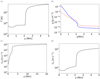 |
Fig. 1. Vertical profiles of equilibrium temperature (a) (Avrett & Loeser 2008), the mass density of ions (dotted) and neutrals (dashed) (b), bulk Alfvén speed (c), and sound speed (d) in the two-fluid model of the solar atmosphere for initial magneto-hydrostatic equilibrium configuration. Initially (i.e., at t = 0 s), the temperature of ions (Ti) and neutrals (Tn) are considered to be equal, but later on, this assumption is relaxed, and Ti, Tn are permitted to vary. |
The variation of bulk Alfvén speed, CA (c), and sound speed, CS, (d) with height is shown in Fig. 1. These quantities are specified, respectively, as:
The bulk Alfvén speed in the lower chromosphere (y ≈ 1 Mm) attains a value of about 10 km s−1. It increases until the transition region, where it experiences a sharp rise and then settles to an approximately steady value. The main reason behind this sudden increase is the fall of the plasma mass density as demonstrated in Fig. 1b. The variation of the sound speed CS with height is shown in Fig. 1d, which follows the trend of T(y) at the transition region. In the photosphere (0 ≤ y ≤ 0.5 Mm), CS attains its lowest value of approximately 10 km s−1.
The overlying magnetic field configuration is expected to impact the propagation and properties of Alfvén and MAWs (Bogdan et al. 2003). A current-free and thus force-free (i.e., (∇×B)×B/μ = 0) magnetic field is implemented on the aforementioned hydro-static equilibrium. The hydro-static equilibrium as given by Eqs. (14) and (16) is overlaid by a uniform and unidirectional magnetic field, namely, B = [0, By, Bz], with the vertical component assumed to be fixed to By = 10 Gs. This value of By corresponds to the magnetic field strength in the quiet sun (see, for instance, Fig. 1 in Shelyag et al. 2012). In this study, we investigate and compare two cases of the Bz, namely (a) Bz = 0 Gs and (b) Bz = 2 Gs. The rationale for selecting Bz = 2 Gs stems from the fact that the typical strength of B in the corona between 1.05 and 1.35 solar radii lies within the range of 1−4 Gs (Yang et al. 2020). Because we are considering a uniform magnetic field configuration in our model, B remains the same in the lower layers of the solar atmosphere as well, namely in the photosphere and chromosphere. As a result, the magnetic field specified above is within the bounds of observational findings and it is physically justified.
2.3. Impulsive perturbations
To excite Alfvén and MAWs, the Gaussian pulses are initially (i.e., at t = 0 s) launched in the horizontal components of the ion, and neutral velocities These Gaussian pulses are specified as follows:

Here, A, w, and y0 respectively denote the amplitude of pulse, width, and launching height. We note that the physical nature of natural disturbances, on the other hand, is far more intricate than the reliance indicated by Eq. (19). However, this rather simplistic approach allows us to understand the physics behind this mechanism.
We consider A = 6 km s−1, w = 0.25 Mm, and y0 = 0.5 Mm unless otherwise stated. Notably, this value of w is consistent with the spatial scale of solar granules which have a typical diameter range of 200−1000 km (Cloutman 1980). The chosen value of y0 = 0.5 Mm corresponds to the top of the photosphere. In the present model, A is much larger than the amplitude of the horizontal flow in a solar granule (e.g., Stein & Nordlund 1998) but may occasionally take place there as a result of magnetic reconnection. Therefore, the values picked above are scientifically justified and within the bounds of the physical phenomena that exist in the solar atmosphere.
Large-scale dynamical changes that can transmit kinetic energy, such as buffeting caused by granular motion in the photosphere, blast waves caused by flares in the high atmosphere, shocks as a result of magnetic reconnection, and so on, continuously disturbing the atmospheric magnetic field. Here, the Gaussian pulse of Eq. (19) mimics a sudden buffeting of magnetic field lines by granular cells. When a perturbation is applied to the magnetic field, it affects the plasma present in the surrounding region. The interaction between the perturbed magnetic field and the plasma leads to the propagation of waves. These waves carry energy and information higher up in the solar atmosphere, causing oscillations and disturbances in the magnetic field and the plasma itself.
3. Simulation setup
To investigate the role of linearly coupled Alfvén and MAWs in heating the chromosphere and the higher layers of the solar atmosphere, we have to rely on numerical simulation and modeling. The JOANNA code, developed by Wójcik et al. (2020) which is based on the higher-order Godunov-type method (e.g., Wójcik et al. 2018), is implemented to solve the two-fluid equations (Eqs. (1)–(6)). We set the Courant-Friedrichs-Lewy number equal to 0.9 (Courant et al. 1928), which is allowed by the use of accurate third-order Runge-Kutta method (Durran 2010) of discretization of temporary derivatives, which strongly preserves the stability here. We note that the divergence of the B is not naturally achieved by the solution of the two-fluid equations. Therefore, the magnetic monopoles must be cleaned using the method from Dedner et al. (2002).
The simulation region is specified as −2.56 Mm ≤ x ≤ 2.56 Mm and 0 ≤ y ≤ 40 Mm. Along the y-direction, the distance between 0 and 5.12 Mm is divided uniformly into 2048 cells. Therefore, the size of each numerical cell in this region is Δy = 2.5 km. On the other hand, above 5.12 Mm, the grid is stretched and covered by 32 cells resulting in the size of each cell being about Δy ≈ 1090 km at the top boundary. A stretched grid acts like an absorbent, which damps or absorbs the incoming signal and minimizes polluting reflections from the top boundary. Along the x-direction, the grid is covered by the 2048 cells resulting in the size of each cell Δx = 2.5 km. At t = 0 s, we keep all plasma quantities set to their equilibrium values at the bottom and top boundaries, as indicated by Eqs. (14) and (15). The left-and-right sides of the simulation box are specified with the open boundary conditions, which are realized by copying the information from the nearby physical cells into the boundary cells. The total time duration of running the numerical simulation is 3000 s. We note that in this article we use the Cartesian coordinate system, where [x, y, z] stands respectively for the horizontal, vertical, and transversal components.
4. Numerical results
4.1. Numerical tests
Factors such as magnetic field configuration, plasma density, temperature gradients, and collisional processes all impact wave propagation and their evolution in the solar atmosphere. All such factors can result in phenomena like wave reflection, refraction, mode conversion, and energy dissipation (Roberts 1981; Theurer et al. 1997; Morton et al. 2023). However understanding the exact mechanism of wave propagation, coupling, and collisional dissipation necessitates a thorough analysis of the underlying physics, which includes the intricate interaction of numerous processes. It entails examining the wave equations, studying the relevant plasma parameters, and taking into account the effects of collisions and other interactions. Therefore, due to the intricate nature of these processes and their inter-dependencies, the very subject of our investigation, namely, the process of ion and neutral wave propagation, coupling, and collisional energy dissipation, is, in fact, very subtle. Therefore we first address numerical errors in our system. It can be done by performing numerical tests for Bz = 2 Gs since this case takes both Alfvén and MAWs into account. As a result of the discretization of equations on a mesh of finite resolution, we expect some physical perturbations that appear mainly due to numerical errors. To make sure these perturbations have a negligible influence on our main results of interest, we ran the code without launching the Gaussian pulse (i.e., A = 0 in Eq. (19)) and let the system evolve in time without any external disturbances.
Generated numerical noise is shown by the time-distance plots in Fig. 2. The signals in both panels are the result of the numerical approximations and correspond to Alfvén and MAWs. The vertical component of the ion velocity, Viy, is shown in Fig. 2a. It may be noted that Max|Viy|≈0.075 km s−1 occurs above the transition region (y ≈ 2.1 Mm). This value is quite small, however, in comparison to the sound speed in this region (Fig. 1d). The dark red and blue bands are most prominent in the initial 500 s, but such bands damp strongly with time. In the region of interest (0.5 < y < 2 Mm), the magnitude of Viy is negligible.
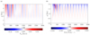 |
Fig. 2. Time-distance plot for Viy (a) and relative perturbation of ion temperature δTi(x = 0, y, t)/T(y) = (Ti(x = 0, y, t)−T(y))/T(y) (b) in the case of no pulse (i.e., A = 0 in Eq. (19)) for Bz = 2 Gs. Here T(y) is adopted from the model of Avrett & Loeser (2008; Fig. 1a). |
The time-distance plot for relative perturbed temperature (i.e., δTi(x = 0, y, t)/T(y) = Ti(x = 0, y, t)−T(y)/T(y)) is shown in Fig. 2b. Here, Ti(x = 0, y, t) denotes the temperature of ions, and T(y) is taken from the model of Avrett & Loeser (2008; Fig. 1, panel a). It is clearly evident that Max|δTi(x = 0, y, t)/T(y)| is about 2 × 10⁻³ which takes place at the transition region (i.e., at y ≈ 2.1 Mm), which is a quite low value as compared to T(y). It is worth noting that here red-blue strips leaning toward the y-axis represent the reflection of the waves from the transition region. Such wave reflections are clearly visible at t ≈ 250 s. The main reason behind such reflection is a rapid increase in the sound speed (Fig. 1, panel d). As waves propagate from the chromosphere into the transition region, the steep profile of the sound speed causes changes in the refractive index of the plasma which leads to a change in the wave speed and direction of wave propagation. A detailed study of wave reflection can be found in Sect. 2 of Wentzel (1978).
We conclude that the numerical errors observed in the system for the chosen numerical grid are negligible and decay strongly with time. Thus, the generated numerical noise is small ensuring that the numerical methods and the chosen grid size do not significantly affect the numerical results.
4.2. Impulsively generated waves: A qualitative description
The implemented Gaussian pulses of Eq. (19) result in different waves in the two-fluid plasma depending on the chosen background magnetic field configuration [Bx, By, Bz], in our case [0, 10, 0] Gs and [0, 10, 2] Gs. A detailed description of the linear MHD waves can be found in the book by Roberts (2019). The propagation of waves in two-fluid in the present model is a rather complex phenomenon, however, in this section, we describe some basic properties of MHD waves in a uniform medium.
Let b1 (b1 ≪ B) and v1 denote respectively perturbations in magnetic field and velocity. Note that velocity perturbations are introduced by the Gaussian pulse as indicated in Eq. (19). Case 1 in Fig. 3a represents where the velocity perturbations, that is, v1 = (vx, vy, 0) have longitudinal components, that is, k ⋅ v1 ≠ 0. Here k is the wave vector. Upon linearising the system of MHD equations about the homogeneous equilibrium and applying the Fourier transform. If  and
and  denote the corresponding Fourier counterparts (respectively) to b1 and v1, then we can find the following two important relations. First, there is the relation between
  and
and  , given as
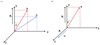 |
Fig. 3. Direction of the velocity perturbations (v1), wave vector (k) for magnetic field B = [0, By, 0] Gs (a) and B = [0, By, Bz] Gs (b). |
Here, ω is the wave angular frequency. The second is the dispersion relation which can be written as:
Here “+” corresponds to the fast, while “−” corresponds to the slow MAWs, and θ is the angle between k and By. Here we will be interested in 0 < θ < π/2. Taking the “+” root, and setting θ = 0, the dispersion relation of Eq. (21) is reduced to ω2 = k2
 which means that the phase speed of fast MAWs is the Alfvén speed in the y direction (that is along the magnetic field). On the other hand, for θ = π/2, the dispersion relation reduces to
  . This implies that fast MAWs are fastest along a direction perpendicular to the magnetic field. Taking the “−” root, when θ = 0, the dispersion relation of Eq. (21) reduces to ω2 = k2
 , which means that along y, slow MAWs travel with tube speed,
  . For θ = π/2, ω = 0, which indicates that slow MAWs cannot travel perpendicularly to the magnetic field direction.
The initial pulses of Eq. (19) introduce the perturbations for Bz = 0, which, in turn, generate fast and slow ion MAWs and neutral acoustic waves as well as internal gravity waves. In the low chromosphere and below it, where plasma-β = 2μp/B2 > 1, (here, p is the plasma pressure and B2/2μ is the magnetic pressure), fast and slow MAWs are strongly coupled. Higher up, where plasma-β < 1, these waves are weakly coupled (Murawski 2002). Since MAWs are compressive and longitudinal in nature (i.e., k ⋅ v1 ≠ 0), we can trace their overall evolution in ions velocity, Vi (Figs. 4 and 5).
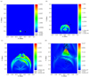 |
Fig. 4. Snapshots of spatial profiles of the total velocity Vi (color map) expressed in the units of km s−1, and velocity vectors (arrows) at t = 0 s (a, launch of Gaussian pulse as mentioned in Eq. (19)), t = 60 s (b), t = 135 s (c), and t = 160 s (d) for initial B = [0, 10, 0] Gs. This configuration will lead to the generation of MAWs. The spatial profile of Vi (color map) here represents the propagation of the MAWs in the chromosphere (0.5 ≤ y ≤ 2 Mm) and in higher layers of the solar atmosphere. The black arrows indicate the direction of the plasma flow. |
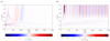 |
Fig. 5. Time-distance plots for Vix (a) and Viy (b) corresponding to MAWs for B = [0, 10, 0] Gs. These plots correspond to the slices collected at x = 0 Mm along y in Fig. 4. The blue and red bands in both panels indicate the propagation of waves with time. |
In a similar way, Fig. 3b represents a case of Bz ≠ 0 where perturbations, v1 = (0, 0, vz) is transverse to the wave vector (k). The dispersion relation can be written as:
A similar description of this configuration can also be found in Sect. 2.1 in Battaglia et al. (2021). For the parallel propagation, θ = 0, the dispersion relation of Eq. (22) is reduced to ω2 = k2
 , which means that Alfvén waves travel along the magnetic field with their phase speed equal to CA. When θ = π/2, ω = 0, as a result, Alfvén waves are unable to propagate perpendicular to the magnetic field direction. Since Alfvén waves are in-compressible and transverse in nature (i.e., k ⋅ v1 = 0), we can trace their evolution in Viz (Figs. 6 and 7). We observe that this configuration will lead to the generation of linearly coupled Alfveń and MAWs (e.g., Pandey et al. 2010). Notably, these waves exhibit distinct characteristics, a feature that aligns with the behavior expected in a two-fluid system.
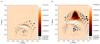 |
Fig. 6. Snapshots of transversal velocity Viz (color map), expressed in the units of km s−1, and velocity vectors (arrows) at t = 100 s (a) and t = 135 s (b) for B = [0, 10, 2] Gs. This configuration leads to the generation of MAWs waves which are coupled to Alfvén waves. Here, the spatial profile of Viz (color map) represents the presence of both Alfvén and MAWs in the chromosphere (0.5 ≤ y ≤ 2 Mm) and in the higher layers of the solar atmosphere. The black arrows indicate the direction of the plasma flow. |
We go on to present numerical results in both cases discussed above (i.e., Bz = 0 Gs and Bz = 2 Gs) to investigate Alfvén and MAWs propagation in the partially ionized solar atmosphere and their effect on plasma heating and outflows.
4.2.1. Magneto-acoustic waves – The case of Bz = 0 Gs
The evaluation of the coupled slow and fast MAWs can be traced in the total ion velocity,  . The snapshots of the spatial profiles of
  overlaid with Vi vectors (arrows) at some notable moments over time are shown in Fig. 4. The initial Gaussian pulse launched at t = 0 s can be seen as a localized perturbation at the top of the photosphere (Fig. 4a). As time progresses, the Gaussian pulse moves, indicating the propagation of MAWs as illustrated in Sect. 4.2. A comparison of the plots at t = 0 s (a) and at t = 160 s (d) clearly manifests how plasma flow initially directed along the horizontal direction (i.e., x) is diverted to the vertical direction (i.e., y).
As the Gaussian pulse spreads further in space, the amplitude of Vi first falls to the value of A = 1.96 km s−1 at t ≈ 60 s (b) and then rises in amplitude to A = 3.15 km s−1 at t ≈ 135 s (c). This increase in amplitude is due to a fall-off background plasma mass density with height (Fig. 1, panel b). Around the same time, the signal approaches the transition region (y ≈ 2.1 Mm) leaving behind the convective instabilities at the launching site (i.e., y = 0.5 Mm). At t ≈ 160 s, the amplitude of the signal is almost doubled from the initial value at t = 0 (e.g., Murawski et al. 2018). Upon passing the transition region, a very steep profile is observed, with a large patch of red color indicating high velocity. This steep wavefront indicates the formation of a shock wave.
Fast and slow MAWs will primarily propagate in the x-and-y directions. Time-distance plots for the MAWs wave Vix (a) and Viy (b) collected at x = 0, are shown in Fig. 5. The red-blue bands in both figures represent the wave’s progression with time. The time-distance plot for Vix sees the max |Vix|≈4 km s−1 at the top of the photosphere which decays in magnitude with time. The time-distance plot for Viy however does not exhibit a similar trend, indicating that the wave energy is propagating mostly vertically. From the time-distance plot for Viy, we conclude that max |Vix|≈8 km s−1 occurs at the top of the chromosphere, which decays in magnitude with time but is not as strong in the case of Vix. The narrow dark red and blue bands near the transition region (y = 2.1 Mm) signify the generation of a fast shock. The presence of a shock in the transition region indicates that the fast MAWs have undergone nonlinear steepening. However, the time interval for which shocks last is very short, which implies that thermal energy is released until this time because it is expected to be primarily generated at shocks by ion-neutral collisions (Zhang et al. 2021b; Snow & Hillier 2021).
As the waves propagate in the system, the evolution of kinetic energy is inevitable. The ion kinetic energy flux due to slow MAWs can be approximated as  , where symbols have their usual meaning. The time-distance plot for kinetic energy flux due to slow MAWs, FE (a), and its associated time averaged profile (b) is shown in Fig. 8. The time-distance plots exhibit one-to-one correspondence with Viy (Fig. 5b), which means that the majority of the MAWs energy flows in the y direction. The kinetic energy flux reaches a maximum value of 106 erg cm−2 s−1 at the top of the photosphere. Note that the presence of a significant kinetic energy flux near the launching site (y = 0.5 Mm) indicates the efficient transfer of energy from the initial perturbation to the surrounding plasma in the form of MAWs. The rapid flow of the energy (for an initial 200 s) is also clear as the MAWs propagate from the photosphere to the transition region where they encounter partial reflection from the transition region. The reason behind such reflection is the sudden rise of CS with height. As the MAWs propagate upward, they encounter regions of higher CS (Fig. 1d) in the chromosphere and transition region. This gradient affects the wave propagation, causing a sharp transition and a downward flow of some of the energy. As the waves propagate further in the system, the kinetic energy flux decreases due to ion-neutral collisions and the spatial spreading of waves.
The time-average profile of the kinetic energy flux of the slow MAWs (Fig. 8b), indicates a sharp rise and the initial peak of the kinetic energy flux at the launching site (i.e., y = 0.5 Mm). This sharp increase in value represents the immediate response to the initial perturbations. The energy flux is high initially due to the concentrated energy carried by the MAWs. As the waves propagate away from the launching site, they encounter ion-neutral collisions which are most effective in the chromosphere giving rise to dissipation mechanisms. As a result, waves spread out and dissipate leading to a falling magnitude of kinetic energy flux (0.5 ≤ y ≤ 1.3 Mm). The subsequent rise from y ≈ 1.3 Mm onward which peaks again at the transition region (y = 2.1 Mm) implies that kinetic energy flux input from the ongoing process compensates MAWs spatial spreading and the dissipation caused by ion-neutral collisions. Beyond the transition region, the energy flux starts decreasing again and reaches approximately a steady. This steady behavior represents a balance between the energy input from the source waves, spatial spreading, and the energy losses due to the dissipation mechanism. The obtained maximum kinetic energy flux values for MAWs (106 erg cm−2 s−1) are about 2 orders of magnitude too small to fulfill radiative losses in the chromosphere, as indicated by Withbroe & Noyes (1977; see their Table 1).
As the MAWs propagate, it perturb the system due to which plasma flows are discernible. The time-distance plots of ion mass flux, Fm(x = 0, y, t) = 𝜚iViy, are illustrated in Figs. 8c, d. These plots provide insight into the up-flows and down-flows of plasma. In the time-distance plot (c), positive mass flux values, indicated by red color, correspond to up-flows. Here, plasma moves away from the photosphere and it is transported to higher layers. On the other hand, negative mass flux values represented by green color imply down-flows, where plasma moves downward toward the photosphere. The alternating red and green bands here correspond to the presence of MAWs. These waves result in regions of up-flows and down-flows of mass flux as they propagate away from the launching site. Initially (at t = 0 s), a dark red patch (Fm(x = 0, y, t)≈2 × 10⁻⁶ g cm−2 s−1) and a dark green patch (Fm(x = 0, y, t)≈ − 2 × 10⁻⁶ g cm−2 s−1) at y = 0.5 Mm indicate, respectively, the presence of strong up-flows and down-flows of plasma due to perturbations at the launching site. Some bands can also be seen leaning toward the y-axis representing the reflection of the MAWs from the transition region (Cally 2022). However, these bands fade away with time strongly suggesting a decay in the amplitude of the waves due to ion-neutral collisions. We note that the observed red and green stripes are limited until y = 1 Mm, which implies that MAWs have a limited vertical extent related to mass flux and their influence is predominantly felt in the lower layer of the chromosphere.
The temporarily averaged profile of mass flux is illustrated in Fig. 8d. In the region, 0 ≤ y ≤ 0.25 Mm, essentially a small value of mass flux represents that there is negligible flow of mass in the middle photosphere. However, in the upper photosphere and chromosphere, the oscillatory behavior of the mass flux suggests the response to MAWs. The magnitude of the mass flux oscillates between −0.7 × 10⁻⁷ g cm−2 s−1 and 0.6 × 10⁻⁷ g cm−2 s−1. For y ≥ 0.75 Mm, the very small steady value of mass flux signifies that no major mass flow in this part of the solar atmosphere. This can be due to the equilibrium condition prevailing in the transition region or the cancellation of the upward and downward mass flux. The value indicated above is approximately ten times less than the value indicated for horizontally averaged total vertical mass flux, ⟨Fm(y, t)⟩, in Wójcik et al. (2019, see their Fig. 5), where the authors reported the result of numerical simulation of the plasma outflows in the context of the origin of solar wind. Thus, the obtained ion mass flux values here are insufficient to fully compensate for solar mass losses in the low corona (Withbroe & Noyes 1977).
4.2.2. Coupled Alfvén and MAWs – The case of Bz = 2 Gs
When Bz is non-zero, the system also allows Alfvén waves to propagate. These waves are linearly coupled to MAWs (e.g., Murawski 2002). Figure 6 shows the snapshots of the typical spatial profiles of the transversal component of ion velocity Viz(x, y) overlaid by the ion velocity vectors (arrows) at t = 100 s (a), and at t = 135 s (b). The observed characteristics in the spatial profile show the perturbation in Viz is non-identically zero, and it is coupled to Vix and Viy, which indicates the presence of Alfvén and MAWs. During the initial phase of evolution (not shown), there are no changes in the spatial profile of Viz(x, y) and the perturbations induced by the Gaussian pulse are still propagating and have not reached the region where notable changes in Viz can be observed. However, at t ≈ 100 s (a), the perturbations begin to propagate in regions of interest, leading to observable changes in the spatial profile of Viz. The perturbation appears well in the form of a red arc moving upward with time. We note that this red arc represents regions of enhanced Viz. At t = 135 s (b), a steepening of the red arc is observed, indicating the development of a steep gradient. Following this region, very light white patches are visible, emphasizing a region of reduced Viz.
The time-distance plots for Vix (a), Viy (b), and Viz (c) collected at x = 0, are shown in Fig. 7. These plots together correspond to the linearly coupled Alfvén-MAWs. We note that the time distance plots for Vix (a) and Viy (b) exhibit characteristics similar to that of Vix and Viy in Fig. 5 (discussed in Sect. 4.2). The time-distance plot for Viz (c) clearly shows oscillations with max |Viz|≈3 km s−1 occurring at the transition region. The reason behind this behavior is the presence of a non-zero Bz component (Bz = 2 Gs) which allows the existence of transverse motions and the generation of Viz which were initially absent for the zero Bz component of the magnetic field.
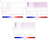 |
Fig. 7. Time-distance plots for Vix (a), Viy (b), and Viz correspond to coupled Alfvén and MAWs for B = [0, 10, 2] Gs. These plots correspond to the slices taken at x = 0 Mm in Fig. 4. The blue and red bands indicate the propagation of the waves. |
The time-distance plots for vertical kinetic energy flux, FE(x = 0, y, t) (a), and the corresponding time-average profile (b) due to slow MAWs are shown in Fig. 9. The similarity to the kinetic energy flux shown in Figs. 8a, b indicates that the additional small z-component could slightly modify the behavior of the waves, but it seems that this change is not significant enough to affect the kinetic energy flux of the MAWs. Similarly, the time-distance plots for vertical mass flux (e) and its corresponding time average profile (f) are shown in Fig. 9 which emphasizes no major noticeable difference as compared to mass flux shown in Figs. 8c, d. This consistent behavior of the kinetic energy and mass fluxes suggests that the primary driver for the energy and mass transport in our simulation is still the magnetic field configuration, particularly the y-component (By).
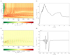 |
Fig. 8. Time-distance plots for kinetic energy flux, FE(x = 0, y, t) (a), and its corresponding vertical profiles averaged over time (b). Time distance plot for total ion vertical mass density flux, Fm(x = 0, y, t) = 𝜚iViy, (c) and its corresponding vertical profiles averaged over time (d). These plots correspond to Fig. 4 and represent the variations of the energy flux (a, b) and mass flux (c, d) due to MAWs. |
The kinetic energy flux due to Alfvén waves is given as  , here CA is the bulk Alfvén speed, and other symbols have their usual meaning. The corresponding time-distance plot is shown in Fig. 9c. The plot manifests characteristics similar to that of the plots for MAWs. The maximum value of FE is 104 erg cm−2 s−1, which is about 100 times less than in the case of the MAWs. This observed difference in magnitude between the energy flux of Alfvén and MAWs is a consequence of the inherent characteristics and energy transport mechanisms of these wave modes. Alfvén waves are transverse in nature and do not involve significant compressional motions in the plasma. Due to their transverse nature and the absence of significant compressional motions, the energy flux associated with Alfvén waves observed here is lower compared to that of MAWs. On the other hand, the energy flux associated with MAWs is primarily carried by the compressional motions of the plasma. These compressional motions may result in relatively large energy flux values.
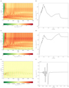 |
Fig. 9. Time-distance plots for kinetic energy fluxes (a, c) and corresponding vertical profiles averaged over time (b, d) for coupled Alfvén and MAWs. The top panels correspond to MAWs while the middle panels correspond to Alfvén waves. Time-distance plot for total ion vertical mass density flux (e) and its corresponding vertical profiles averaged over time (f) for coupled Alfvén magneto-acoustic waves. These plots correspond to Fig. 6. |
4.3. Comparison
The dissipation mechanism for the waves in the present model is ion-neutral collisions. As a result, the excited waves dissipate and transfer some of their energy to the surrounding plasma in the form of thermal energy. Figure 10 demonstrates the time-distance plot for the variations of total collisional heating (Q) due to the first term on RHS of Eqs. (10) and (11) in the case of Bz = 0 (a) and in the case of Bz = 2 Gs (b). The color bar of the time-distance plots provides direct insights into the local energy deposition, and dissipation occurring in different regions due to ion-neutral collisions. In regions, Q attains local maxima where |Vi − Vn| is greater due to the presence of waves. Below y = 0.5 Mm any collisional heating is hardly discernible. In Fig. 10a, the presence of greener patches in the lower chromosphere suggests lower thermal energy deposition. This can be interpreted as the region where the MAWs have relatively weaker energy transfer and dissipation processes. The reduced prominence of greener patches for the chromosphere (Fig. 10, panel b) represents a slightly different distribution of energy transfer and dissipation evolution. Here the presence of coupled Alfvén and MAWs seems to alter the pattern of thermal energy distributions. From this, it can be inferred that coupled Alfvén and MAWs are more efficient and effective in heating the plasma as compared to the MAWs alone.
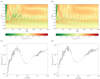 |
Fig. 10. Time-distance plots for thermal energy rate, Q (a, b), and the corresponding vertical time-averaged profile (c, d) in the case of B = [0, 10, 0] Gs (a, c) and B = [0, 10, 2] Gs (b, d). The time distance plots and corresponding time average profile represent the thermal energy rate due to the first term at RHS in Eq. (10). |
The time-averaged profile for Q with y in the case Bz = 0 (c) and Bz = 2 Gs (d) is shown in Fig. 10. Overall both plots exhibit a similar pattern. The sharp rise and peak in Q at y ≈ 0.5 Mm correspond to the location of the initial Gaussian pulse perturbation (Eq. (19)), where the chromospheric plasma witnesses thermal energy push. The high amplitude of the Gaussian pulse leads to a sudden increase in the kinetic energy of the ions and neutrals, resulting in an elevated thermal energy rate. This indicates that the perturbation generates significant thermal energy due to ion-neutral collisions at this location. However, the subsequent decrease in Q and the minima observed at y ≈ 1 Mm can be explained by the dissipation and spatial spreading out of the initially injected energy. The rough linear increase in Q beyond y = 1 Mm can be attributed to the continuous propagation of the perturbation and the transport of energy to higher regions of the atmosphere. The presence of larger amplitude local oscillations in the case Bz = 2 Gs as compared to Bz = 0 indicates the influence of the magnetic field configuration. In the case of Bz = 2, where coupled Alfvén and MAWs are present, the interaction between the magnetic field and the perturbation introduces additional complexity to the dynamics of the system, leading to larger amplitude local oscillations in the thermal energy rate. The local oscillation observed in both cases may be the result of the interference between different wave modes.
5. Summary and discussion
In this paper, we investigate the heating of the partially ionized plasma of the solar atmosphere by Alfvén and MAWs by applying two-fluid numerical simulations. Within the two-fluid models, one set of equations describes the dynamics of ions + electrons and the other neutrals. We considered the impulsively generated waves in the two-fluid plasma that were initially (at t = 0 s) launched by localized Gaussian pulse in the horizontal component of ion and neutral velocities at the top of the photosphere (i.e., y = 0.5 Mm). We investigated their propagation in the 2D for Bz = 0 and 2.5D for Bz = 2 Gs systems. The two fluid equations were solved by using the JOANNA code (Wójcik et al. 2020).
The entire scenario in this paper is linked to energy and mass transport into higher atmospheric layers via plasma outflow. The triggered MAWs and the coupled Alfvén-MAWs thermalize the carried energy due to ion-neutral collisions, contributing to the heating of the plasma in the chromosphere. The overall flow of plasma is directed outward leading to plasma outflow which higher may result in the solar wind. In this paper, we discuss two cases involving the transverse magnetic field, namely, Bz = 0 Gs and Bz = 2 Gs, corresponding to MAWs and coupled Alfvén-MAWs, respectively. Our results showed that coupled Alfvén and MAWs are more effective in heating the chromosphere than the magneto-acoustic wave alone. Our model includes ion-neutral collisions as the only source of wave energy dissipation, which does not generate enough heating to compensate for chromosphere radiative losses as indicated by Withbroe & Noyes (1977; see their Table 1) in either case. However, the plasma outflows, which are correlated to the mass flux, are the same in both cases, that is, MAWs as well as coupled Alfvén-MAWs, as they carry approximately the same amount of mass flux into the solar chromosphere. We concluded that these values of ion mass flux are insufficient to fully compensate for the mass loss caused by the solar wind.
Wave phenomenon and heating of the solar atmosphere is a much more complex phenomenon than described in the present paper. To better describe the solar atmosphere, more accurate simulations are required that take into account additional non-ideal and non-adiabatic effects. Such simulations will be adopted in future studies exploring this topic further.
Acknowledgments
This work was carried out as part of the Space Weather Awareness Training (SWATNet) project, which was funded by the European Union’s Horizon 2020 research and innovation program under grant agreement No. 955620. K.M’s work was done within the framework of the project from the Polish Science Center (NCN) Grant No. 2020/37/B/ST9/00184. The JOANNA code was developed by Dr. Dariusz Wójcik with some contributions from Dr. Luis Kadowaki and Mr. Piotr Wołoszkiewicz. We kindly acknowledge an unknown referee whose comments and suggestions greatly helped in shaping the paper. A part of numerical simulations was run on the LUNAR cluster at the Institute of Mathematics at M. Curie-Skıodowska University in Lublin, Poland. We gratefully acknowledge Poland’s high-performance computing infrastructure PLGrid (HPC Centers: ACK Cyfronet AGH) for providing computer facilities and support within computational grant no. PLG/2022/015868. E.K. acknowledges the Finnish Centre of Excellence in Research of Sustainable Space (Academy of Finland Grant no. 312390, 1352850). We visualize the simulation data using the ViSIt software package (Childs et al. 2012) and Python scripts.
References
- Alfvén, H. 1942, Nature, 150, 405 [Google Scholar]
- Avrett, E. H., & Loeser, R. 2008, ApJS, 175, 229 [Google Scholar]
- Ballester, J. L., Alexeev, I., Collados, M., et al. 2018, Space Sci. Rev., 214, 58 [Google Scholar]
- Battaglia, A. F., Cuissa, J. R. C., Calvo, F., Bossart, A. A., & Steiner, O. 2021, A&A, 649, A121 [NASA ADS] [CrossRef] [EDP Sciences] [Google Scholar]
- Bogdan, T. J., Carlsson, M., Hansteen, V. H., et al. 2003, ApJ, 599, 626 [Google Scholar]
- Braginskii, S. I. 1965, Rev. Plasma Phys., 1, 205 [Google Scholar]
- Cally, P. 2022, Physics, 4, 1050 [NASA ADS] [CrossRef] [Google Scholar]
- Chapman, S., & Cowling, T. G. 1970, The Mathematical Theory of Non-Uniform Gases. An Account of the Kinetic Theory of Viscosity, Thermal Conduction and Diffusion in Gases (Cambridge: Cambridge University Press) [Google Scholar]
- Childs, H., Brugger, E., Whitlock, B., et al. 2012, VisIt: An End-User Tool for Visualizing and Analyzing Very Large Data (Chapman and Hall/CRC), 357 [Google Scholar]
- Cloutman, L. D. 1980, Int. Astron. Union Colloq., 58, 293 [CrossRef] [Google Scholar]
- Courant, R., Friedrichs, K., & Lewy, H. 1928, Math. Annal., 100, 32 [Google Scholar]
- Dedner, A., Kemm, F., Kröner, D., et al. 2002, J. Comput. Phys., 175, 645 [Google Scholar]
- Durran, D. R. 2010, Numerical Methods for Fluid Dynamics (New York: Springer) [CrossRef] [Google Scholar]
- Erdélyi, R., & James, S. P. 2004, A&A, 427, 1055 [NASA ADS] [CrossRef] [EDP Sciences] [Google Scholar]
- Fawzy, D., Rammacher, W., Ulmschneider, P., Musielak, Z. E., & Stȩpień, K. 2002, A&A, 386, 971 [NASA ADS] [CrossRef] [EDP Sciences] [Google Scholar]
- Hollweg, J. V. 1985, in Advances in Space Plasma Physics, eds. W. Grossmann, E. M. Campbell, & B. Buti, 77 [Google Scholar]
- Khomenko, E., Collados, M., Díaz, A., & Vitas, N. 2014, Phys. Plasmas, 21, 092901 [Google Scholar]
- Kuźma, B., Murawski, K., Kayshap, P., et al. 2017, ApJ, 849, 78 [CrossRef] [Google Scholar]
- Kuźma, B., Wójcik, D., Murawski, K., Yuan, D., & Poedts, S. 2020, A&A, 639, A45 [NASA ADS] [CrossRef] [EDP Sciences] [Google Scholar]
- Maneva, Y. G., Alvarez Laguna, A., Lani, A., & Poedts, S. 2017, ApJ, 836, 197 [Google Scholar]
- Martínez-Gómez, D., Soler, R., & Terradas, J. 2018, ApJ, 856, 16 [Google Scholar]
- Martínez-Gómez, D., Oliver, R., Khomenko, E., & Collados, M. 2022, ApJ, 940, L47 [CrossRef] [Google Scholar]
- Meier, E. T., & Shumlak, U. 2012, Phys. Plasmas, 19, 089902 [NASA ADS] [CrossRef] [Google Scholar]
- Morton, R., Sharma, R., Tajfirouze, E., & Miriyala, H. 2023, Rev. Mod. Plasma Phys., 7, 17 [NASA ADS] [CrossRef] [Google Scholar]
- Murawski, K. 2002, Analytical and Numerical Methods for Wave Propagation in Fluid Media (Singapore: World Scientific) [CrossRef] [Google Scholar]
- Murawski, K., Kayshap, P., Srivastava, A. K., et al. 2018, MNRAS, 474, 77 [NASA ADS] [CrossRef] [Google Scholar]
- Murawski, K., Musielak, Z. E., Poedts, S., Srivastava, A. K., & Kadowaki, L. 2022, Ap&SS, 367, 111 [NASA ADS] [CrossRef] [Google Scholar]
- Musielak, Z. 1992, Highlights Astron., 9, 665 [NASA ADS] [CrossRef] [Google Scholar]
- Narain, U., & Ulmschneider, P. 1991, Mechanisms of Chromospheric and Coronal Heating (Heidelberg: Springer-Verlag) [Google Scholar]
- Narain, U., & Ulmschneider, P. 1996, Space Sci. Rev., 75, 453 [Google Scholar]
- Niedziela, R., Murawski, K., & Poedts, S. 2021, A&A, 652, A124 [NASA ADS] [CrossRef] [EDP Sciences] [Google Scholar]
- Oliver, R., Soler, R., Terradas, J., & Zaqarashvili, T. V. 2016, ApJ, 818, 128 [Google Scholar]
- Orta, J. A., Huerta, M. A., & Boynton, G. C. 2003, ApJ, 596, 646 [NASA ADS] [CrossRef] [Google Scholar]
- Pandey, M. K., Prasad, L., & Gariya, S. 2010, Coronal Heating by Coupling of the Magnetosonic and Phase-mixed Alfvén Waves (India: NISCAIR-CSIR) [Google Scholar]
- Pelekhata, M., Murawski, K., & Poedts, S. 2021, A&A, 652, A114 [NASA ADS] [CrossRef] [EDP Sciences] [Google Scholar]
- Popescu Braileanu, B., Lukin, V. S., Khomenko, E., & de Vicente, Á. 2019, A&A, 627, A25 [NASA ADS] [CrossRef] [EDP Sciences] [Google Scholar]
- Roberts, B. 1981, Sol. Phys., 69, 39 [NASA ADS] [CrossRef] [Google Scholar]
- Roberts, B. 2019, MHD Waves in the Solar Atmosphere (Cambridge: Cambridge University Press) [Google Scholar]
- Roy, S., & Pandey, B. P. 2002, Phys. Plasmas, 9, 4052 [NASA ADS] [CrossRef] [Google Scholar]
- Shelyag, S., Mathioudakis, M., & Keenan, F. P. 2012, ApJ, 753, L22 [Google Scholar]
- Snow, B., & Hillier, A. 2021, MNRAS, 506, 1334 [NASA ADS] [CrossRef] [Google Scholar]
- Song, P., & Vasyliūnas, V. M. 2011, J. Geophys. Res. Space Phys., 116, A09104 [NASA ADS] [Google Scholar]
- Song, P., Tu, J., & Wexler, D. B. 2023, ApJ, 948, L4 [NASA ADS] [CrossRef] [Google Scholar]
- Stein, R., & Nordlund, Å. 1998, ApJ, 499, 914 [NASA ADS] [CrossRef] [Google Scholar]
- Theurer, J., Ulmschneider, P., Kalkofen, W., et al. 1997, A&A, 324, 717 [NASA ADS] [Google Scholar]
- Tu, J., & Song, P. 2013, AGU Fall Meeting Abstracts, 2013, SH51A–2088 [Google Scholar]
- Vranjes, J., & Krstic, P. S. 2013, A&A, 554, A22 [NASA ADS] [CrossRef] [EDP Sciences] [Google Scholar]
- Wentzel, D. G. 1978, Sol. Phys., 58, 307 [NASA ADS] [CrossRef] [Google Scholar]
- Withbroe, G. L., & Noyes, R. W. 1977, ARA&A, 15, 363 [Google Scholar]
- Wójcik, D., Murawski, K., & Musielak, Z. E. 2018, MNRAS, 481, 262 [CrossRef] [Google Scholar]
- Wójcik, D., Kuźma, B., Murawski, K., & Srivastava, A. K. 2019, ApJ, 884, 127 [CrossRef] [Google Scholar]
- Wójcik, D., Kuźma, B., Murawski, K., & Musielak, Z. E. 2020, A&A, 635, A28 [NASA ADS] [CrossRef] [EDP Sciences] [Google Scholar]
- Yang, Z., Bethge, C., Tian, H., et al. 2020, Science, 369, 694 [Google Scholar]
- Zaqarashvili, T., Khodachenko, M., & Rucker, H. 2011, A&A, 529, A82 [NASA ADS] [CrossRef] [EDP Sciences] [Google Scholar]
- Zhang, F., Poedts, S., Lani, A., Kuźma, B., & Murawski, K. 2021a, ApJ, 911, 119 [NASA ADS] [CrossRef] [Google Scholar]
- Zhang, F., Poedts, S., Lani, A., Kuźma, B., & Murawski, K. 2021b, EGU General Assembly Conference Abstracts, EGU21–10359 [Google Scholar]
All Figures
|
Fig. 1. Vertical profiles of equilibrium temperature (a) (Avrett & Loeser 2008), the mass density of ions (dotted) and neutrals (dashed) (b), bulk Alfvén speed (c), and sound speed (d) in the two-fluid model of the solar atmosphere for initial magneto-hydrostatic equilibrium configuration. Initially (i.e., at t = 0 s), the temperature of ions (Ti) and neutrals (Tn) are considered to be equal, but later on, this assumption is relaxed, and Ti, Tn are permitted to vary. |
| In the text | |
|
Fig. 2. Time-distance plot for Viy (a) and relative perturbation of ion temperature δTi(x = 0, y, t)/T(y) = (Ti(x = 0, y, t)−T(y))/T(y) (b) in the case of no pulse (i.e., A = 0 in Eq. (19)) for Bz = 2 Gs. Here T(y) is adopted from the model of Avrett & Loeser (2008; Fig. 1a). |
| In the text | |
|
Fig. 3. Direction of the velocity perturbations (v1), wave vector (k) for magnetic field B = [0, By, 0] Gs (a) and B = [0, By, Bz] Gs (b). |
| In the text | |
|
Fig. 4. Snapshots of spatial profiles of the total velocity Vi (color map) expressed in the units of km s−1, and velocity vectors (arrows) at t = 0 s (a, launch of Gaussian pulse as mentioned in Eq. (19)), t = 60 s (b), t = 135 s (c), and t = 160 s (d) for initial B = [0, 10, 0] Gs. This configuration will lead to the generation of MAWs. The spatial profile of Vi (color map) here represents the propagation of the MAWs in the chromosphere (0.5 ≤ y ≤ 2 Mm) and in higher layers of the solar atmosphere. The black arrows indicate the direction of the plasma flow. |
| In the text | |
|
Fig. 5. Time-distance plots for Vix (a) and Viy (b) corresponding to MAWs for B = [0, 10, 0] Gs. These plots correspond to the slices collected at x = 0 Mm along y in Fig. 4. The blue and red bands in both panels indicate the propagation of waves with time. |
| In the text | |
|
Fig. 6. Snapshots of transversal velocity Viz (color map), expressed in the units of km s−1, and velocity vectors (arrows) at t = 100 s (a) and t = 135 s (b) for B = [0, 10, 2] Gs. This configuration leads to the generation of MAWs waves which are coupled to Alfvén waves. Here, the spatial profile of Viz (color map) represents the presence of both Alfvén and MAWs in the chromosphere (0.5 ≤ y ≤ 2 Mm) and in the higher layers of the solar atmosphere. The black arrows indicate the direction of the plasma flow. |
| In the text | |
|
Fig. 7. Time-distance plots for Vix (a), Viy (b), and Viz correspond to coupled Alfvén and MAWs for B = [0, 10, 2] Gs. These plots correspond to the slices taken at x = 0 Mm in Fig. 4. The blue and red bands indicate the propagation of the waves. |
| In the text | |
|
Fig. 8. Time-distance plots for kinetic energy flux, FE(x = 0, y, t) (a), and its corresponding vertical profiles averaged over time (b). Time distance plot for total ion vertical mass density flux, Fm(x = 0, y, t) = 𝜚iViy, (c) and its corresponding vertical profiles averaged over time (d). These plots correspond to Fig. 4 and represent the variations of the energy flux (a, b) and mass flux (c, d) due to MAWs. |
| In the text | |
|
Fig. 9. Time-distance plots for kinetic energy fluxes (a, c) and corresponding vertical profiles averaged over time (b, d) for coupled Alfvén and MAWs. The top panels correspond to MAWs while the middle panels correspond to Alfvén waves. Time-distance plot for total ion vertical mass density flux (e) and its corresponding vertical profiles averaged over time (f) for coupled Alfvén magneto-acoustic waves. These plots correspond to Fig. 6. |
| In the text | |
|
Fig. 10. Time-distance plots for thermal energy rate, Q (a, b), and the corresponding vertical time-averaged profile (c, d) in the case of B = [0, 10, 0] Gs (a, c) and B = [0, 10, 2] Gs (b, d). The time distance plots and corresponding time average profile represent the thermal energy rate due to the first term at RHS in Eq. (10). |
| In the text | |
Current usage metrics show cumulative count of Article Views (full-text article views including HTML views, PDF and ePub downloads, according to the available data) and Abstracts Views on Vision4Press platform.
Data correspond to usage on the plateform after 2015. The current usage metrics is available 48-96 hours after online publication and is updated daily on week days.
Initial download of the metrics may take a while.