© The Authors 2024

1. Introduction

The solar atmosphere can be divided into distinct layers with different physical characteristics, namely: the photosphere, the chromosphere, the transition region, and the corona. The photosphere is considered the conventional surface of the Sun, which spans a height of about 500 km. The chromosphere develops up to a level of about 2100 km and is capped by the corona, which is assumed to extend out into the solar wind over a distance of about 2–3 solar radii. Between the chromosphere and the corona, there is a narrow plasma layer known as the transition region, which is only 100–200 km thick. The temperature variation between these layers, which leads to varying degrees of ionization in the solar atmosphere, is a significant characteristic.

The temperature at the bottom of the photosphere is around 5600 K, gradually falling off with height to a minimum of about 4300 K. This minimum occurs around 100 km above the photosphere. From there, the temperature gradually rises again, first slowly in the low chromosphere, then much faster from the high chromosphere and in the transition region. On average, the temperature in the transition region is 10⁴ − 10⁵ K, abruptly increasing to 1 − 3 × 10⁶ K in the corona. The reason for this temperature increase with height remains a major unknown in heliophysics (Uchida & Kaburaki 1974; Ofman 2010).

The ionization degree is a measure of the number density ratio of particles that have been ionized to the total number of particles. It is influenced directly by the plasma temperature; a lower temperature corresponds to a lower ionization degree. A low ionization degree indicates that the majority of the matter is not ionized, with many atoms retaining their electrons. Due to its extremely high temperature, the solar corona is completely ionized, while the lower and less hot regions of the solar atmosphere are only weakly (the photosphere) and partially (the chromosphere) ionized. In the photosphere, the ionization degree is roughly 10⁻⁴, which means that there is only one ion per about 10⁴ neutral particles. In the chromosphere, the ionization degree increases with height, which motivates and justifies using the multi-fluid model of the solar atmosphere. These observations have been reported by Aschwanden (2005) and Avrett (2003). It should be noted that Brchnelova et al. (2023) shows that even in the almost fully ionized solar corona, the very low abundance of neutrals has a considerable effect on the flow field in the corona.

The recent investigation by Alharbi et al. (2022) shows that the partially ionized plasma can also be divided into two different regions based on the collisional frequency, and this divergence appears around the chromosphere’s base. In the lowest region (the photosphere), the collisional frequency of the charged particles (ions and electrons) is higher than the gyro-frequencies of the charged particles, meaning that the dynamics of the particles are not much affected by the magnetic fields and that the gas dynamics can be described within the framework of a three-fluid plasma model. In this model, the ions, electrons, and neutrals are treated as three separate fluids. In the higher layer (the chromosphere), only the electrons are magnetized. Nevertheless, the strong coupling of the charged particles reduces the working framework to essentially a three-fluid plasma model.

Previously we conducted a study using only a two-fluid model of the solar atmospheric plasma, from which electrons were excluded, and their influence was mimicked by setting the mean mass of the ion+electron gas to 0.5 (Pelekhata et al. 2021). In particular, we studied the effect of Alfvén waves and their coupling with magneto-acoustic waves on the thermalization of the lower solar atmosphere and plasma outflows (Pelekhata et al. 2023). Murawski et al. (2022) investigated the impact of granulation-induced two-fluid waves within the nonideal and nonadiabatic quiet Sun atmosphere. The findings reveal that these waves heat the surrounding medium efficiently and simultaneously generate subtle plasma outflows. While we usually consider only the photosphere and the lower chromosphere, performing studies within a two-fluid framework is reasonable. We did this in an attempt to clarify whether electron pressure contributes to the granulation-generated solar chromosphere heating or whether it is not necessary to particularize our model.

The remainder of this paper is organized as follows: Section 2 presents the simplified three-fluid equations and the background equilibrium model of the solar atmosphere. Section 3 presents the results of the numerical simulations, and Section 4 contains a discussion and summary of the results of the numerical experiments performed and the conclusions that can be drawn from them.

2. Physical model

To simulate the lower atmospheric layers of the Sun, a model of the partially ionized solar atmosphere stratified by a constant gravity was used. The initial setup for the numerical model, including the stratified temperature, is adopted from previous studies (Niedziela et al. 2021; Pelekhata et al. 2021, 2023; Niedziela et al. 2022; Murawski et al. 2022). Specifically, we used the model from Avrett & Loeser (2008) for the initial temperature of ions and neutrals. This study focuses on the quiet Sun region, ensuring that our model accurately represents the temperature stratification observed in this part of the Sun’s atmosphere. The presence of neutral particles in the photosphere and chromosphere, as reported by Khomenko et al. (2014), and recently also by Murawski et al. (2022), necessitates the use of at least a two-fluid plasma model. However, this project applies a simplified three-fluid framework, where a single ion+electron fluid is separated into two distinct fluids, but the electrons are treated as mass-less, and a third fluid describes the dynamics of the neutrals. These fluids interact directly among themselves through ion–neutral, electron–neutral, and electron–ion collisions.

2.1. Simplified three-fluid equations

The simplified three-fluid equations describe the behavior of the species using magnetohydrodynamic-like equations for charges and the Navier–Stokes equations for neutrals. These equations for ions and neutrals can be written as follows:

the continuity equations:

$$\begin{array}{cc}\hfill \frac{\partial {\varrho }_{\mathrm{i}}}{\partial t}+\mathrm{\nabla }·({\varrho }_{\mathrm{i}}{\mathit{V}}_{\mathrm{i}})& =m_{\mathrm{i}}({\mathrm{\Gamma }}_{\mathrm{i}}^{\mathrm{ion}}+{\mathrm{\Gamma }}_{\mathrm{i}}^{\mathrm{rec}}),\hfill \end{array}$$(1)

$$\begin{array}{cc}\hfill \frac{\partial {\varrho }_{\mathrm{n}}}{\partial t}+\mathrm{\nabla }·({\varrho }_{\mathrm{n}}{\mathit{V}}_{\mathrm{n}})& =m_{\mathrm{n}}({\mathrm{\Gamma }}_{\mathrm{n}}^{\mathrm{ion}}+{\mathrm{\Gamma }}_{\mathrm{n}}^{\mathrm{rec}});\hfill \end{array}$$(2)

the momentum equations:

$$\begin{array}{cc}& \frac{\partial ({\varrho }_{\mathrm{i}}{\mathit{V}}_{\mathrm{i}})}{\partial t}+\mathrm{\nabla }·({\varrho }_{\mathrm{i}}{\mathit{V}}_{\mathrm{i}}{\mathit{V}}_{\mathrm{i}}+(p_{\mathrm{i}}+p_{\mathrm{e}})\mathit{I})\hfill \\ \hfill & ={\varrho }_{\mathrm{i}}\mathit{g}+\frac{1}{\mu }(\mathrm{\nabla }\times \mathit{B})\times \mathit{B}+\mathrm{\nabla }·{\mathbf{\Pi }}_{\mathrm{i}}+{\mathit{S}}_{\mathbf{i}},\hfill \end{array}$$(3)

$$\begin{array}{cc}& \frac{\partial ({\varrho }_{\mathrm{n}}{\mathit{V}}_{\mathrm{n}})}{\partial t}+\mathrm{\nabla }·({\varrho }_{\mathrm{n}}{\mathit{V}}_{\mathrm{n}}{\mathit{V}}_{\mathrm{n}}+p_{\mathrm{n}}\mathit{I})={\varrho }_{\mathrm{n}}\mathit{g}+\mathrm{\nabla }·{\mathbf{\Pi }}_{\mathrm{n}}+{\mathit{S}}_{\mathbf{n}};\hfill \end{array}$$(4)

the energy equations:

$$\begin{array}{cc}& \frac{\partial E_{\mathrm{i}}}{\partial t}+\mathrm{\nabla }·[(E_{\mathrm{i}}+p_{\mathrm{i}}+p_{\mathrm{e}}+\frac{{\mathit{B}}^2}{2\mu }){\mathit{V}}_{\mathrm{i}}-\frac{\mathit{B}}{\mu }({\mathit{V}}_{\mathrm{i}}·\mathit{B})+\frac{\eta }{\mu }(\mathrm{\nabla }\times \mathit{B})\times \mathit{B}]\hfill \\ \hfill & =({\varrho }_{\mathrm{i}}\mathit{g}+{\mathit{S}}_{\mathrm{i}})·{\mathit{V}}_{\mathrm{i}}+Q_{\mathrm{i}}+\mathrm{\nabla }·({\mathit{V}}_{\mathrm{i}}·{\mathbf{\Pi }}_{\mathrm{i}})+q_{\mathrm{i}}-L_{\mathrm{r}}+H_{\mathrm{r}},\hfill \end{array}$$(5)

$$\begin{array}{cc}& \frac{\partial E_{\mathrm{n}}}{\partial t}+\mathrm{\nabla }·[(E_{\mathrm{n}}+p_{\mathrm{n}}){\mathit{V}}_{\mathrm{n}}]\hfill \\ \hfill & =({\varrho }_{\mathrm{n}}\mathit{g}+{\mathit{S}}_{\mathrm{n}})·{\mathit{V}}_{\mathrm{n}}+Q_{\mathrm{n}}+\mathrm{\nabla }·({\mathit{V}}_{\mathrm{n}}·{\mathbf{\Pi }}_{\mathrm{n}})+q_{\mathrm{n}}\hfill \end{array}$$(6)

and the induction equation with the solenoidal constraint:

$$\begin{array}{c}\hfill \frac{\partial \mathit{B}}{\partial t}=\mathrm{\nabla }\times ({\mathit{V}}_{\mathrm{i}}\times \mathit{B}-\eta \mathrm{\nabla }\times \mathit{B}),\mathrm{\nabla }·\mathit{B}=0.\end{array}$$(7)

Here, the energy densities are defined as

$$\begin{array}{c}\hfill E_{\mathrm{i}}=\frac{{\varrho }_{\mathrm{i}}{\mathit{V}}_{\mathrm{i}}^2}{2}+\frac{p_{\mathrm{i}}+p_{\mathrm{e}}}{\gamma -1}+\frac{{\mathit{B}}^2}{2\mu },E_{\mathrm{n}}=\frac{{\varrho }_{\mathrm{n}}{\mathit{V}}_{\mathrm{n}}^2}{2}+\frac{p_{\mathrm{n}}}{\gamma -1}.\end{array}$$(8)

In the above equations, the energy source terms, Q_i, n, represent the heat production and exchange resulting from the collisions, as specified by Meier & Shumlak (2012). The terms ${\mathrm{\Gamma }}_{\mathrm{i},\mathrm{n}}^{\mathrm{ion},\mathrm{rec}}$ correspond to the ionization and recombination processes, as described by (Murawski et al. 2022)

$$\begin{array}{cc}\hfill Q_{\mathrm{i}}& =Q_{\mathrm{i}}^{\mathrm{in}}+Q_{\mathrm{i}}^{\mathrm{ie}},Q_{\mathrm{n}}=Q_{\mathrm{n}}^{\mathrm{ni}}+Q_{\mathrm{n}}^{\mathrm{ne}},\hfill \end{array}$$(9)

$$\begin{array}{cc}\hfill {\mathrm{\Gamma }}_{\mathrm{i}}^{\mathrm{ion}}& =-{\mathrm{\Gamma }}_{\mathrm{n}}^{\mathrm{ion}}=n_{\mathrm{n}}{v}^{\mathrm{ion}},{\mathrm{\Gamma }}_{\mathrm{i}}^{\mathrm{rec}}=-{\mathrm{\Gamma }}_{\mathrm{n}}^{\mathit{rec}}=n_{\mathrm{i}}{v}^{\mathrm{rec}}.\hfill \end{array}$$(10)

The above equations for ions and neutrals are supplemented by the charge neutrality condition and an expression for the electron velocity, derived from the definition of the electric current:

$$\begin{array}{c}\hfill n_{\mathrm{e}}=n_{\mathrm{i}},{\mathit{V}}_{\mathrm{e}}={\mathit{V}}_{\mathrm{i}}-\frac{1}{e{n}_{\mathrm{i}}\mu }\mathrm{\nabla }\times \mathit{B},\end{array}$$(11)

where n_i and n_e are the concentrations of ions and neutrals, respectively.

In the above equations, the subscripts _i,e,n correspond to ions (protons), electrons, and neutrals (hydrogen atoms), respectively. Therefore, V_i, V_e, and V_n are respectively the ion, electron, and neutral velocities, B denotes the magnetic field, I indicates the identity matrix, and g = [0, −g, 0], with g = 274.78 m s⁻² being the gravitational acceleration on the Sun. Additionally, 𝜚_i, 𝜚_e, and 𝜚_n are respectively the ion, electron, and neutral mass densities, n_i, n are the number densities, p_i, p_e = p_i and p_n are the thermal pressures, and E_i and E_n are the total energy densities. The symbol k_B denotes the Boltzmann constant, μ is the magnetic permeability, Π_i, n the viscous tensor (Braginskii 1965), and γ = 5/3 is the adiabatic index. H_r indicates a heating term. The other symbols have their standard meaning. The reader should refer to Murawski et al. (2022) for the two-fluid version of the equations.

3. Numerical simulations

The JOANNA code (Wójcik et al. 2018, 2019) was used to perform numerical simulations to specify changes in the ion temperature and vertical plasma up- and downflows caused by electron influences. This code provides numerical solutions to the initial boundary value problem for the three-fluid equations. Additionally, the simulations use second-order accurate linear spatial reconstruction (e.g., Toro et al. 2009) and the third-order accurate super stability preserving Runge–Kutta (SSPRK3) method (Durran 2010), which facilitates a Courant–Friedrichs–Lewy number of 0.9 in the simulations. The simulations utilize the Harten–Lax–van Leer discontinuity (HLLD) approximate Riemann solver (Miyoshi & Kusano 2007; Mignone et al. 2012), as well as the divergence of magnetic field cleaning method from Dedner et al. (2002).

3.1. Numerical box, initial, and boundary conditions

The simulation domain is two-dimensional, with the horizontal direction ranging from −20.48 Mm to 20.48 Mm and the vertical direction ranging from −3 Mm to 25 Mm. The box is covered by a total of 1024 cells in the x direction, In the y direction the box is divided into two regions: from −3 Mm to 17.48 Mm, it is overlayed by a uniform grid of 512 cells; from 17.48 Mm to 25 Mm, it is covered by a non-uniform grid with increasing cell size in the vertical direction to damp the incoming signals and reduce reflections (Kuźma & Murawski 2018). The plasma variables at the top and bottom of the simulation domain were set to their magnetohydrostatic values, that is, the hydrostatic equilibrium complemented by the force-free magnetic field B = [0, B_y, B_z]=[0, 5, 1] Gs. Periodic boundary conditions were imposed at the side boundaries.

3.2. Numerical results

Figure 1 gives the spatial profiles of log(T_i), overlaid with magnetic field lines at two instances of time: t = 0 s (top panel) and t = 4000 s (middle and bottom panels). The bottom (green) zones in the two lower panels clearly show a perturbed pattern that contains oscillations and jets that are associated with self-generated and self-evolving turbulent fields that mimic convection with granulation cells at their tops. The middle plot represents a numerical experiment in which the collisions of both ions and neutrals with electrons are ignored, and it can be seen that the largest jet reaches heights of about y = 6 Mm and is located at x = −0.2 Mm. The granulation perturbations are not defined explicitly by specific equations but are a result of convective instabilities. We initially perturbed the vertical velocity V_y by small random vertical ion and neutral flows to see these convective instabilities. The self-generated and self-evolving turbulent fields are seeded by these initial perturbations and the natural convection processes, which evolve to form granulation patterns similar to those observed in the photosphere. This transition is illustrated in Figure 1.

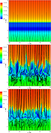Fig. 1. Spatial profiles of log(Ti) overlaid with magnetic field lines at t = 0 s (top) and t = 4000 s (middle and bottom), without electrons (middle) and with electrons (bottom).

The bottom plot corresponds to the scenario where electron collisions are taken into account. Here, the largest jet reaches y = 4 Mm and is located at x = 12 Mm. Furthermore, the maximum ion temperature values differ slightly: 1.5 × 10⁶ K in the case without electrons (this value agrees with the result obtained by Murawski et al. (2022)) and 1.4 × 10⁶ K with electrons.

Electron motion contributes to electric currents, which, in turn, influence the behavior of the magnetic field. Electrons are affected by the Lorentz force. This force can lead to the twisting and bending of magnetic field lines, contributing to changes in ||∇ × B||. Figure 2 presents spatial profiles of ||∇ × B|| for the cases without electrons (left) and with electrons (right). For the electrons dynamics that are ignored, the maximum value of ||∇ × B|| reaches about 7900 Gs Mm⁻¹, and is greater than in the case in which the electrons are taken into consideration, where max(||∇ × B||) ≈2600 Gs Mm⁻¹. Since ||∇ × B|| is nonzero, according to Eq. (10), the electrons attain different speeds than the ions, allowing them to exchange and thermalize their energies during collisions.

Fig. 2. Spatial profiles of ||∇ × B|| at t = 4000 s, for the models without electrons (left) and with electrons (right).

Figure 3 (top panels) presents time–distance plots for the horizontally averaged ion temperature, ⟨T_i⟩_x:

$$\begin{array}{c}\hfill {\langle T_{\mathrm{i}}\rangle }_x=\frac{1}{x_2-x_1}{\displaystyle {\int }_{x_1}^{x_2}}{T}_{\mathrm{i}}\mathrm{d}x,\end{array}$$(12)

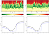Fig. 3. Time–distance plots for horizontally averaged ⟨Ti⟩x (top); the dashed line represents the semi-empirical model of Avrett & Loeser (2008) and averaged-over-time ion temperature ⟨Ti⟩xt (bottom), for the model without electrons (left) and with electrons (right).

where x₁ = −10.24 Mm and x₂ = 10.24 Mm. The only difference between the two plots is that the one on the left is based on a simulation in which collisions with electrons were ignored, while for the plots on the right, these collisions were included. It is clear that the plots are very similar, except that the values of the ion temperature are slightly higher in the case without electrons, max⟨T_i⟩_x = 2 × 10⁶ K; however, the difference is so small as to be negligible.

The same is true for the plots in the bottom panels, which show the horizontally and time-averaged ion temperature ⟨T_i⟩_xt, which can be defined as

$$\begin{array}{c}\hfill {\langle T_{\mathrm{i}}\rangle }_{x\mathrm{t}}=\frac{1}{t_2-t_1}{\displaystyle {\int }_{t_1}^{t_2}}{\langle T_{\mathrm{i}}\rangle }_x\mathrm{d}t,\end{array}$$(13)

where t₁ = 0 s and t₂ = 5000 s. In the case of the bottom-left panel, ⟨T_i⟩_xt reaches a maximum of only about 10⁶ K in the upper corona. The minimum value of about 10⁴ K occurs at the height of the bottom of the photosphere.

Additionally, we specify that

$$\begin{array}{c}\hfill \mathrm{\Delta }T\equiv {\langle \frac{T_{\mathrm{i}}-T}{T}\rangle }_{x\mathrm{t}y}=\frac{1}{y_2-y_1}{\displaystyle {\int }_{y_1}^{y_2}}\frac{{\langle T_{\mathrm{i}}\rangle }_{x\mathrm{t}}-T}{T}\mathrm{d}y,\end{array}$$(14)

where y₁ = 0 Mm, and y₂ = 2 Mm and T is the semi-empirical temperature (Avrett & Loeser 2008). When electron collisions were ignored, ΔT = 1.25; when electron collisions are taken into account, ΔT = 0.53. These results show that the presence of electrons does not significantly increase the amount of heat that is deposited in the atmosphere.

Figure 4 (top panels) shows time–distance plots for the relative perturbed ion temperature δT_i/T for simulations without (left) and with electrons (right). The top-left panel shows that max(δT_i/T) is about 300, whereas the top-right plot shows that the maximum value is about 350.

Fig. 4. Vertical profiles of relative perturbed ion temperature δTi/T (top) and averaged-over-time perturbed ion temperature (bottom) without electrons (left) and with electrons (right).

The bottom panels of Fig. 4 show the temporarily averaged perturbed temperature ⟨δT_i/T⟩_t. In the case of the bottom-left panel, ⟨δT_i/T⟩_t reaches a maximum of about 120 in the chromosphere (but higher up it rapidly decreases almost to 0 K). The bottom-right panel reveals a similar trend and shows that the maximum value occurs at the same height but is smaller – about 90. The observed difference in the height at which ion temperature perturbations begin can be attributed to the higher collision frequency at lower heights when electrons are included.

Figure 5 (top panels) presents time–distance plots for the vertical component of the horizontally averaged ion velocity ⟨V_iy⟩_x. The maximum value of the vertical component of the ion velocity in the case without electrons (left panel) is max(V_iy) ≈ 70 km s⁻¹, while with electrons, it is max(V_iy) ≈ 55 km s⁻¹.

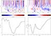Fig. 5. Time–distance plots for ⟨Viy⟩x (top) and time-averaged vertical ion velocity (bottom), without electrons (left) and with electrons (right).

The bottom panels of Fig. 5 show the time-averaged vertical ion velocity, which can be defined as

$$\begin{array}{c}\hfill {\langle V_{\mathrm{i}y}\rangle }_{\mathrm{t}x}=\frac{1}{t_2-t_1}{\displaystyle {\int }_{t_1}^{t_2}}{\langle V_{\mathrm{i}y}\rangle }_x\mathrm{d}t,\end{array}$$(15)

where t₁ = 0 s and t₂ = 5000 s. It is noticeable that in the case without electrons, downflows take place almost in the entire studied area up to y = 5 Mm, with the minimum velocity value of about 4.1 km s⁻¹ taking place at y ≈ 1 M. The panel on the right-hand side represents the case in which collisions with electrons were taken into account. Here, net downflows mainly take place, but they turn into upflows with a magnitude that increass with height y while moving from the lower atmosphere to the corona. Its minimum value reaches about 3.9 km s⁻¹ at y ≈ −1.2 M and the maximum value is approximately 0.9 km s⁻¹ at y ≈ 5 M.

Additionally, we specify that

$$\begin{array}{c}\hfill \mathrm{\Delta }V\equiv {\langle \frac{V_{\mathrm{i}y}}{c_{\mathrm{s}}}\rangle }_{\mathit{xty}}=\frac{1}{y_2-y_1}{\displaystyle {\int }_{y_1}^{y_2}}\frac{{\langle V_{\mathrm{i}y}\rangle }_{\mathit{xt}}}{c_{\mathrm{s}}}\mathrm{d}y,\end{array}$$(16)

where y₁ = 0 Mm, and y₂ = 2 Mm and c_s ≈ 10 km s⁻¹ is the local sound speed. For the case where electron collisions were not considered, ΔV = 0.2, and for the case with electrons, ΔV = 0.05. Equation (16) demonstrates that the Mach number of the generated upflows remains subsonic and does not vary significantly with or without the presence of electrons. This occurs because electrons lose energy through collisions in the lower part of the simulation domain, thereby reducing the energy available for conversion into the kinetic energy of the plasma upflows.

4. Summary and conclusion

Numerical simulations of chromosphere heating and plasma flows were performed in a partially ionized solar atmosphere, with nonadiabatic and nonideal effects taken into account and with electron effects included in the model. The considered model atmosphere was supplemented by spontaneously evolving and self-organizing convection, which excited waves and sheared plasma flows. The energy associated with these processes is dissipated by collisions, magnetic diffusivity, and viscosity, effectively heating the solar plasma and competing with radiative and thermal energy losses. This dissipation results in the local heating of the chromosphere.

Compared to the previous study by Murawski et al. (2022), who adopted a model without electron effects, our results show that electrons do not significantly affect the chromosphere heating and plasma outflows. The reason for their negligible effect lies in the physics of collisions and energy transfer within the solar atmosphere. Electrons are less effective in transferring energy through collisions due to their significantly lower mass compared to ions and neutrals. This reduces their ability to heat the plasma and generate significant flows. Conversely, ion–neutral collisions play a dominant role in these processes. They occur more frequently and involve larger energy exchanges, making them crucial for heating the plasma and driving atmospheric flows. Therefore, we conclude that while electrons are present and do contribute to energy transfer, their overall impact is negligible compared to ion–neutral collisions.

Acknowledgments

The original JOANNA code and the modules for the electrons were implemented by Dr. Darek Wójcik. This work was done within the framework of the projects from the Polish National Foundation (NCN) grant No. 2020/37/B/ST9/00184. Numerical simulations were performed on the MIRANDA cluster at Institute of Mathematics of University of M. Curie-Skłodowska, Lublin, Poland. We gratefully acknowledge Poland’s high-performance computing infrastructure PLGrid (HPC Centers: ACK Cyfronet AGH) for providing computer facilities and support within computational grant no. PLG/2022/015868. SP acknowledges support from the projects C14/19/089 (C1 project Internal Funds KU Leuven), G.0B58.23N and G.0025.23N (WEAVE) (FWO-Vlaanderen), 4000134474 (SIDC Data Exploitation, ESA Prodex-12), and Belspo project B2/191/P1/SWiM, as well as from SWATNet, a project that has received funding from the European Union’s Horizon 2020 research and innovation programme under the Marie Sklodowska-Curie grant agreement No 955620.

References

All Figures

	Fig. 1. Spatial profiles of log(Ti) overlaid with magnetic field lines at t = 0 s (top) and t = 4000 s (middle and bottom), without electrons (middle) and with electrons (bottom).
In the text

	Fig. 2. Spatial profiles of ||∇ × B|| at t = 4000 s, for the models without electrons (left) and with electrons (right).
In the text

	Fig. 3. Time–distance plots for horizontally averaged ⟨Ti⟩x (top); the dashed line represents the semi-empirical model of Avrett & Loeser (2008) and averaged-over-time ion temperature ⟨Ti⟩xt (bottom), for the model without electrons (left) and with electrons (right).
In the text

	Fig. 4. Vertical profiles of relative perturbed ion temperature δTi/T (top) and averaged-over-time perturbed ion temperature (bottom) without electrons (left) and with electrons (right).
In the text

	Fig. 5. Time–distance plots for ⟨Viy⟩x (top) and time-averaged vertical ion velocity (bottom), without electrons (left) and with electrons (right).
In the text

References

- Alharbi, A., Ballai, I., Fedun, V., & Verth, G. 2022, MNRAS, 511, 5274 [NASA ADS] [CrossRef] [Google Scholar]
- Aschwanden, M. J. 2005, Physics of the Solar Corona. An Introduction with Problems and Solutions, 2nd edn. (New York: Praxis Publishing Ltd) [Google Scholar]
- Avrett, E. H. 2003, ASP Conf. Ser., 286, 419 [NASA ADS] [Google Scholar]
- Avrett, E. H., & Loeser, R. 2008, ApJS, 175, 229 [Google Scholar]
- Braginskii, S. I. 1965, Rev. Plasma Phys., 1, 205 [Google Scholar]
- Brchnelova, M., Kuźma, B., Zhang, F., Lani, A., & Poedts, S. 2023, A&A, 678, A117 [NASA ADS] [CrossRef] [EDP Sciences] [Google Scholar]
- Dedner, A., Kemm, F., Kröner, D., et al. 2002, J. Comput. Phys., 175, 645 [Google Scholar]
- Durran, D. R. 2010, Numerical Methods for Fluid Dynamics (New York: Springer) [CrossRef] [Google Scholar]
- Khomenko, E., Collados, M., Díaz, A., & Vitas, N. 2014, Phys. Plasmas, 21, 092901 [Google Scholar]
- Kuźma, B., & Murawski, K. 2018, ApJ, 866, 50 [CrossRef] [Google Scholar]
- Meier, E. T., & Shumlak, U. 2012, Phys. Plasmas, 19, 072508 [NASA ADS] [CrossRef] [Google Scholar]
- Mignone, A., Bodo, G., & Ugliano, M. 2012, Numerical Methods for Hyperbolic Equations, 219 [Google Scholar]
- Miyoshi, T., & Kusano, K. 2007, AGU Fall Meeting Abstracts, 2007, SM41A-0311 [Google Scholar]
- Murawski, K., Musielak, Z. E., Poedts, S., Srivastava, A. K., & Kadowaki, L. 2022, Ap&SS, 367, 111 [NASA ADS] [CrossRef] [Google Scholar]
- Niedziela, R., Murawski, K., & Poedts, S. 2021, A&A, 652, A124 [NASA ADS] [CrossRef] [EDP Sciences] [Google Scholar]
- Niedziela, R., Murawski, K., Kadowaki, L., Zaqarashvili, T., & Poedts, S. 2022, A&A, 668, A32 [NASA ADS] [CrossRef] [EDP Sciences] [Google Scholar]
- Ofman, L. 2010, Liv. Rev. Sol. Phys., 7, 4 [Google Scholar]
- Pelekhata, M., Murawski, K., & Poedts, S. 2021, A&A, 652, A114 [NASA ADS] [CrossRef] [EDP Sciences] [Google Scholar]
- Pelekhata, M., Murawski, K., & Poedts, S. 2023, A&A, 669, A47 [NASA ADS] [CrossRef] [EDP Sciences] [Google Scholar]
- Toro, E. F., Hidalgo, A., & Dumbser, M. 2009, J. Comput. Phys., 228, 3368 [NASA ADS] [CrossRef] [Google Scholar]
- Uchida, Y., & Kaburaki, O. 1974, Sol. Phys., 35, 451 [NASA ADS] [CrossRef] [Google Scholar]
- Wójcik, D., Murawski, K., & Musielak, Z. E. 2018, MNRAS, 481, 262 [CrossRef] [Google Scholar]
- Wójcik, D., Kuźma, B., Murawski, K., & Srivastava, A. K. 2019, ApJ, 884, 127 [CrossRef] [Google Scholar]