© The Authors 2025

1. Introduction

It is well established that as a result of their low temperatures, neutrals dominate the photosphere, and the chromosphere is weakly ionized. The abundance of neutral atoms in these atmosphere layers leads to a modest two-fluid model in which ions combined with electrons and neutrals are described by magnetohydrodynamic (MHD) equations and hydrodynamic equations, respectively, and they are coupled by means of the collisional terms (e.g. Ballester et al. 2018). Based on these coupled equations, deviations from MHD were found both analytically (e.g. Kumar & Roberts 2003; Zaqarashvili et al. 2011; Soler et al. 2019) and numerically (e.g. Maneva et al. 2017; Kuźma et al. 2020). These non-MHD effects are important in the context of the heating of the chromosphere because the relative motions between ions and neutrals cause the collisional damping of Alfvén waves and the release of thermal energy (e.g. Vranjes et al. 2008).

One of the most outstanding issues of the solar atmosphere is the problem of energy transfer from the photosphere to the higher layers and the heating of the plasma. Alfvén waves are thought to play an important role in this transfer. They were described by Alfvén (1942) as waves that propagate along the magnetic lines and are driven by magnetic tension. An analytical approach to Alfvén waves in the two-fluid approximation can be found in Soler (2024), who presented the dispersion relation for linear Alfvén waves and confirmed that Alfvén waves are damped by neutral-ion collisions.

Recently, Kraśkiewicz et al. (2023) showed that driven two-fluid Alfvén waves exhibit the potential to heat the chromosphere. However, these studies were performed for magnetohydrostatic equilibrium with a straight vertical magnetic field. We study driven two-fluid Alfvén waves in a solar magnetic flux tube with diverging magnetic field lines with height and consider the magnetohydrostatic background supplemented by the Saha equation, which implies a realistic ionization profile in the solar atmosphere (Saha 1920).

The organization of the remainder of this paper is as follows. Sect. 2 describes the two-fluid equations, the background plasma models of the solar atmosphere, and the driven perturbations that were applied in the numerical simulations. Sect. 3 presents the results of the numerical simulations, and Sect. 4 contains a discussion and summary of the numerical results, together with the conclusions that we draw from them.

2. Numerical models of the solar atmosphere

The solar atmosphere is assumed to consist of hydrogen plasma, that is, of neutrals (hydrogen atoms) and ions (protons) + electrons, which are treated as two separate fluids. These fluids interact with each other through collisions described by ion-neutral drag force. The neutrals are governed by the following equations:

$$\begin{array}{cc}\hfill \frac{\partial {\varrho }_{\mathrm{n}}}{\partial t}+\mathrm{\nabla }·({\varrho }_{\mathrm{n}}{\mathbf{V}}_{\mathrm{n}})& ={\varrho }_{\mathrm{i}}{\mathrm{\Gamma }}_{\mathrm{n}}^{\mathrm{rec}}-{\varrho }_{\mathrm{n}}{\mathrm{\Gamma }}_{\mathrm{n}}^{\mathrm{ion}},\hfill \end{array}$$(1)

$$\begin{array}{cc}\hfill \frac{\partial ({\varrho }_{\mathrm{n}}{\mathbf{V}}_{\mathrm{n}})}{\partial t}+\mathrm{\nabla }·({\varrho }_{\mathrm{n}}{\mathbf{V}}_{\mathrm{n}}{\mathbf{V}}_{\mathrm{n}})& =-\mathrm{\nabla }{p}_{\mathrm{n}}+{\varrho }_{\mathrm{n}}\mathbf{g}-{\mathbf{S}}_{\mathrm{m}},\hfill \end{array}$$(2)

$$\begin{array}{cc}\hfill \frac{\partial E_{\mathrm{n}}}{\partial t}+\mathrm{\nabla }·[(E_{\mathrm{n}}+p_{\mathrm{n}}){\mathbf{V}}_{\mathrm{n}}]& =({\varrho }_{\mathrm{n}}\mathbf{g}-{\mathbf{S}}_{\mathrm{m}})·{\mathbf{V}}_{\mathrm{n}}+Q_{\mathrm{n}},\hfill \end{array}$$(3)

where the total energy density

$$\begin{array}{c}\hfill E_{\mathrm{n}}=\frac{{\varrho }_{\mathrm{n}}{\mathbf{V}}_{\mathrm{n}}^2}{2}+\frac{p_{\mathrm{n}}}{\gamma -1}·\end{array}$$(4)

The ions + electrons are described by

$$\begin{array}{cc}\hfill \frac{\partial {\varrho }_{\mathrm{i}}}{\partial t}+\mathrm{\nabla }·({\varrho }_{\mathrm{i}}{\mathbf{V}}_{\mathrm{i}})& ={\varrho }_{\mathrm{n}}{\mathrm{\Gamma }}_{\mathrm{n}}^{\mathrm{ion}}-{\varrho }_{\mathrm{i}}{\mathrm{\Gamma }}_{\mathrm{n}}^{\mathrm{rec}},\hfill \end{array}$$(5)

$$\begin{array}{cc}\hfill \frac{\partial ({\varrho }_{\mathrm{i}}{\mathbf{V}}_{\mathrm{i}})}{\partial t}+\mathrm{\nabla }·({\varrho }_{\mathrm{i}}{\mathbf{V}}_{\mathrm{i}}{\mathbf{V}}_{\mathrm{i}})& =\hfill \\ \hfill & -\mathrm{\nabla }(p_i+p_e)+\frac{1}{\mu }(\mathrm{\nabla }\times \mathbf{B})\times \mathbf{B}+{\varrho }_{\mathrm{i}}\mathbf{g}+{\mathbf{S}}_{\mathrm{m}},\hfill \end{array}$$(6)

$$\begin{array}{cc}\hfill \frac{\partial \mathbf{B}}{\partial t}& =\mathrm{\nabla }\times ({\mathbf{V}}_{\mathrm{i}}\times \mathbf{B})\text{with}\mathrm{\nabla }·\mathbf{B}=0,\hfill \end{array}$$(7)

$$\begin{array}{cc}\hfill \frac{\partial E_{\mathrm{i}}}{\partial t}+& \mathrm{\nabla }·[(E_{\mathrm{i}}+p_{\mathrm{i}}+p_{\mathrm{e}}+\frac{{\mathbf{B}}^2}{2\mu }){\mathbf{V}}_{\mathrm{i}}-\frac{\mathbf{B}}{\mu }({\mathbf{V}}_{\mathrm{i}}·\mathbf{B})]\hfill \\ \hfill & =({\varrho }_{\mathrm{i}}\mathbf{g}+{\mathbf{S}}_{\mathrm{m}})·{\mathbf{V}}_{\mathrm{i}}+Q_{\mathrm{i}},\hfill \end{array}$$(8)

where

$$\begin{array}{c}\hfill E_{\mathrm{i}}=\frac{{\varrho }_{\mathrm{n}}{\mathbf{V}}_{\mathrm{i}}^2}{2}+\frac{{\mathbf{B}}^2}{2\mu }+\frac{p_{\mathrm{i}}+p_{\mathrm{e}}}{\gamma -1}·\end{array}$$(9)

In Eqs. (1)–(9), the subscripts _i, _e, and _n correspond to ions, electrons, and neutrals, respectively. The symbols 𝜚_i, n denote the mass densities, V_i, n = [V_i, n x, V_i, n y, V_i, n z] are the velocities, p_e = p_i and p_n the gas pressures, B = [B_x, B_y, B_z] is the magnetic field, and T_i, n are the temperatures, specified by the ideal gas laws,

$$\begin{array}{c}\hfill p_{\mathrm{i},\mathrm{n}}=\frac{k_{\mathrm{B}}}{m_{\mathrm{i},\mathrm{n}}}{\varrho }_{\mathrm{i},\mathrm{n}}{T}_{\mathrm{i},\mathrm{n}},\end{array}$$(10)

with m_n ≃ m_i = m_H being the masses, and m_H is the hydrogen (proton) mass. Here, ${\mathrm{\Gamma }}_{\mathrm{i}}^{\mathrm{ion}}$ and ${\mathrm{\Gamma }}_{\mathrm{n}}^{\mathrm{rec}}$ are coefficients of ionization and recombination (Murawski et al. 2022) and the collisional momentum, S_m, and energy, Q_i, n, source terms are given as (Draine 1986)

$$\begin{array}{cc}\hfill {\mathbf{S}}_{\mathrm{m}}& ={\alpha }_{\mathrm{in}}({\mathbf{V}}_{\mathrm{n}}-{\mathbf{V}}_{\mathrm{i}})+{\mathrm{\Gamma }}_{\mathrm{i}}^{\mathrm{ion}}{\mathbf{S}}_{\mathrm{n}}-{\mathrm{\Gamma }}_{\mathrm{n}}^{\mathrm{rec}}{\mathbf{V}}_{\mathrm{i}},\hfill \\ \hfill Q_{\mathrm{n}}& =Q_{\mathrm{V}}+Q_{\mathrm{T}}+\frac{1}{2}({\varrho }_{\mathrm{i}}{\mathrm{\Gamma }}_{\mathrm{n}}^{\mathrm{rec}}{V}_{\mathrm{i}}^2-{\varrho }_{\mathrm{n}}{\mathrm{\Gamma }}_{\mathrm{n}}^{\mathrm{ion}}{V}_{\mathrm{n}}^2),\hfill \\ \hfill Q_{\mathrm{i}}& =Q_{\mathrm{V}}-Q_{\mathrm{T}}+\frac{1}{2}({\varrho }_{\mathrm{i}}{\mathrm{\Gamma }}_{\mathrm{i}}^{\mathrm{ion}}{V}_{\mathrm{n}}^2-{\varrho }_{\mathrm{n}}{\mathrm{\Gamma }}_{\mathrm{i}}^{\mathrm{rec}}{V}_{\mathrm{i}}^2),\hfill \end{array}$$(11)

with collisional heating,

$$\begin{array}{c}\hfill Q_{\mathrm{V}}=\frac{1}{2}{\alpha }_{\mathrm{in}}{(V_{\mathrm{i}}-V_{\mathrm{n}})}^2,\end{array}$$(12)

and thermal energy exchange,

$$\begin{array}{c}\hfill Q_{\mathrm{T}}=\frac{1}{\gamma -1}\frac{k_{\mathrm{B}}}{m_{\mathrm{n}}+m_{\mathrm{i}}}{\alpha }_{\mathrm{in}}(T_{\mathrm{i}}-T_{\mathrm{n}}),\end{array}$$(13)

terms. The gravitational acceleration vector g = [0, −g, 0] has a magnitude g = 274.78 m s⁻² on the Sun. The symbol k_B denotes the Boltzmann constant, γ = 5/3 is the ratio of specific heats, and μ means the magnetic permeability of the medium.

The coefficient of collisions between ions and neutrals is given by (Oliver et al. 2016)

$$\begin{array}{c}\hfill {\alpha }_{\mathrm{in}}=\frac{4}{3}\frac{{\sigma }_{\mathrm{in}}{\varrho }_{\mathrm{i}}{\varrho }_{\mathrm{n}}}{m_{\mathrm{i}}+m_{\mathrm{n}}}\sqrt{\frac{8k_{\mathrm{B}}}{\pi }(\frac{T_{\mathrm{i}}}{m_{\mathrm{i}}}+\frac{T_{\mathrm{n}}}{m_{\mathrm{n}}})},\end{array}$$(14)

where σ_in is the collisional cross-section, here taken as 1.4 × 10⁻¹⁹ m² (Vranjes & Krstic 2013). The Cartesian coordinate system was used with the x-axis horizontal, the y-axis vertical, and the z-axis lying along the ignorable direction with ∂/∂_z = 0, and V_i, nz and B_z being non-identically zero. In this system, the equilibrium quantities depend on x and y. The other symbols have their standard meaning (Murawski et al. 2022).

2.1. Static background

The solar atmosphere is a highly dynamical medium (e.g. Wedemeyer et al. 2004). However, we assumed that the solar atmosphere is initially in a static state, that is, all quantities are invariant of time, ∂/∂t = 0, and the atmosphere is still, V_i = V_n = 0.

The hydrostatic background was supplemented by the Saha equation (Saha 1920), from which realistic vertical profiles were obtained (Niedziela et al. 2024).

The background temperature, specified here by the semi-empirical model of Avrett & Loeser (2008), is shown in Fig. 1 (top). At the bottom of the photosphere, the top boundary of which is located at y = 0.5 Mm, T(y = 0)≈5800 K. Higher up, the temperature declines with height (y) in the photosphere and reaches its minimum of 4341 K in the low chromosphere, at y ≈ 0.6 Mm. Then, T grows with y to about 10⁶ K at y = 30 Mm in the corona, which occupies the region above the transition region, located at y = 2.1 Mm.

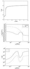Fig. 1. Top: Background temperature. Middle: 𝜚n (dashed line) and 𝜚i (solid line). Bottom: Neutral-ion τni (solid line) and ion-neutral τin (dashed line) collision times vs. height y.

The background ion (solid line) and neutral (dashed line) mass densities are displayed in Fig. 1 (middle). 𝜚_n is much larger than 𝜚_i in the photosphere and in the low chromosphere. In the corona, the opposite relation takes place. Mainly, 𝜚_n is much smaller than 𝜚_i there.

Figure 1 (bottom) displays the neutral-ion collision time, τ_ni = 𝜚_n/α_in, (solid line), and the ion-neutral collision time, τ_in = 𝜚_i/α_in, (dashed line) versus height. In the photosphere, 10⁻³ s ≲ τ_ni ≲ 10⁻¹ s. The local maximum of τ_ni is about 0.2 s and takes place in the low chromosphere at y ≈ 0.6 Mm, where T(y) attains its minimum. The local minimum of about 2 ⋅ 10⁻³ s can be found at y ≈ 1 Mm and τ_ni > 0.1 s in the low corona. In addition, τ_in is much smaller than τ_ni, which means that ion-neutral collisions are more frequent than neutral-ion collisions.

2.2. Flux-tube model

The hydrostatic background is overlaid by a current- and thus force-free magnetic field in the form of a magnetic arcade, given as

$$\begin{array}{cc}\hfill \mathbf{B}& =[B_{\mathrm{x}},B_{\mathrm{y}},0]=\hfill \\ \hfill & B_{0}exp\left(\frac{-y}{{\mathrm{\Lambda }}_{\mathrm{B}}}\right)[cos\left(\frac{x}{{\mathrm{\Lambda }}_{\mathrm{B}}}\right),-sin\left(\frac{x}{{\mathrm{\Lambda }}_{\mathrm{B}}}\right),0]+[0,B_{\mathrm{v}},0],\hfill \end{array}$$(15)

where B₀ is the flux-tube magnetic field at y = 0 Mm, B_v is the vertical magnetic field, chosen here to be equal to −10 G (unless otherwise stated), Λ_B = 2L/π is the magnetic scale height, with L being the arcade half-width, taken here as 1.28 Mm. The magnetic field lines, which diverge with height, are shown in Fig. 2 (top). The corresponding total Alfvén speed, $c_{\mathrm{A}}(x,y)=B/\sqrt{\mu ({\varrho }_{\mathrm{i}}+{\varrho }_{\mathrm{n}})}$, is illustrated in a color map. c_A achieves values of about 2 km s⁻¹ in the low photosphere. Higher up, it grows with y and takes the following values: c_A(x = 0, y = 2 Mm)≈500 km s⁻¹ up to its maximum value of about 2300 km s⁻¹ at y = 2.4 Mm. In the higher corona, c_A decreases to about 700 km s⁻¹ at y ≈ 6 Mm (Fig. 2, top).

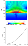Fig. 2. Initial (at t = 0 s) magnetic field lines overlaid with the Alfvén speed cA(x, y) in km s−1, (color map) (top) and cA(x = 0, y) (bottom).

2.3. Monochromatic driver

The magnetohydrostatic background described above is perturbed by a monochromatic driver specified in the transversal (z) components of the ion and neutral velocities as

$$\begin{array}{c}\hfill V_{\mathrm{iz}}(x,y=y_0,t)=V_{\mathit{nz}}(x,y=y_0,t)=V_{0}exp\left(\frac{-x^2}{w^2}\right)sin\left(\frac{2\pi }{P_{\mathrm{d}}}t\right).\end{array}$$(16)

Here, y₀ is the operation height, V₀ is the amplitude of the driver, w = 100 km denotes its width, and P_d stands for its period.

3. Numerical results

In this section, we present the results for 2.5 D numerical simulations performed using the code JOANNA (Wójcik et al. 2020). In the developed model, all plasma quantities were assumed to be invariant of z (∂/∂z = 0), but the transversal components of ion (V_iz) and neutral (V_nz) velocities and the magnetic field (B_z) were not identically zero. Prior to considering the flux-tube model, we show the numerical results for two simplified atmosphere models. In the first model, presented in Sect. 3.1, the solar gravity was set to 0 and all background quantities were assumed to be independent of x and y. This model serves for comparison purposes with the linear wave theory, and thus, for testing the code. In the second model, discussed in Sect. 3.2, the gravity was switched on, but the physical system was assumed to be invariant of x (∂/∂x = 0). In these two models, B₀ = 0 G and B_v = 10 G were set in Eq. (15). Finally, the flux-tube model was considered with B₀ = 500 G and B_v = −10 G (see Sect. 3.3).

3.1. A test for the gravity-free and homogeneous medium

We considered a gravity-free (g = 0) medium with constant values of the background quantities, mainly 𝜚_i = 10⁻⁹ kg m³, 𝜚_n = 10⁻⁸ kg m³, and T = 6676 K, and the magnetic field was taken to be vertical with B₀ = 0 and B_v = 10 G in Eq. (15). These values correspond to conditions in the upper chromosphere or low corona. For these conditions, τ_ni ≈ 10⁻² s. The two-fluid equations were solved numerically within the regions that are covered by the grid of 1024 cells with their vertical size, Δy, depending on P_d and varying from Δy = 0.01 km for P_d = 0.01 s to Δy = 0.1 km for P_d = 0.1 s. The simulation region also depends on P_d and was larger for larger P_d, and it varied from 10 km to 100 km.

Figure 3 displays the time-distance plot for V_iz for the driver, which is given by Eq. (16) with y₀ = 1 Mm, V₀ = 1 km s⁻¹, and P_d = 0.02 s. this is approximately ten times longer than neutral-ion collision time, τ_ni(y = 1 Mm), (Fig. 1, bottom). The Alfvén waves are damped while they propagate up from the driver.

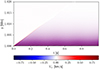Fig. 3. Time-distance plots for Viz(y, t) for the driver with Pd = 0.02 s in Eq. (16) operating in a gravity-free and homogeneous medium that mimics the chromosphere with a vertical magnetic field of Bv = 10 G.

To estimate the damping length of Alfvén waves, we adopted the following dispersion relation (Zaqarashvili et al. 2011):

$$\begin{array}{c}\hfill {\omega }^3+\mathrm{i}(1+\frac{{\varrho }_{\mathrm{n}}}{{\varrho }_{\mathrm{i}}}){\nu }_{\mathrm{ni}}{\omega }^2-k^2{c}_{\mathrm{A}}^2\omega -\mathrm{i}{\nu }_{\mathrm{ni}}{k}^2{c}_{\mathrm{A}}^2=0.\end{array}$$(17)

Here, ω = 2π/P_d and ν_ni = α_in/𝜚_n, are cyclic and neutral-ion collision frequencies, respectively, i² = −1, and k = k_r + ik_i denotes the complex wave number from which the wavelength is λ = 2π/k_r, and the damping length is λ_d = 2π/k_i.

Fig. 4 illustrates λ_d versus P_d obtained from the dispersion relation of Eq. (17) (solid line) and numerically by solving the two-fluid equations (dashed line). We infer that λ_d grows with P_d, meaning that waves with longer periods experience less attenuation than waves with shorter periods, and the trend is non-linear. For P_d = 0.01 s, the Alfvén waves are strongly damped with λ_d = 5 km. For P_d = 0.1 s, the Alfvén waves are less strongly damped with λ_d = 500 km. The numerical and analytical values of λ_d converge and reach similar values for all the selected values of P_d.

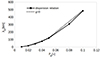Fig. 4. Damping length, λd, obtained from the dispersion relation of Eq. (17) (solid line) and numerically (dashed line) for the driver with V0 = 1 km s−1 operating at y0 = 1 Mm in a gravity-free homogeneous background.

3.2. The gravitationally stratified solar atmosphere model with a vertical magnetic field

In this part of the paper, we present the numerical results for the gravitationally stratified solar atmosphere model, with x being the invariant coordinate (∂/∂x = 0). In Eq. (15), B₀ was set to 0 G and B_v = 10 G. The numerical simulations were performed in the region y₀ ≤ y ≤ y₀ + 2.56 Mm with the grid resolution Δy = 0.625 km. Several values of y₀ were considered, such as y₀ = 0.6 Mm, y₀ = 0.8 Mm, and y₀ = 1 Mm. The driver operates at y = y₀ with an amplitude V₀ = 1 km s⁻¹ and a period P_d = 2.5 s.

Figure 5 illustrates time-distance plots for V_iz and y₀ = 0.8 Mm. The Alfvén waves are clearly damped. Parametric studies made for various values of y₀ revealed that the damping length, λ_d, decreases with y₀ < 0.8 Mm, and it grows higher up with y₀ (Fig. 6, dots). This behavior may result from the specific dependence of the ion and neutral mass densities on the height in the vicinity of y = 0.8 Mm (Fig. 1, middle). In particular, for y₀ = 0.6 Mm and y₀ = 1.0 Mm, the values of λ_d are 40 km and 100 km, respectively, which is close to the range of values of λ_d derived for the homogeneous atmosphere model (Fig. 4), which were obtained for P_d ≤ 0.05 s. However, for P_d = 2.5 s from the dispersion relation of Eq. (17) and for 𝜚_i, 𝜚_n, and T corresponding to y₀ = 0.8 Mm, we obtain that λ_d ≈ 7 km, which is lower by more than three times than the numerical value of λ_d ≈ 25 km. At the other heights, the difference between λ_d, calculated numerically and from the dispersion relation, is also significant (Fig. 6). The dispersion relation is strictly valid for a homogeneous medium, and therefore, it is a crude description for the low chromosphere, which is a strongly stratified medium. Therefore, the dispersion relation was only used here for reference purposes and should be taken with caution. As the numerical values of λ_d are lower than 100 km for y₀ < 1 Mm, we infer that Alfvén waves deposit their kinetic energy in the form of thermal energy in the chromosphere, and for higher values of y₀, the Alfvén waves experience weaker damping (Fig. 6).

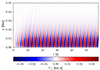Fig. 5. Time-distance plots for Viz(y, t) for the driver located at y0 = y0 = 0.8 Mm with Pd = 2.5 s in Eq. (16) for a solar chromosphere with ∂/∂x = 0, g ≠ 0, and a vertical magnetic field Bv = 10 G.

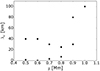Fig. 6. Damping length of Alfvén waves vs. the position of the driver with Pd = 2.5 s and V0 = 1 km s−1 in Eq. (16) (dots) for the solar chromosphere with Bv = 10 G and obtained from the dispersion relation of Eq. (17) (asterisks).

The values of y₀ listed above are close to the height at which the neutral-ion collision time reaches its local extrema: the maximum at y ≈ 0.6 Mm and the minimum at y ≈ 1 Mm (Fig. 1, bottom, solid line). The presence of this maximum results in strong damping of Alfvén waves, which was much weaker in the case of the hydrostatic equilibrium recently studied by Kraśkiewicz et al. (2023).

3.3. The solar atmosphere with a flux tube

In this part of the paper, we present the numerical results for the solar atmosphere with a flux tube. For the flux tube, a fine grid, which was used in the cases of the vertical magnetic field, would lead to too costly numerical simulations. Therefore, a uniform grid with its vertical size Δy = 2.5 km was set (except for P_d = 2.5 s where Δy = 1 km), which extends over the region 0 ≤ y ≤ 2.56 Mm. For higher values of y, the computational box was covered by 64 grid points up to y = 20 Mm. Along the x-direction, which is given as |x|≤2.56 Mm, the size of a numerical cell was set to Δx = 5 km. The monochromatic driver operates at the bottom of the photosphere, given by y₀ = 0 Mm, with its amplitude V₀ = 1 km s⁻¹ in Eq. (16).

Figure 7 (top) displays time-distance plots for V_iz(x = 0, y, t) for the driver with P_d = 2.5 s (left) and P_d = 10 s (right). For P_d = 2.5 s, the Alfvén waves are attenuated with significant amplitude that decreases with height. For P_d = 10 s, the amplitude of the Alfvén waves decreases weakly with height for y < 0.2 Mm. However, higher up, their amplitude starts to grow, and in effect, the waves reach the transition region and the corona.

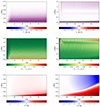Fig. 7. Time-distance plots for Viz(x = 0, y, t) (top), |Viz − Vnz| (middle), and δTi (bottom) for a solar atmosphere with a flux tube for the driver with Pd = 2.5 s (left) and Pd = 10 s (right).

As the transverse velocity drift, ΔV_z ≡ |V_iz − V_nz|, reaches finite numbers (Fig. 7, middle), it results in plasma heating by Alfvén waves. For P_d = 2.5 s, a magnitude of ΔV_z reaches its maximum of about 0.4 m s⁻¹ above y = 0 Mm, and higher up, it decreases along with the attenuation of the Alfvén waves. For P_d = 10 s, max(ΔV_z) ≈ 1.5 m s⁻¹ and it takes place at y ≈ 0.7 Mm which is at a higher altitude than in the case of P_d = 2.5 s.

As a result of ΔV_z > 0, the Alfvén waves thermalize their kinetic energy and warm the atmosphere while they are damped by ion-neutral collisions. Fig. 7 (bottom) illustrates the relative perturbed ion temperature, defined as δT_i = 100% (T_i − T)/T. Here, T(y) is the temperature at t = 0 (Fig. 1, top). For P_d = 2.5 s and P_d = 10 s, δT_i reaches a value of about 4% at y ≈ 0.01 Mm and y ≈ 0.04 Mm, respectively. Hence, we infer that for P_d = 2.5 s, Alfvén waves result in plasma heating at a lower height than for P_d = 10 s.

Figure 8 shows how the numerically estimated damping length, λ_d, depends on P_d. For P_d = 2.5 s, λ_d ≈ 50 km, and for higher values of P_d, λ_d grows, achieving for P_d = 5 s and P_d = 10 s values of λ_d ≈ 70 km and λ_d ≈ 200 km, respectively. Even though these values of λ_d correspond to a damping of Alfvén waves in the photosphere, they have similar magnitudes as λ_d evaluated in the chromosphere (compare the values of λ_d in Figs. 4, 6, and 8).

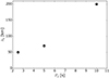Fig. 8. Damping length λd vs. Pd obtained numerically for Alfvén waves propagating along the flux tube.

4. Summary and conclusions

We constructed a model of a solar magnetic flux tube with a background state that was governed by the magnetohydrostatic conditions supplemented by the Saha equation. This model is an extension of the model discussed by Kraśkiewicz et al. (2023), who studied driven Alfvén waves in a purely hydrostatic atmosphere with a vertical magnetic field. In both models, the solar atmosphere was described by two-fluid equations for ions (protons) + electrons and neutrals (hydrogen atoms), which were treated as two separate fluids. However, in the model we developed, a realistic ionization profile and ionization and recombination were additionally implied. These equations were solved numerically with the use of the code JOANNA (Wójcik et al. 2020). Two-fluid Alfvén waves were excited in this atmosphere by a monochromatic driver. To test the code and for comparison purposes, two simplified models of the solar atmosphere were constructed that either corresponded to a gravity-free and homogeneous chromosphere or to a gravitationally stratified but horizontally invariant atmosphere. A straight vertical magnetic field was implemented in both models. The test for the gravity-free atmosphere model revealed that the values of the numerically estimated damping length of Alfvén waves were close to the analytical data that were obtained from the dispersion relation.

From the numerical results for the model of the solar atmosphere, which is gravitationally stratified, we inferred that Alfvén waves experience damping by ion-neutral collisions, with stronger effects corresponding to waves with shorter periods, and this damping is stronger than in the purely hydrostatic case considered by Kraśkiewicz et al. (2023). As a result, we claim that the presence of the realistic ionization profile and ionization and recombination plays an important role in Alfvén waves damping and thus in the thermalization of their energy, which contributes to the heating of the solar atomosphere.

Acknowledgments

The authors express their thanks to Dr. Fan Zhang for a few discussions during the initial phase of this project evolution. KM’s work was done within the framework of the project from the Polish Science Center (NCN) Grant No. 2020/37/B/ST9/00184. The Saha equation-based hydrostatic background was implemented into the code JOANNA by Dr. Luis Kadowaki during his research funded by the grant. All numerical simulations was run on the LUNAR cluster at the Institute of Mathematics at M. Curie-Sklodowska University in Lublin, Poland. The simulation data was visualized using the ViSIt software package (Childs et al. 2012) and Python scripts.

References

All Figures

	Fig. 1. Top: Background temperature. Middle: 𝜚n (dashed line) and 𝜚i (solid line). Bottom: Neutral-ion τni (solid line) and ion-neutral τin (dashed line) collision times vs. height y.
In the text

	Fig. 2. Initial (at t = 0 s) magnetic field lines overlaid with the Alfvén speed cA(x, y) in km s−1, (color map) (top) and cA(x = 0, y) (bottom).
In the text

	Fig. 3. Time-distance plots for Viz(y, t) for the driver with Pd = 0.02 s in Eq. (16) operating in a gravity-free and homogeneous medium that mimics the chromosphere with a vertical magnetic field of Bv = 10 G.
In the text

	Fig. 4. Damping length, λd, obtained from the dispersion relation of Eq. (17) (solid line) and numerically (dashed line) for the driver with V0 = 1 km s−1 operating at y0 = 1 Mm in a gravity-free homogeneous background.
In the text

	Fig. 5. Time-distance plots for Viz(y, t) for the driver located at y0 = y0 = 0.8 Mm with Pd = 2.5 s in Eq. (16) for a solar chromosphere with ∂/∂x = 0, g ≠ 0, and a vertical magnetic field Bv = 10 G.
In the text

	Fig. 6. Damping length of Alfvén waves vs. the position of the driver with Pd = 2.5 s and V0 = 1 km s−1 in Eq. (16) (dots) for the solar chromosphere with Bv = 10 G and obtained from the dispersion relation of Eq. (17) (asterisks).
In the text

	Fig. 7. Time-distance plots for Viz(x = 0, y, t) (top), |Viz − Vnz| (middle), and δTi (bottom) for a solar atmosphere with a flux tube for the driver with Pd = 2.5 s (left) and Pd = 10 s (right).
In the text

	Fig. 8. Damping length λd vs. Pd obtained numerically for Alfvén waves propagating along the flux tube.
In the text

References

- Alfvén, H. 1942, Nature, 150, 405 [Google Scholar]
- Avrett, E. H., & Loeser, R. 2008, ApJS, 175, 229 [Google Scholar]
- Ballester, J. L., Alexeev, I., Collados, M., et al. 2018, Space Sci. Rev., 214, 58 [Google Scholar]
- Childs, H., Brugger, E., Whitlock, B., et al. 2012, VisIt: An End-User Tool For Visualizing and Analyzing Very Large Data (Chapman and Hall/CRC), 357 [Google Scholar]
- Draine, B. T. 1986, MNRAS, 220, 133 [NASA ADS] [Google Scholar]
- Kraśkiewicz, J., Murawski, K., Zhang, F., & Poedts, S. 2023, Sol. Phys., 298, 11 [CrossRef] [Google Scholar]
- Kumar, N., & Roberts, B. 2003, Sol. Phys., 214, 241 [Google Scholar]
- Kuźma, B., Wójcik, D., Murawski, K., Yuan, D., & Poedts, S. 2020, A&A, 639, A45 [NASA ADS] [CrossRef] [EDP Sciences] [Google Scholar]
- Maneva, Y. G., Alvarez Laguna, A., Lani, A., & Poedts, S. 2017, ApJ, 836, 197 [Google Scholar]
- Murawski, K., Musielak, Z. E., Poedts, S., Srivastava, A. K., & Kadowaki, L. 2022, Ap&SS, 367, 111 [NASA ADS] [CrossRef] [Google Scholar]
- Niedziela, R., Murawski, K., & Poedts, S. 2024, A&A, 691, A254 [NASA ADS] [CrossRef] [EDP Sciences] [Google Scholar]
- Oliver, R., Soler, R., Terradas, J., & Zaqarashvili, T. V. 2016, ApJ, 818, 128 [Google Scholar]
- Saha, M. N. 1920, Nature, 105, 232 [CrossRef] [Google Scholar]
- Soler, R. 2024, Philos. Trans. R. Soc. Lond. Ser. A, 382, 20230223 [Google Scholar]
- Soler, R., Terradas, J., Oliver, R., & Ballester, J. L. 2019, ApJ, 871, 3 [Google Scholar]
- Vranjes, J., & Krstic, P. S. 2013, A&A, 554, A22 [NASA ADS] [CrossRef] [EDP Sciences] [Google Scholar]
- Vranjes, J., Poedts, S., Pandey, B. P., & De Pontieu, B. 2008, A&A, 478, 553 [NASA ADS] [CrossRef] [EDP Sciences] [Google Scholar]
- Wedemeyer, S., Freytag, B., Steffen, M., Ludwig, H.-G., & Holweger, H. 2004, A&A, 414, 1121 [NASA ADS] [CrossRef] [EDP Sciences] [Google Scholar]
- Wójcik, D., Kuźma, B., Murawski, K., & Musielak, Z. E. 2020, A&A, 635, A28 [NASA ADS] [CrossRef] [EDP Sciences] [Google Scholar]
- Zaqarashvili, T. V., Khodachenko, M. L., & Rucker, H. O. 2011, A&A, 534, A93 [NASA ADS] [CrossRef] [EDP Sciences] [Google Scholar]